Demo: Landsat background and data download#
UW Geospatial Data Analysis
CEE467/CEWA567
David Shean, Eric Gagliano, Quinn Brencher
Introduction#
In this demo, we’re going to download the Landsat 8 data that we’ll need for this module. While the data is being downloaded, we’ll briefly go over the Landsat program and the Landsat 8 data we’ll be working with.
The Landsat 8 mission#
The joint NASA and USGS Landsat program has been acquiring multi-spectral satellite imagery since 1972.
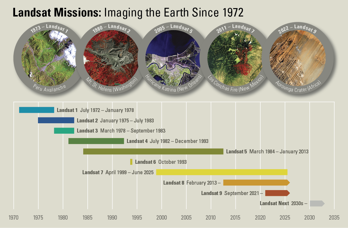
Timeline of the Landsat program, beginning with the launch of Landsat 1 in 1972. Landsat Next, consisting of a trio of satellite observatories, is expected to launch in late 2030. As the tenth Landsat mission, it will continue the legacy of the Landsat program.
Orbit and data collection#
Landsat 8 orbits the the Earth in a sun-synchronous, near-polar orbit, at an altitude of 705 km (438 mi), inclined at 98.2 degrees, and completes one Earth orbit every 99 minutes. The satellite has a 16-day repeat cycle with an equatorial crossing time: 10:00 a.m. +/- 15 minutes.
Landsat 8 aquires about 740 scenes a day on the Worldwide Reference System-2 (WRS-2) path/row system, with a swath overlap (or sidelap) varying from 7 percent at the equator to a maximum of approximately 85 percent at extreme latitudes. A Landsat 8 scene size is 185 km x 180 km (114 mi x 112 mi).
Instruments and bands#
Landsat-8 has two instruments…
Operational Land Imager (OLI)
Thermal Infrared Sensor (TIRS)
 The OLI collects data for two new bands, a coastal/aerosol band (band 1) and a cirrus band (band 9), as well as the heritage Landsat multispectral bands. Additionally, the bandwidth has been refined for six of the heritage bands. The Thermal Instrument (TIRS) carries two additional thermal infrared bands. Note: atmospheric transmission values for this graphic were calculated using MODTRAN for a summertime mid-latitude hazy atmosphere (circa 5 km visibility). Graphic via USGS
Image resolution - Ground Sample Distance (GSD)#
Panchromatic (PAN) band (band number 8) has 15 m ground sample distance (GSD)
Multispectral (MS) bands are 30 m GSD
Thermal IR are 100 m GSD, but are often oversampled to match MS bands
Dynamic range#
LS8 OLI provides 12-bit dynamic range, which improves characterization and signal to noise ratio. 12 bits means 2^12 (or 4096) unique combinations to represent brightness in the image.
We don’t have a convenient mechanism to store 12-bit data, so the LS8 images are stored as 16-bit unsigned integers. The initial values (spanning 0-4095) are scaled across 55000 of the total 65535 brightness levels in the 16-bit images.
Data products#
The standard data products are “Level 1” images, which are radiometrically corrected and orthorectified (terrain corrected) in the approprate UTM projection
For more sophisticated analysis, you typically want to use the higher-level “Level 2”, calibrated/corrected surface reflectance products, often considered “Analysis Ready Data (ARD)”
You’ll often see Digital Number (DN), top of atmosphere (TOA) and surface reflectance (SR)
“Top-of-atmosphere reflectance (or TOA reflectance) is the reflectance measured by a space-based sensor flying higher than the earth’s atmosphere. These reflectance values will include contributions from clouds and atmospheric aerosols and gases.”
Formulas for conversion of DN to TOA
“Surface reflectance (SR) is the amount of light reflected by the surface of the Earth. It is a ratio of surface radiance to surface irradiance, and as such is unitless, with values between 0 and 1.”
“Surface reflectance improves comparison between multiple images over the same region by accounting for atmospheric effects such as aerosol scattering and thin clouds, which can help in the detection and characterization of Earth surface change. “
More information here.
Data availability#
USGS/NASA hosts the official Landsat products on EarthExplorer. This option is great for one-off interactive data searches, but can be clunky and requires a lot of manual steps
Commercial cloud providers now mirror the entire USGS archive, and provide a much more efficient API (application programming interface) to access the data. This is especially important when you need to access 100s-1000s of images.
Finding imagery#
The process of identifying and downloading data has evolved considerably throughout the Landsat missions, and modern approaches use on-demand access to cloud-hosted archives, often without local downloads. We will opt for a programmatic approach, using pystac/pystac-client to query a SpatioTemporal Asset Catalog (STAC)
Other approaches include…
Interactive, manual approach. EarthExplorer for visual queries, and either download directly, or save image ID and use another approach.
For now, we’ll use the following code to download some pre-identified images for WA state to the hub. Note that we could do all of this on the fly, but for experimentation and development, having a local copy of sample images will speed up reading.
Download#
import pystac
from pystac_client import Client
import planetary_computer
import odc.stac
import matplotlib.pyplot as plt
import os
from pathlib import Path
import urllib
import rioxarray
imgdir = f'{Path.home()}/gda_demo_data/LS8_data'

if not os.path.exists(imgdir):
    os.makedirs(imgdir)
#Collection and bands (specific bands for L2 surface reflectance/temperature products)
collection = 'landsat-c2-l2'
asset_id_list = ['SR_B1', 'SR_B2', 'SR_B3', 'SR_B4', 'SR_B5', 'SR_B6', 'ST_B10', 'reduced_resolution_browse']
asset_id_list = ['coastal', 'blue', 'green', 'red', 'nir08', 'swir16', 'lwir11', 'rendered_preview']

#Bounding box
bbox = [-121.9,46.7,-121.6,47.0]

#Date range
dt = '2018-08-17/2018-12-26'

catalog = Client.open("https://planetarycomputer.microsoft.com/api/stac/v1",modifier=planetary_computer.sign_inplace)

results = catalog.search(
    collections=[collection],
    bbox=bbox,
    datetime=dt,
    query={
        "eo:cloud_cover": {"lt": 50},
        "landsat:wrs_path": {"eq": "046"}, # Path 46, Row 27 is the tile that contains Seattle and Mt. Rainier!
        "landsat:wrs_row": {"eq": "027"},
    },
)

# Check how many items were returned
items = list(results.items())
print(f"Returned {len(items)} Items")
Returned 7 Items
# let's just take the first and last set of images so we get an image in august and an image from december...
items = [items[0],items[6]]
items
[<Item id=LC08_L2SP_046027_20181224_02_T1>,
 <Item id=LC08_L2SP_046027_20180818_02_T1>]
items[0]
- type "Feature"
- stac_version "1.1.0"
stac_extensions[] 7 items
- 0 "https://stac-extensions.github.io/raster/v1.1.0/schema.json"
- 1 "https://stac-extensions.github.io/eo/v1.1.0/schema.json"
- 2 "https://stac-extensions.github.io/view/v1.0.0/schema.json"
- 3 "https://stac-extensions.github.io/projection/v2.0.0/schema.json"
- 4 "https://landsat.usgs.gov/stac/landsat-extension/v1.1.1/schema.json"
- 5 "https://stac-extensions.github.io/classification/v2.0.0/schema.json"
- 6 "https://stac-extensions.github.io/scientific/v1.0.0/schema.json"
- id "LC08_L2SP_046027_20181224_02_T1"
geometry
- type "Polygon"
coordinates[] 1 items
0[] 5 items
0[] 2 items
- 0 -122.7072203
- 1 48.5074494
1[] 2 items
- 0 -120.274416
- 1 48.0771131
2[] 2 items
- 0 -120.9719817
- 1 46.376193
3[] 2 items
- 0 -123.3291268
- 1 46.8005687
4[] 2 items
- 0 -122.7072203
- 1 48.5074494
bbox[] 4 items
- 0 -123.36848493
- 1 46.35421508
- 2 -120.21354706
- 3 48.51236492
properties
- gsd 30
- created "2022-05-06T17:33:53.536804Z"
- sci:doi "10.5066/P9OGBGM6"
- datetime "2018-12-24T18:55:31.840624Z"
- platform "landsat-8"
proj:shape[] 2 items
- 0 7881
- 1 7771
- description "Landsat Collection 2 Level-2"
instruments[] 2 items
- 0 "oli"
- 1 "tirs"
- eo:cloud_cover 32.34
proj:transform[] 6 items
- 0 30.0
- 1 0.0
- 2 472785.0
- 3 0.0
- 4 -30.0
- 5 5373315.0
- view:off_nadir 0
- landsat:wrs_row "027"
- landsat:scene_id "LC80460272018358LGN00"
- landsat:wrs_path "046"
- landsat:wrs_type "2"
- view:sun_azimuth 162.85812866
- landsat:correction "L2SP"
- view:sun_elevation 17.34244461
- landsat:cloud_cover_land 33.38
- landsat:collection_number "02"
- landsat:collection_category "T1"
- proj:code "EPSG:32610"
links[] 8 items
0
- rel "collection"
- href "https://planetarycomputer.microsoft.com/api/stac/v1/collections/landsat-c2-l2"
- type "application/json"
1
- rel "parent"
- href "https://planetarycomputer.microsoft.com/api/stac/v1/collections/landsat-c2-l2"
- type "application/json"
2
- rel "root"
- href "https://planetarycomputer.microsoft.com/api/stac/v1"
- type "application/json"
- title "Microsoft Planetary Computer STAC API"
3
- rel "self"
- href "https://planetarycomputer.microsoft.com/api/stac/v1/collections/landsat-c2-l2/items/LC08_L2SP_046027_20181224_02_T1"
- type "application/geo+json"
4
- rel "cite-as"
- href "https://doi.org/10.5066/P9OGBGM6"
- title "Landsat 8-9 OLI/TIRS Collection 2 Level-2"
5
- rel "via"
- href "https://landsatlook.usgs.gov/stac-server/collections/landsat-c2l2-sr/items/LC08_L2SP_046027_20181224_20200829_02_T1_SR"
- type "application/json"
- title "USGS STAC Item"
6
- rel "via"
- href "https://landsatlook.usgs.gov/stac-server/collections/landsat-c2l2-st/items/LC08_L2SP_046027_20181224_20200829_02_T1_ST"
- type "application/json"
- title "USGS STAC Item"
7
- rel "preview"
- href "https://planetarycomputer.microsoft.com/api/data/v1/item/map?collection=landsat-c2-l2&item=LC08_L2SP_046027_20181224_02_T1"
- type "text/html"
- title "Map of item"
assets
qa
- href "https://landsateuwest.blob.core.windows.net/landsat-c2/level-2/standard/oli-tirs/2018/046/027/LC08_L2SP_046027_20181224_20200829_02_T1/LC08_L2SP_046027_20181224_20200829_02_T1_ST_QA.TIF?st=2026-01-25T22%3A17%3A34Z&se=2026-01-26T23%3A02%3A34Z&sp=rl&sv=2025-07-05&sr=c&skoid=9c8ff44a-6a2c-4dfb-b298-1c9212f64d9a&sktid=72f988bf-86f1-41af-91ab-2d7cd011db47&skt=2026-01-26T06%3A46%3A59Z&ske=2026-02-02T06%3A46%3A59Z&sks=b&skv=2025-07-05&sig=5DWlK65HZBjyTlT6xdtasG5EwDRZzeM%2Bw04gH%2Bspbz4%3D"
- type "image/tiff; application=geotiff; profile=cloud-optimized"
- title "Surface Temperature Quality Assessment Band"
- description "Collection 2 Level-2 Quality Assessment Band (ST_QA) Surface Temperature Product"
raster:bands[] 1 items
0
- unit "kelvin"
- scale 0.01
- nodata -9999
- data_type "int16"
- spatial_resolution 30
roles[] 1 items
- 0 "data"
ang
- href "https://landsateuwest.blob.core.windows.net/landsat-c2/level-2/standard/oli-tirs/2018/046/027/LC08_L2SP_046027_20181224_20200829_02_T1/LC08_L2SP_046027_20181224_20200829_02_T1_ANG.txt?st=2026-01-25T22%3A17%3A34Z&se=2026-01-26T23%3A02%3A34Z&sp=rl&sv=2025-07-05&sr=c&skoid=9c8ff44a-6a2c-4dfb-b298-1c9212f64d9a&sktid=72f988bf-86f1-41af-91ab-2d7cd011db47&skt=2026-01-26T06%3A46%3A59Z&ske=2026-02-02T06%3A46%3A59Z&sks=b&skv=2025-07-05&sig=5DWlK65HZBjyTlT6xdtasG5EwDRZzeM%2Bw04gH%2Bspbz4%3D"
- type "text/plain"
- title "Angle Coefficients File"
- description "Collection 2 Level-1 Angle Coefficients File"
roles[] 1 items
- 0 "metadata"
red
- href "https://landsateuwest.blob.core.windows.net/landsat-c2/level-2/standard/oli-tirs/2018/046/027/LC08_L2SP_046027_20181224_20200829_02_T1/LC08_L2SP_046027_20181224_20200829_02_T1_SR_B4.TIF?st=2026-01-25T22%3A17%3A34Z&se=2026-01-26T23%3A02%3A34Z&sp=rl&sv=2025-07-05&sr=c&skoid=9c8ff44a-6a2c-4dfb-b298-1c9212f64d9a&sktid=72f988bf-86f1-41af-91ab-2d7cd011db47&skt=2026-01-26T06%3A46%3A59Z&ske=2026-02-02T06%3A46%3A59Z&sks=b&skv=2025-07-05&sig=5DWlK65HZBjyTlT6xdtasG5EwDRZzeM%2Bw04gH%2Bspbz4%3D"
- type "image/tiff; application=geotiff; profile=cloud-optimized"
- title "Red Band"
- description "Collection 2 Level-2 Red Band (SR_B4) Surface Reflectance"
eo:bands[] 1 items
0
- name "OLI_B4"
- center_wavelength 0.65
- full_width_half_max 0.04
- common_name "red"
- description "Visible red"
raster:bands[] 1 items
0
- scale 2.75e-05
- nodata 0
- offset -0.2
- data_type "uint16"
- spatial_resolution 30
roles[] 2 items
- 0 "data"
- 1 "reflectance"
blue
- href "https://landsateuwest.blob.core.windows.net/landsat-c2/level-2/standard/oli-tirs/2018/046/027/LC08_L2SP_046027_20181224_20200829_02_T1/LC08_L2SP_046027_20181224_20200829_02_T1_SR_B2.TIF?st=2026-01-25T22%3A17%3A34Z&se=2026-01-26T23%3A02%3A34Z&sp=rl&sv=2025-07-05&sr=c&skoid=9c8ff44a-6a2c-4dfb-b298-1c9212f64d9a&sktid=72f988bf-86f1-41af-91ab-2d7cd011db47&skt=2026-01-26T06%3A46%3A59Z&ske=2026-02-02T06%3A46%3A59Z&sks=b&skv=2025-07-05&sig=5DWlK65HZBjyTlT6xdtasG5EwDRZzeM%2Bw04gH%2Bspbz4%3D"
- type "image/tiff; application=geotiff; profile=cloud-optimized"
- title "Blue Band"
- description "Collection 2 Level-2 Blue Band (SR_B2) Surface Reflectance"
eo:bands[] 1 items
0
- name "OLI_B2"
- center_wavelength 0.48
- full_width_half_max 0.06
- common_name "blue"
- description "Visible blue"
raster:bands[] 1 items
0
- scale 2.75e-05
- nodata 0
- offset -0.2
- data_type "uint16"
- spatial_resolution 30
roles[] 2 items
- 0 "data"
- 1 "reflectance"
drad
- href "https://landsateuwest.blob.core.windows.net/landsat-c2/level-2/standard/oli-tirs/2018/046/027/LC08_L2SP_046027_20181224_20200829_02_T1/LC08_L2SP_046027_20181224_20200829_02_T1_ST_DRAD.TIF?st=2026-01-25T22%3A17%3A34Z&se=2026-01-26T23%3A02%3A34Z&sp=rl&sv=2025-07-05&sr=c&skoid=9c8ff44a-6a2c-4dfb-b298-1c9212f64d9a&sktid=72f988bf-86f1-41af-91ab-2d7cd011db47&skt=2026-01-26T06%3A46%3A59Z&ske=2026-02-02T06%3A46%3A59Z&sks=b&skv=2025-07-05&sig=5DWlK65HZBjyTlT6xdtasG5EwDRZzeM%2Bw04gH%2Bspbz4%3D"
- type "image/tiff; application=geotiff; profile=cloud-optimized"
- title "Downwelled Radiance Band"
- description "Collection 2 Level-2 Downwelled Radiance Band (ST_DRAD) Surface Temperature Product"
raster:bands[] 1 items
0
- unit "watt/steradian/square_meter/micrometer"
- scale 0.001
- nodata -9999
- data_type "int16"
- spatial_resolution 30
roles[] 1 items
- 0 "data"
emis
- href "https://landsateuwest.blob.core.windows.net/landsat-c2/level-2/standard/oli-tirs/2018/046/027/LC08_L2SP_046027_20181224_20200829_02_T1/LC08_L2SP_046027_20181224_20200829_02_T1_ST_EMIS.TIF?st=2026-01-25T22%3A17%3A34Z&se=2026-01-26T23%3A02%3A34Z&sp=rl&sv=2025-07-05&sr=c&skoid=9c8ff44a-6a2c-4dfb-b298-1c9212f64d9a&sktid=72f988bf-86f1-41af-91ab-2d7cd011db47&skt=2026-01-26T06%3A46%3A59Z&ske=2026-02-02T06%3A46%3A59Z&sks=b&skv=2025-07-05&sig=5DWlK65HZBjyTlT6xdtasG5EwDRZzeM%2Bw04gH%2Bspbz4%3D"
- type "image/tiff; application=geotiff; profile=cloud-optimized"
- title "Emissivity Band"
- description "Collection 2 Level-2 Emissivity Band (ST_EMIS) Surface Temperature Product"
raster:bands[] 1 items
0
- unit "emissivity coefficient"
- scale 0.0001
- nodata -9999
- data_type "int16"
- spatial_resolution 30
roles[] 1 items
- 0 "data"
emsd
- href "https://landsateuwest.blob.core.windows.net/landsat-c2/level-2/standard/oli-tirs/2018/046/027/LC08_L2SP_046027_20181224_20200829_02_T1/LC08_L2SP_046027_20181224_20200829_02_T1_ST_EMSD.TIF?st=2026-01-25T22%3A17%3A34Z&se=2026-01-26T23%3A02%3A34Z&sp=rl&sv=2025-07-05&sr=c&skoid=9c8ff44a-6a2c-4dfb-b298-1c9212f64d9a&sktid=72f988bf-86f1-41af-91ab-2d7cd011db47&skt=2026-01-26T06%3A46%3A59Z&ske=2026-02-02T06%3A46%3A59Z&sks=b&skv=2025-07-05&sig=5DWlK65HZBjyTlT6xdtasG5EwDRZzeM%2Bw04gH%2Bspbz4%3D"
- type "image/tiff; application=geotiff; profile=cloud-optimized"
- title "Emissivity Standard Deviation Band"
- description "Collection 2 Level-2 Emissivity Standard Deviation Band (ST_EMSD) Surface Temperature Product"
raster:bands[] 1 items
0
- unit "emissivity coefficient"
- scale 0.0001
- nodata -9999
- data_type "int16"
- spatial_resolution 30
roles[] 1 items
- 0 "data"
trad
- href "https://landsateuwest.blob.core.windows.net/landsat-c2/level-2/standard/oli-tirs/2018/046/027/LC08_L2SP_046027_20181224_20200829_02_T1/LC08_L2SP_046027_20181224_20200829_02_T1_ST_TRAD.TIF?st=2026-01-25T22%3A17%3A34Z&se=2026-01-26T23%3A02%3A34Z&sp=rl&sv=2025-07-05&sr=c&skoid=9c8ff44a-6a2c-4dfb-b298-1c9212f64d9a&sktid=72f988bf-86f1-41af-91ab-2d7cd011db47&skt=2026-01-26T06%3A46%3A59Z&ske=2026-02-02T06%3A46%3A59Z&sks=b&skv=2025-07-05&sig=5DWlK65HZBjyTlT6xdtasG5EwDRZzeM%2Bw04gH%2Bspbz4%3D"
- type "image/tiff; application=geotiff; profile=cloud-optimized"
- title "Thermal Radiance Band"
- description "Collection 2 Level-2 Thermal Radiance Band (ST_TRAD) Surface Temperature Product"
raster:bands[] 1 items
0
- unit "watt/steradian/square_meter/micrometer"
- scale 0.001
- nodata -9999
- data_type "int16"
- spatial_resolution 30
roles[] 1 items
- 0 "data"
urad
- href "https://landsateuwest.blob.core.windows.net/landsat-c2/level-2/standard/oli-tirs/2018/046/027/LC08_L2SP_046027_20181224_20200829_02_T1/LC08_L2SP_046027_20181224_20200829_02_T1_ST_URAD.TIF?st=2026-01-25T22%3A17%3A34Z&se=2026-01-26T23%3A02%3A34Z&sp=rl&sv=2025-07-05&sr=c&skoid=9c8ff44a-6a2c-4dfb-b298-1c9212f64d9a&sktid=72f988bf-86f1-41af-91ab-2d7cd011db47&skt=2026-01-26T06%3A46%3A59Z&ske=2026-02-02T06%3A46%3A59Z&sks=b&skv=2025-07-05&sig=5DWlK65HZBjyTlT6xdtasG5EwDRZzeM%2Bw04gH%2Bspbz4%3D"
- type "image/tiff; application=geotiff; profile=cloud-optimized"
- title "Upwelled Radiance Band"
- description "Collection 2 Level-2 Upwelled Radiance Band (ST_URAD) Surface Temperature Product"
raster:bands[] 1 items
0
- unit "watt/steradian/square_meter/micrometer"
- scale 0.001
- nodata -9999
- data_type "int16"
- spatial_resolution 30
roles[] 1 items
- 0 "data"
atran
- href "https://landsateuwest.blob.core.windows.net/landsat-c2/level-2/standard/oli-tirs/2018/046/027/LC08_L2SP_046027_20181224_20200829_02_T1/LC08_L2SP_046027_20181224_20200829_02_T1_ST_ATRAN.TIF?st=2026-01-25T22%3A17%3A34Z&se=2026-01-26T23%3A02%3A34Z&sp=rl&sv=2025-07-05&sr=c&skoid=9c8ff44a-6a2c-4dfb-b298-1c9212f64d9a&sktid=72f988bf-86f1-41af-91ab-2d7cd011db47&skt=2026-01-26T06%3A46%3A59Z&ske=2026-02-02T06%3A46%3A59Z&sks=b&skv=2025-07-05&sig=5DWlK65HZBjyTlT6xdtasG5EwDRZzeM%2Bw04gH%2Bspbz4%3D"
- type "image/tiff; application=geotiff; profile=cloud-optimized"
- title "Atmospheric Transmittance Band"
- description "Collection 2 Level-2 Atmospheric Transmittance Band (ST_ATRAN) Surface Temperature Product"
raster:bands[] 1 items
0
- scale 0.0001
- nodata -9999
- data_type "int16"
- spatial_resolution 30
roles[] 1 items
- 0 "data"
cdist
- href "https://landsateuwest.blob.core.windows.net/landsat-c2/level-2/standard/oli-tirs/2018/046/027/LC08_L2SP_046027_20181224_20200829_02_T1/LC08_L2SP_046027_20181224_20200829_02_T1_ST_CDIST.TIF?st=2026-01-25T22%3A17%3A34Z&se=2026-01-26T23%3A02%3A34Z&sp=rl&sv=2025-07-05&sr=c&skoid=9c8ff44a-6a2c-4dfb-b298-1c9212f64d9a&sktid=72f988bf-86f1-41af-91ab-2d7cd011db47&skt=2026-01-26T06%3A46%3A59Z&ske=2026-02-02T06%3A46%3A59Z&sks=b&skv=2025-07-05&sig=5DWlK65HZBjyTlT6xdtasG5EwDRZzeM%2Bw04gH%2Bspbz4%3D"
- type "image/tiff; application=geotiff; profile=cloud-optimized"
- title "Cloud Distance Band"
- description "Collection 2 Level-2 Cloud Distance Band (ST_CDIST) Surface Temperature Product"
raster:bands[] 1 items
0
- unit "kilometer"
- scale 0.01
- nodata -9999
- data_type "int16"
- spatial_resolution 30
roles[] 1 items
- 0 "data"
green
- href "https://landsateuwest.blob.core.windows.net/landsat-c2/level-2/standard/oli-tirs/2018/046/027/LC08_L2SP_046027_20181224_20200829_02_T1/LC08_L2SP_046027_20181224_20200829_02_T1_SR_B3.TIF?st=2026-01-25T22%3A17%3A34Z&se=2026-01-26T23%3A02%3A34Z&sp=rl&sv=2025-07-05&sr=c&skoid=9c8ff44a-6a2c-4dfb-b298-1c9212f64d9a&sktid=72f988bf-86f1-41af-91ab-2d7cd011db47&skt=2026-01-26T06%3A46%3A59Z&ske=2026-02-02T06%3A46%3A59Z&sks=b&skv=2025-07-05&sig=5DWlK65HZBjyTlT6xdtasG5EwDRZzeM%2Bw04gH%2Bspbz4%3D"
- type "image/tiff; application=geotiff; profile=cloud-optimized"
- title "Green Band"
- description "Collection 2 Level-2 Green Band (SR_B3) Surface Reflectance"
eo:bands[] 1 items
0
- name "OLI_B3"
- full_width_half_max 0.06
- common_name "green"
- description "Visible green"
- center_wavelength 0.56
raster:bands[] 1 items
0
- scale 2.75e-05
- nodata 0
- offset -0.2
- data_type "uint16"
- spatial_resolution 30
roles[] 2 items
- 0 "data"
- 1 "reflectance"
nir08
- href "https://landsateuwest.blob.core.windows.net/landsat-c2/level-2/standard/oli-tirs/2018/046/027/LC08_L2SP_046027_20181224_20200829_02_T1/LC08_L2SP_046027_20181224_20200829_02_T1_SR_B5.TIF?st=2026-01-25T22%3A17%3A34Z&se=2026-01-26T23%3A02%3A34Z&sp=rl&sv=2025-07-05&sr=c&skoid=9c8ff44a-6a2c-4dfb-b298-1c9212f64d9a&sktid=72f988bf-86f1-41af-91ab-2d7cd011db47&skt=2026-01-26T06%3A46%3A59Z&ske=2026-02-02T06%3A46%3A59Z&sks=b&skv=2025-07-05&sig=5DWlK65HZBjyTlT6xdtasG5EwDRZzeM%2Bw04gH%2Bspbz4%3D"
- type "image/tiff; application=geotiff; profile=cloud-optimized"
- title "Near Infrared Band 0.8"
- description "Collection 2 Level-2 Near Infrared Band 0.8 (SR_B5) Surface Reflectance"
eo:bands[] 1 items
0
- name "OLI_B5"
- center_wavelength 0.87
- full_width_half_max 0.03
- common_name "nir08"
- description "Near infrared"
raster:bands[] 1 items
0
- scale 2.75e-05
- nodata 0
- offset -0.2
- data_type "uint16"
- spatial_resolution 30
roles[] 2 items
- 0 "data"
- 1 "reflectance"
lwir11
- href "https://landsateuwest.blob.core.windows.net/landsat-c2/level-2/standard/oli-tirs/2018/046/027/LC08_L2SP_046027_20181224_20200829_02_T1/LC08_L2SP_046027_20181224_20200829_02_T1_ST_B10.TIF?st=2026-01-25T22%3A17%3A34Z&se=2026-01-26T23%3A02%3A34Z&sp=rl&sv=2025-07-05&sr=c&skoid=9c8ff44a-6a2c-4dfb-b298-1c9212f64d9a&sktid=72f988bf-86f1-41af-91ab-2d7cd011db47&skt=2026-01-26T06%3A46%3A59Z&ske=2026-02-02T06%3A46%3A59Z&sks=b&skv=2025-07-05&sig=5DWlK65HZBjyTlT6xdtasG5EwDRZzeM%2Bw04gH%2Bspbz4%3D"
- type "image/tiff; application=geotiff; profile=cloud-optimized"
- title "Surface Temperature Band"
- description "Collection 2 Level-2 Thermal Infrared Band (ST_B10) Surface Temperature"
- gsd 100
eo:bands[] 1 items
0
- name "TIRS_B10"
- common_name "lwir11"
- description "Long-wave infrared"
- center_wavelength 10.9
- full_width_half_max 0.59
raster:bands[] 1 items
0
- unit "kelvin"
- scale 0.00341802
- nodata 0
- offset 149.0
- data_type "uint16"
- spatial_resolution 30
roles[] 2 items
- 0 "data"
- 1 "temperature"
swir16
- href "https://landsateuwest.blob.core.windows.net/landsat-c2/level-2/standard/oli-tirs/2018/046/027/LC08_L2SP_046027_20181224_20200829_02_T1/LC08_L2SP_046027_20181224_20200829_02_T1_SR_B6.TIF?st=2026-01-25T22%3A17%3A34Z&se=2026-01-26T23%3A02%3A34Z&sp=rl&sv=2025-07-05&sr=c&skoid=9c8ff44a-6a2c-4dfb-b298-1c9212f64d9a&sktid=72f988bf-86f1-41af-91ab-2d7cd011db47&skt=2026-01-26T06%3A46%3A59Z&ske=2026-02-02T06%3A46%3A59Z&sks=b&skv=2025-07-05&sig=5DWlK65HZBjyTlT6xdtasG5EwDRZzeM%2Bw04gH%2Bspbz4%3D"
- type "image/tiff; application=geotiff; profile=cloud-optimized"
- title "Short-wave Infrared Band 1.6"
- description "Collection 2 Level-2 Short-wave Infrared Band 1.6 (SR_B6) Surface Reflectance"
eo:bands[] 1 items
0
- name "OLI_B6"
- center_wavelength 1.61
- full_width_half_max 0.09
- common_name "swir16"
- description "Short-wave infrared"
raster:bands[] 1 items
0
- scale 2.75e-05
- nodata 0
- offset -0.2
- data_type "uint16"
- spatial_resolution 30
roles[] 2 items
- 0 "data"
- 1 "reflectance"
swir22
- href "https://landsateuwest.blob.core.windows.net/landsat-c2/level-2/standard/oli-tirs/2018/046/027/LC08_L2SP_046027_20181224_20200829_02_T1/LC08_L2SP_046027_20181224_20200829_02_T1_SR_B7.TIF?st=2026-01-25T22%3A17%3A34Z&se=2026-01-26T23%3A02%3A34Z&sp=rl&sv=2025-07-05&sr=c&skoid=9c8ff44a-6a2c-4dfb-b298-1c9212f64d9a&sktid=72f988bf-86f1-41af-91ab-2d7cd011db47&skt=2026-01-26T06%3A46%3A59Z&ske=2026-02-02T06%3A46%3A59Z&sks=b&skv=2025-07-05&sig=5DWlK65HZBjyTlT6xdtasG5EwDRZzeM%2Bw04gH%2Bspbz4%3D"
- type "image/tiff; application=geotiff; profile=cloud-optimized"
- title "Short-wave Infrared Band 2.2"
- description "Collection 2 Level-2 Short-wave Infrared Band 2.2 (SR_B7) Surface Reflectance"
eo:bands[] 1 items
0
- name "OLI_B7"
- center_wavelength 2.2
- full_width_half_max 0.19
- common_name "swir22"
- description "Short-wave infrared"
raster:bands[] 1 items
0
- scale 2.75e-05
- nodata 0
- offset -0.2
- data_type "uint16"
- spatial_resolution 30
roles[] 2 items
- 0 "data"
- 1 "reflectance"
coastal
- href "https://landsateuwest.blob.core.windows.net/landsat-c2/level-2/standard/oli-tirs/2018/046/027/LC08_L2SP_046027_20181224_20200829_02_T1/LC08_L2SP_046027_20181224_20200829_02_T1_SR_B1.TIF?st=2026-01-25T22%3A17%3A34Z&se=2026-01-26T23%3A02%3A34Z&sp=rl&sv=2025-07-05&sr=c&skoid=9c8ff44a-6a2c-4dfb-b298-1c9212f64d9a&sktid=72f988bf-86f1-41af-91ab-2d7cd011db47&skt=2026-01-26T06%3A46%3A59Z&ske=2026-02-02T06%3A46%3A59Z&sks=b&skv=2025-07-05&sig=5DWlK65HZBjyTlT6xdtasG5EwDRZzeM%2Bw04gH%2Bspbz4%3D"
- type "image/tiff; application=geotiff; profile=cloud-optimized"
- title "Coastal/Aerosol Band"
- description "Collection 2 Level-2 Coastal/Aerosol Band (SR_B1) Surface Reflectance"
eo:bands[] 1 items
0
- name "OLI_B1"
- common_name "coastal"
- description "Coastal/Aerosol"
- center_wavelength 0.44
- full_width_half_max 0.02
raster:bands[] 1 items
0
- scale 2.75e-05
- nodata 0
- offset -0.2
- data_type "uint16"
- spatial_resolution 30
roles[] 2 items
- 0 "data"
- 1 "reflectance"
mtl.txt
- href "https://landsateuwest.blob.core.windows.net/landsat-c2/level-2/standard/oli-tirs/2018/046/027/LC08_L2SP_046027_20181224_20200829_02_T1/LC08_L2SP_046027_20181224_20200829_02_T1_MTL.txt?st=2026-01-25T22%3A17%3A34Z&se=2026-01-26T23%3A02%3A34Z&sp=rl&sv=2025-07-05&sr=c&skoid=9c8ff44a-6a2c-4dfb-b298-1c9212f64d9a&sktid=72f988bf-86f1-41af-91ab-2d7cd011db47&skt=2026-01-26T06%3A46%3A59Z&ske=2026-02-02T06%3A46%3A59Z&sks=b&skv=2025-07-05&sig=5DWlK65HZBjyTlT6xdtasG5EwDRZzeM%2Bw04gH%2Bspbz4%3D"
- type "text/plain"
- title "Product Metadata File (txt)"
- description "Collection 2 Level-2 Product Metadata File (txt)"
roles[] 1 items
- 0 "metadata"
mtl.xml
- href "https://landsateuwest.blob.core.windows.net/landsat-c2/level-2/standard/oli-tirs/2018/046/027/LC08_L2SP_046027_20181224_20200829_02_T1/LC08_L2SP_046027_20181224_20200829_02_T1_MTL.xml?st=2026-01-25T22%3A17%3A34Z&se=2026-01-26T23%3A02%3A34Z&sp=rl&sv=2025-07-05&sr=c&skoid=9c8ff44a-6a2c-4dfb-b298-1c9212f64d9a&sktid=72f988bf-86f1-41af-91ab-2d7cd011db47&skt=2026-01-26T06%3A46%3A59Z&ske=2026-02-02T06%3A46%3A59Z&sks=b&skv=2025-07-05&sig=5DWlK65HZBjyTlT6xdtasG5EwDRZzeM%2Bw04gH%2Bspbz4%3D"
- type "application/xml"
- title "Product Metadata File (xml)"
- description "Collection 2 Level-2 Product Metadata File (xml)"
roles[] 1 items
- 0 "metadata"
mtl.json
- href "https://landsateuwest.blob.core.windows.net/landsat-c2/level-2/standard/oli-tirs/2018/046/027/LC08_L2SP_046027_20181224_20200829_02_T1/LC08_L2SP_046027_20181224_20200829_02_T1_MTL.json?st=2026-01-25T22%3A17%3A34Z&se=2026-01-26T23%3A02%3A34Z&sp=rl&sv=2025-07-05&sr=c&skoid=9c8ff44a-6a2c-4dfb-b298-1c9212f64d9a&sktid=72f988bf-86f1-41af-91ab-2d7cd011db47&skt=2026-01-26T06%3A46%3A59Z&ske=2026-02-02T06%3A46%3A59Z&sks=b&skv=2025-07-05&sig=5DWlK65HZBjyTlT6xdtasG5EwDRZzeM%2Bw04gH%2Bspbz4%3D"
- type "application/json"
- title "Product Metadata File (json)"
- description "Collection 2 Level-2 Product Metadata File (json)"
roles[] 1 items
- 0 "metadata"
qa_pixel
- href "https://landsateuwest.blob.core.windows.net/landsat-c2/level-2/standard/oli-tirs/2018/046/027/LC08_L2SP_046027_20181224_20200829_02_T1/LC08_L2SP_046027_20181224_20200829_02_T1_QA_PIXEL.TIF?st=2026-01-25T22%3A17%3A34Z&se=2026-01-26T23%3A02%3A34Z&sp=rl&sv=2025-07-05&sr=c&skoid=9c8ff44a-6a2c-4dfb-b298-1c9212f64d9a&sktid=72f988bf-86f1-41af-91ab-2d7cd011db47&skt=2026-01-26T06%3A46%3A59Z&ske=2026-02-02T06%3A46%3A59Z&sks=b&skv=2025-07-05&sig=5DWlK65HZBjyTlT6xdtasG5EwDRZzeM%2Bw04gH%2Bspbz4%3D"
- type "image/tiff; application=geotiff; profile=cloud-optimized"
- title "Pixel Quality Assessment Band"
- description "Collection 2 Level-1 Pixel Quality Assessment Band (QA_PIXEL)"
classification:bitfields[] 12 items
0
- name "fill"
- length 1
- offset 0
classes[] 2 items
0
- name "not_fill"
- value 0
- description "Image data"
1
- name "fill"
- value 1
- description "Fill data"
- description "Image or fill data"
1
- name "dilated_cloud"
- length 1
- offset 1
classes[] 2 items
0
- name "not_dilated"
- value 0
- description "Cloud is not dilated or no cloud"
1
- name "dilated"
- value 1
- description "Cloud dilation"
- description "Dilated cloud"
2
- name "cirrus"
- length 1
- offset 2
classes[] 2 items
0
- name "not_cirrus"
- value 0
- description "Cirrus confidence is not high"
1
- name "cirrus"
- value 1
- description "High confidence cirrus"
- description "Cirrus mask"
3
- name "cloud"
- length 1
- offset 3
classes[] 2 items
0
- name "not_cloud"
- value 0
- description "Cloud confidence is not high"
1
- name "cloud"
- value 1
- description "High confidence cloud"
- description "Cloud mask"
4
- name "cloud_shadow"
- length 1
- offset 4
classes[] 2 items
0
- name "not_shadow"
- value 0
- description "Cloud shadow confidence is not high"
1
- name "shadow"
- value 1
- description "High confidence cloud shadow"
- description "Cloud shadow mask"
5
- name "snow"
- length 1
- offset 5
classes[] 2 items
0
- name "not_snow"
- value 0
- description "Snow/Ice confidence is not high"
1
- name "snow"
- value 1
- description "High confidence snow cover"
- description "Snow/Ice mask"
6
- name "clear"
- length 1
- offset 6
classes[] 2 items
0
- name "not_clear"
- value 0
- description "Cloud or dilated cloud bits are set"
1
- name "clear"
- value 1
- description "Cloud and dilated cloud bits are not set"
- description "Clear mask"
7
- name "water"
- length 1
- offset 7
classes[] 2 items
0
- name "not_water"
- value 0
- description "Land or cloud"
1
- name "water"
- value 1
- description "Water"
- description "Water mask"
8
- name "cloud_confidence"
- length 2
- offset 8
classes[] 4 items
0
- name "not_set"
- value 0
- description "No confidence level set"
1
- name "low"
- value 1
- description "Low confidence cloud"
2
- name "medium"
- value 2
- description "Medium confidence cloud"
3
- name "high"
- value 3
- description "High confidence cloud"
- description "Cloud confidence levels"
9
- name "cloud_shadow_confidence"
- length 2
- offset 10
classes[] 4 items
0
- name "not_set"
- value 0
- description "No confidence level set"
1
- name "low"
- value 1
- description "Low confidence cloud shadow"
2
- name "reserved"
- value 2
- description "Reserved - value not used"
3
- name "high"
- value 3
- description "High confidence cloud shadow"
- description "Cloud shadow confidence levels"
10
- name "snow_confidence"
- length 2
- offset 12
classes[] 4 items
0
- name "not_set"
- value 0
- description "No confidence level set"
1
- name "low"
- value 1
- description "Low confidence snow/ice"
2
- name "reserved"
- value 2
- description "Reserved - value not used"
3
- name "high"
- value 3
- description "High confidence snow/ice"
- description "Snow/Ice confidence levels"
11
- name "cirrus_confidence"
- length 2
- offset 14
classes[] 4 items
0
- name "not_set"
- value 0
- description "No confidence level set"
1
- name "low"
- value 1
- description "Low confidence cirrus"
2
- name "reserved"
- value 2
- description "Reserved - value not used"
3
- name "high"
- value 3
- description "High confidence cirrus"
- description "Cirrus confidence levels"
raster:bands[] 1 items
0
- unit "bit index"
- nodata 1
- data_type "uint16"
- spatial_resolution 30
roles[] 4 items
- 0 "cloud"
- 1 "cloud-shadow"
- 2 "snow-ice"
- 3 "water-mask"
qa_radsat
- href "https://landsateuwest.blob.core.windows.net/landsat-c2/level-2/standard/oli-tirs/2018/046/027/LC08_L2SP_046027_20181224_20200829_02_T1/LC08_L2SP_046027_20181224_20200829_02_T1_QA_RADSAT.TIF?st=2026-01-25T22%3A17%3A34Z&se=2026-01-26T23%3A02%3A34Z&sp=rl&sv=2025-07-05&sr=c&skoid=9c8ff44a-6a2c-4dfb-b298-1c9212f64d9a&sktid=72f988bf-86f1-41af-91ab-2d7cd011db47&skt=2026-01-26T06%3A46%3A59Z&ske=2026-02-02T06%3A46%3A59Z&sks=b&skv=2025-07-05&sig=5DWlK65HZBjyTlT6xdtasG5EwDRZzeM%2Bw04gH%2Bspbz4%3D"
- type "image/tiff; application=geotiff; profile=cloud-optimized"
- title "Radiometric Saturation and Terrain Occlusion Quality Assessment Band"
- description "Collection 2 Level-1 Radiometric Saturation and Terrain Occlusion Quality Assessment Band (QA_RADSAT)"
classification:bitfields[] 9 items
0
- name "band1"
- length 1
- offset 0
classes[] 2 items
0
- name "not_saturated"
- value 0
- description "Band 1 not saturated"
1
- name "saturated"
- value 1
- description "Band 1 saturated"
- description "Band 1 radiometric saturation"
1
- name "band2"
- length 1
- offset 1
classes[] 2 items
0
- name "not_saturated"
- value 0
- description "Band 2 not saturated"
1
- name "saturated"
- value 1
- description "Band 2 saturated"
- description "Band 2 radiometric saturation"
2
- name "band3"
- length 1
- offset 2
classes[] 2 items
0
- name "not_saturated"
- value 0
- description "Band 3 not saturated"
1
- name "saturated"
- value 1
- description "Band 3 saturated"
- description "Band 3 radiometric saturation"
3
- name "band4"
- length 1
- offset 3
classes[] 2 items
0
- name "not_saturated"
- value 0
- description "Band 4 not saturated"
1
- name "saturated"
- value 1
- description "Band 4 saturated"
- description "Band 4 radiometric saturation"
4
- name "band5"
- length 1
- offset 4
classes[] 2 items
0
- name "not_saturated"
- value 0
- description "Band 5 not saturated"
1
- name "saturated"
- value 1
- description "Band 5 saturated"
- description "Band 5 radiometric saturation"
5
- name "band6"
- length 1
- offset 5
classes[] 2 items
0
- name "not_saturated"
- value 0
- description "Band 6 not saturated"
1
- name "saturated"
- value 1
- description "Band 6 saturated"
- description "Band 6 radiometric saturation"
6
- name "band7"
- length 1
- offset 6
classes[] 2 items
0
- name "not_saturated"
- value 0
- description "Band 7 not saturated"
1
- name "saturated"
- value 1
- description "Band 7 saturated"
- description "Band 7 radiometric saturation"
7
- name "band9"
- length 1
- offset 8
classes[] 2 items
0
- name "not_saturated"
- value 0
- description "Band 9 not saturated"
1
- name "saturated"
- value 1
- description "Band 9 saturated"
- description "Band 9 radiometric saturation"
8
- name "occlusion"
- length 1
- offset 11
classes[] 2 items
0
- name "not_occluded"
- value 0
- description "Terrain is not occluded"
1
- name "occluded"
- value 1
- description "Terrain is occluded"
- description "Terrain not visible from sensor due to intervening terrain"
raster:bands[] 1 items
0
- unit "bit index"
- data_type "uint16"
- spatial_resolution 30
roles[] 1 items
- 0 "saturation"
qa_aerosol
- href "https://landsateuwest.blob.core.windows.net/landsat-c2/level-2/standard/oli-tirs/2018/046/027/LC08_L2SP_046027_20181224_20200829_02_T1/LC08_L2SP_046027_20181224_20200829_02_T1_SR_QA_AEROSOL.TIF?st=2026-01-25T22%3A17%3A34Z&se=2026-01-26T23%3A02%3A34Z&sp=rl&sv=2025-07-05&sr=c&skoid=9c8ff44a-6a2c-4dfb-b298-1c9212f64d9a&sktid=72f988bf-86f1-41af-91ab-2d7cd011db47&skt=2026-01-26T06%3A46%3A59Z&ske=2026-02-02T06%3A46%3A59Z&sks=b&skv=2025-07-05&sig=5DWlK65HZBjyTlT6xdtasG5EwDRZzeM%2Bw04gH%2Bspbz4%3D"
- type "image/tiff; application=geotiff; profile=cloud-optimized"
- title "Aerosol Quality Assessment Band"
- description "Collection 2 Level-2 Aerosol Quality Assessment Band (SR_QA_AEROSOL) Surface Reflectance Product"
raster:bands[] 1 items
0
- unit "bit index"
- nodata 1
- data_type "uint8"
- spatial_resolution 30
classification:bitfields[] 5 items
0
- name "fill"
- length 1
- offset 0
classes[] 2 items
0
- name "not_fill"
- value 0
- description "Pixel is not fill"
1
- name "fill"
- value 1
- description "Pixel is fill"
- description "Image or fill data"
1
- name "retrieval"
- length 1
- offset 1
classes[] 2 items
0
- name "not_valid"
- value 0
- description "Pixel retrieval is not valid"
1
- name "valid"
- value 1
- description "Pixel retrieval is valid"
- description "Valid aerosol retrieval"
2
- name "water"
- length 1
- offset 2
classes[] 2 items
0
- name "not_water"
- value 0
- description "Pixel is not water"
1
- name "water"
- value 1
- description "Pixel is water"
- description "Water mask"
3
- name "interpolated"
- length 1
- offset 5
classes[] 2 items
0
- name "not_interpolated"
- value 0
- description "Pixel is not interpolated aerosol"
1
- name "interpolated"
- value 1
- description "Pixel is interpolated aerosol"
- description "Aerosol interpolation"
4
- name "level"
- length 2
- offset 6
classes[] 4 items
0
- name "climatology"
- value 0
- description "No aerosol correction applied"
1
- name "low"
- value 1
- description "Low aerosol level"
2
- name "medium"
- value 2
- description "Medium aerosol level"
3
- name "high"
- value 3
- description "High aerosol level"
- description "Aerosol level"
roles[] 2 items
- 0 "data-mask"
- 1 "water-mask"
tilejson
- href "https://planetarycomputer.microsoft.com/api/data/v1/item/tilejson.json?collection=landsat-c2-l2&item=LC08_L2SP_046027_20181224_02_T1&assets=red&assets=green&assets=blue&color_formula=gamma+RGB+2.7%2C+saturation+1.5%2C+sigmoidal+RGB+15+0.55&format=png"
- type "application/json"
- title "TileJSON with default rendering"
roles[] 1 items
- 0 "tiles"
rendered_preview
- href "https://planetarycomputer.microsoft.com/api/data/v1/item/preview.png?collection=landsat-c2-l2&item=LC08_L2SP_046027_20181224_02_T1&assets=red&assets=green&assets=blue&color_formula=gamma+RGB+2.7%2C+saturation+1.5%2C+sigmoidal+RGB+15+0.55&format=png"
- type "image/png"
- title "Rendered preview"
- rel "preview"
roles[] 1 items
- 0 "overview"
- collection "landsat-c2-l2"
for item in items:
    for asset_id in asset_id_list:
        asset = item.assets[asset_id]
        print(asset.href)

        if asset_id == 'rendered_preview':
            out_fn = item.id + "_rendered_preview.png"
        else:
            out_fn = asset.href.split('?')[0].split('/')[-1]

        out_fp = os.path.join(imgdir, out_fn)

        # Check to see if file already exists
        if not os.path.exists(out_fp):
            print("Saving:", out_fp)
            # Download the file
            urllib.request.urlretrieve(asset.href, out_fp)
https://landsateuwest.blob.core.windows.net/landsat-c2/level-2/standard/oli-tirs/2018/046/027/LC08_L2SP_046027_20181224_20200829_02_T1/LC08_L2SP_046027_20181224_20200829_02_T1_SR_B1.TIF?st=2026-01-25T22%3A17%3A34Z&se=2026-01-26T23%3A02%3A34Z&sp=rl&sv=2025-07-05&sr=c&skoid=9c8ff44a-6a2c-4dfb-b298-1c9212f64d9a&sktid=72f988bf-86f1-41af-91ab-2d7cd011db47&skt=2026-01-26T06%3A46%3A59Z&ske=2026-02-02T06%3A46%3A59Z&sks=b&skv=2025-07-05&sig=5DWlK65HZBjyTlT6xdtasG5EwDRZzeM%2Bw04gH%2Bspbz4%3D
Saving: /home/jovyan/gda_demo_data/LS8_data/LC08_L2SP_046027_20181224_20200829_02_T1_SR_B1.TIF
https://landsateuwest.blob.core.windows.net/landsat-c2/level-2/standard/oli-tirs/2018/046/027/LC08_L2SP_046027_20181224_20200829_02_T1/LC08_L2SP_046027_20181224_20200829_02_T1_SR_B2.TIF?st=2026-01-25T22%3A17%3A34Z&se=2026-01-26T23%3A02%3A34Z&sp=rl&sv=2025-07-05&sr=c&skoid=9c8ff44a-6a2c-4dfb-b298-1c9212f64d9a&sktid=72f988bf-86f1-41af-91ab-2d7cd011db47&skt=2026-01-26T06%3A46%3A59Z&ske=2026-02-02T06%3A46%3A59Z&sks=b&skv=2025-07-05&sig=5DWlK65HZBjyTlT6xdtasG5EwDRZzeM%2Bw04gH%2Bspbz4%3D
Saving: /home/jovyan/gda_demo_data/LS8_data/LC08_L2SP_046027_20181224_20200829_02_T1_SR_B2.TIF
Inspect the downloaded data#
Do a quick ls -lh on the local image directory#
Note relative file sizes for the different bands of each image
Revisit the chart above - does this make sense for resolution of these bands?
!ls -lh $imgdir
Use the command line gdalinfo to get some basic information about one of the files#
Anything unexpected?
How many bands does each file contain? Why do you think this is?
Is the rendered preview different? Why?
What are “overviews”??
august_band1_filename = "LC08_L2SP_046027_20180818_20200831_02_T1_SR_B1.TIF"
august_band10_filename = "LC08_L2SP_046027_20180818_20200831_02_T1_ST_B10.TIF"
august_preview_filename = "LC08_L2SP_046027_20180818_02_T1_rendered_preview.png"
december_preview_filename = "LC08_L2SP_046027_20181224_02_T1_rendered_preview.png"
!gdalinfo $imgdir/$august_band1_filename
#!gdalinfo $imgdir/$august_band10_filename
#!gdalinfo $imgdir/$august_preview_filename
Let’s check out the rendered previews#
Do the dimensions match the output of
gdalinfo? Do they make sense?What do you make of the data type?
Do you think this image is georeferenced? (hint: try commenting out the two
axis('off')in the plot)Any differences between the two images?
august_preview_da = rioxarray.open_rasterio(f'{imgdir}/{august_preview_filename}')
december_preview_da = rioxarray.open_rasterio(f'{imgdir}/{december_preview_filename}')
august_preview_da
f,ax=plt.subplots(1,2,figsize=(12,6))

august_preview_da.plot.imshow(ax=ax[0])
ax[0].set_title('August 2018')
ax[0].invert_yaxis()
ax[0].axis('off')
ax[0].set_aspect('equal')

december_preview_da.plot.imshow(ax=ax[1])
ax[1].set_title('December 2018')
ax[1].invert_yaxis()
ax[1].axis('off')
ax[1].set_aspect('equal')

f.tight_layout()