07 NDarray Demo#
UW Geospatial Data Analysis
CEE467/CEWA567
David Shean, Eric Gagliano, Quinn Brencher
Objectives#
In modules 4 and 6 we used rioxarray to read and analyze rasters which were represented as xarray DataArray objects. Module 7 introduces advanced capabilities of Xarray for handling multidimensional geospatial data. In particular, we will work with N-dimensional arrays (NDarrays) that incorporate a time dimension alongside spatial coordinates, enabling time series analysis of raster data. Xarray’s tutorial material is well-developed, and their Xarray in 45 minutes is especially helpful in getting up to speed with some of the most important capabilities. With slight modification to include reprojection and clipping as well as excluding a couple of items, we’ve copied their tutorial notebook below. For more Xarray learning material, check out the Xarray Tutorial website.
Xarray citations#
S. Hoyer and J. Hamman. Xarray: N-D labeled arrays and datasets in Python. Journal of Open Research Software, 2017. URL: https://doi.org/10.5334/jors.148, doi:10.5334/jors.148.
Stephan Hoyer, Clark Fitzgerald, Joe Hamman, and others. Xarray: v2022.3.0. May 2022. URL: https://doi.org/10.5281/zenodo.59499, doi:10.5281/zenodo.59499.
Xarray in 45 minutes#
In this lesson, we cover the basics of Xarray data structures. By the end of the lesson, we will be able to:
Understand the basic data structures in Xarray
Inspect
DataArrayandDatasetobjects.Read and write netCDF files using Xarray.
Understand that there are many packages that build on top of xarray
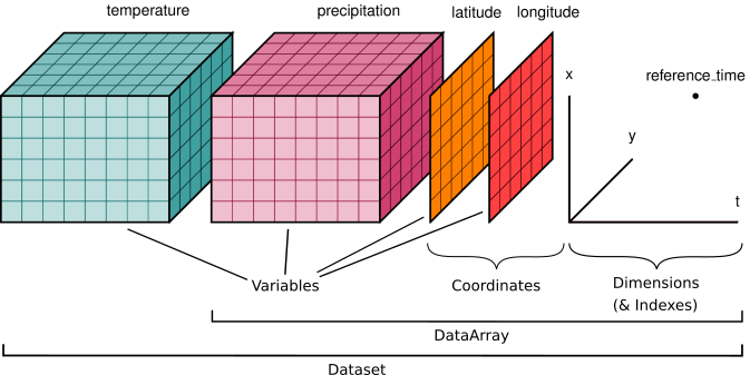
We’ll start by reviewing the various components of the Xarray data model, represented here visually:
import matplotlib.pyplot as plt
import numpy as np
import xarray as xr

xr.set_options(keep_attrs=True, display_expand_data=False)
np.set_printoptions(threshold=10, edgeitems=2)

%xmode minimal
%matplotlib inline
%config InlineBackend.figure_format='retina'
Exception reporting mode: Minimal
Xarray has a few small real-world tutorial datasets hosted in the xarray-data GitHub repository.
xarray.tutorial.load_dataset is a convenience function to download and open DataSets by name (listed at that link).
Here we’ll use air temperature from the National Center for Environmental Prediction. Xarray objects have convenient HTML representations to give an overview of what we’re working with:
ds = xr.tutorial.load_dataset("air_temperature")
ds
<xarray.Dataset> Size: 31MB
Dimensions:  (lat: 25, time: 2920, lon: 53)
Coordinates:
  * lat      (lat) float32 100B 75.0 72.5 70.0 67.5 65.0 ... 22.5 20.0 17.5 15.0
  * lon      (lon) float32 212B 200.0 202.5 205.0 207.5 ... 325.0 327.5 330.0
  * time     (time) datetime64[ns] 23kB 2013-01-01 ... 2014-12-31T18:00:00
Data variables:
    air      (time, lat, lon) float64 31MB 241.2 242.5 243.5 ... 296.2 295.7
Attributes:
    Conventions:  COARDS
    title:        4x daily NMC reanalysis (1948)
    description:  Data is from NMC initialized reanalysis\n(4x/day).  These a...
    platform:     Model
references: http://www.esrl.noaa.gov/psd/data/gridded/data.ncep.reanaly...Note that behind the scenes the tutorial.open_dataset downloads a file. It then uses xarray.open_dataset function to open that file (which for this datasets is a netCDF file).
A few things are done automatically upon opening, but controlled by keyword arguments. For example, try passing the keyword argument mask_and_scale=False… what happens?
What’s in a Dataset?#
Many DataArrays!
Datasets are dictionary-like containers of “DataArray”s. They are a mapping of variable name to DataArray:
# pull out "air" dataarray with dictionary syntax
ds["air"]
<xarray.DataArray 'air' (time: 2920, lat: 25, lon: 53)> Size: 31MB
241.2 242.5 243.5 244.0 244.1 243.9 ... 297.9 297.4 297.2 296.5 296.2 295.7
Coordinates:
* lat (lat) float32 100B 75.0 72.5 70.0 67.5 65.0 ... 22.5 20.0 17.5 15.0
* lon (lon) float32 212B 200.0 202.5 205.0 207.5 ... 325.0 327.5 330.0
* time (time) datetime64[ns] 23kB 2013-01-01 ... 2014-12-31T18:00:00
Attributes:
long_name: 4xDaily Air temperature at sigma level 995
units: degK
precision: 2
GRIB_id: 11
GRIB_name: TMP
var_desc: Air temperature
dataset: NMC Reanalysis
level_desc: Surface
statistic: Individual Obs
parent_stat: Other
actual_range: [185.16 322.1 ]You can save some typing by using the “attribute” or “dot” notation. This won’t
work for variable names that clash with a built-in method name (like mean for
example).
# pull out dataarray using dot notation
ds.air
<xarray.DataArray 'air' (time: 2920, lat: 25, lon: 53)> Size: 31MB
241.2 242.5 243.5 244.0 244.1 243.9 ... 297.9 297.4 297.2 296.5 296.2 295.7
Coordinates:
* lat (lat) float32 100B 75.0 72.5 70.0 67.5 65.0 ... 22.5 20.0 17.5 15.0
* lon (lon) float32 212B 200.0 202.5 205.0 207.5 ... 325.0 327.5 330.0
* time (time) datetime64[ns] 23kB 2013-01-01 ... 2014-12-31T18:00:00
Attributes:
long_name: 4xDaily Air temperature at sigma level 995
units: degK
precision: 2
GRIB_id: 11
GRIB_name: TMP
var_desc: Air temperature
dataset: NMC Reanalysis
level_desc: Surface
statistic: Individual Obs
parent_stat: Other
actual_range: [185.16 322.1 ]What’s in a DataArray?#
data + (a lot of) metadata
Name (optional)#
da = ds.air
da.name
'air'
Named dimensions#
.dims correspond to the axes of your data.
In this case we have 2 spatial dimensions (latitude and longitude are stored with shorthand names lat and lon) and one temporal dimension (time).
da.dims
('time', 'lat', 'lon')
Coordinate variables#
.coords is a simple data container
for coordinate variables.
Here we see the actual timestamps and spatial positions of our air temperature data:
da.coords
Coordinates:
* lat (lat) float32 100B 75.0 72.5 70.0 67.5 65.0 ... 22.5 20.0 17.5 15.0
* lon (lon) float32 212B 200.0 202.5 205.0 207.5 ... 325.0 327.5 330.0
* time (time) datetime64[ns] 23kB 2013-01-01 ... 2014-12-31T18:00:00
Coordinates objects support similar indexing notation
# extracting coordinate variables
da.lon
<xarray.DataArray 'lon' (lon: 53)> Size: 212B
200.0 202.5 205.0 207.5 210.0 212.5 ... 317.5 320.0 322.5 325.0 327.5 330.0
Coordinates:
* lon (lon) float32 212B 200.0 202.5 205.0 207.5 ... 325.0 327.5 330.0
Attributes:
standard_name: longitude
long_name: Longitude
units: degrees_east
axis: X# extracting coordinate variables from .coords
da.coords["lon"]
<xarray.DataArray 'lon' (lon: 53)> Size: 212B
200.0 202.5 205.0 207.5 210.0 212.5 ... 317.5 320.0 322.5 325.0 327.5 330.0
Coordinates:
* lon (lon) float32 212B 200.0 202.5 205.0 207.5 ... 325.0 327.5 330.0
Attributes:
standard_name: longitude
long_name: Longitude
units: degrees_east
axis: XIt is useful to think of the values in these coordinate variables as axis “labels” such as “tick labels” in a figure. These are coordinate locations on a grid at which you have data.
Arbitrary attributes#
.attrs is a dictionary that can contain arbitrary Python objects (strings, lists, integers, dictionaries, etc.) Your only
limitation is that some attributes may not be writeable to certain file formats.
da.attrs
{'long_name': '4xDaily Air temperature at sigma level 995',
'units': 'degK',
'precision': np.int16(2),
'GRIB_id': np.int16(11),
'GRIB_name': 'TMP',
'var_desc': 'Air temperature',
'dataset': 'NMC Reanalysis',
'level_desc': 'Surface',
'statistic': 'Individual Obs',
'parent_stat': 'Other',
'actual_range': array([185.16, 322.1 ], dtype=float32)}
# assign your own attributes!
da.attrs["who_is_awesome"] = "xarray"
da.attrs
{'long_name': '4xDaily Air temperature at sigma level 995',
'units': 'degK',
'precision': np.int16(2),
'GRIB_id': np.int16(11),
'GRIB_name': 'TMP',
'var_desc': 'Air temperature',
'dataset': 'NMC Reanalysis',
'level_desc': 'Surface',
'statistic': 'Individual Obs',
'parent_stat': 'Other',
'actual_range': array([185.16, 322.1 ], dtype=float32),
'who_is_awesome': 'xarray'}
da
<xarray.DataArray 'air' (time: 2920, lat: 25, lon: 53)> Size: 31MB
241.2 242.5 243.5 244.0 244.1 243.9 ... 297.9 297.4 297.2 296.5 296.2 295.7
Coordinates:
* lat (lat) float32 100B 75.0 72.5 70.0 67.5 65.0 ... 22.5 20.0 17.5 15.0
* lon (lon) float32 212B 200.0 202.5 205.0 207.5 ... 325.0 327.5 330.0
* time (time) datetime64[ns] 23kB 2013-01-01 ... 2014-12-31T18:00:00
Attributes:
long_name: 4xDaily Air temperature at sigma level 995
units: degK
precision: 2
GRIB_id: 11
GRIB_name: TMP
var_desc: Air temperature
dataset: NMC Reanalysis
level_desc: Surface
statistic: Individual Obs
parent_stat: Other
actual_range: [185.16 322.1 ]
who_is_awesome: xarrayUnderlying data#
.data contains the numpy array storing air temperature values.
Xarray structures wrap underlying simpler array-like data structures. This part of Xarray is quite extensible allowing for distributed array, GPU arrays, sparse arrays, arrays with units etc. We’ll briefly look at this later in this tutorial.
da.data
array([[[241.2 , 242.5 , ..., 235.5 , 238.6 ],
        [243.8 , 244.5 , ..., 235.3 , 239.3 ],
        ...,
        [295.9 , 296.2 , ..., 295.9 , 295.2 ],
        [296.29, 296.79, ..., 296.79, 296.6 ]],

       [[242.1 , 242.7 , ..., 233.6 , 235.8 ],
        [243.6 , 244.1 , ..., 232.5 , 235.7 ],
        ...,
        [296.2 , 296.7 , ..., 295.5 , 295.1 ],
        [296.29, 297.2 , ..., 296.4 , 296.6 ]],

       ...,

       [[245.79, 244.79, ..., 243.99, 244.79],
        [249.89, 249.29, ..., 242.49, 244.29],
        ...,
        [296.29, 297.19, ..., 295.09, 294.39],
        [297.79, 298.39, ..., 295.49, 295.19]],

       [[245.09, 244.29, ..., 241.49, 241.79],
        [249.89, 249.29, ..., 240.29, 241.69],
        ...,
        [296.09, 296.89, ..., 295.69, 295.19],
        [297.69, 298.09, ..., 296.19, 295.69]]])
# what is the type of the underlying data
type(da.data)
numpy.ndarray
Review#
Xarray provides two main data structures:
DataArraysthat wrap underlying data containers (e.g. numpy arrays) and contain associated metadataDatasetsthat are dictionary-like containers of DataArrays
DataArrays contain underlying arrays and associated metadata:
Name
Dimension names
Coordinate variables
and arbitrary attributes.
Why Xarray?#
Metadata provides context and provides code that is more legible. This reduces the likelihood of errors from typos and makes analysis more intuitive and fun!
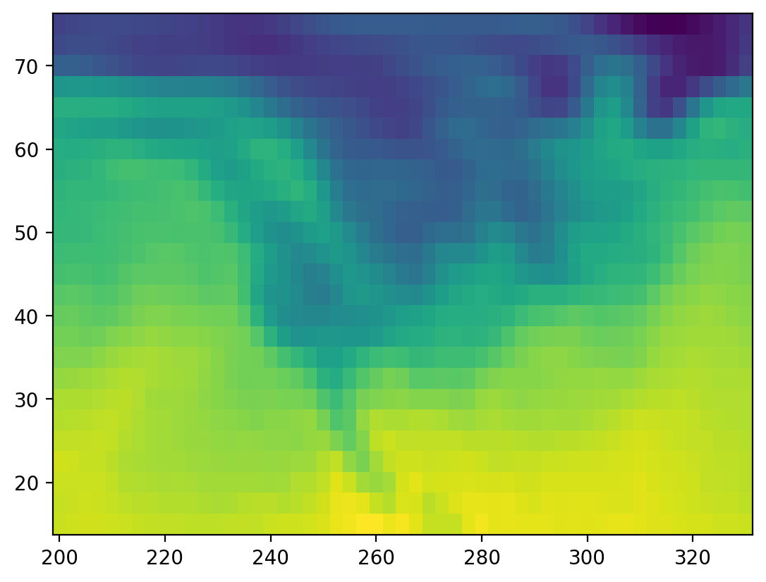
Analysis without xarray: X(#
# plot the first timestep
lat = ds.air.lat.data # numpy array
lon = ds.air.lon.data # numpy array
temp = ds.air.data # numpy array
plt.figure()
plt.pcolormesh(lon, lat, temp[0, :, :]);
temp.mean(axis=1) ## what did I just do? I can't tell by looking at this line.
array([[279.398 , 279.6664, ..., 280.3152, 280.6624],
[279.0572, 279.538 , ..., 280.27 , 280.7976],
...,
[279.398 , 279.666 , ..., 280.342 , 280.834 ],
[279.27 , 279.354 , ..., 279.97 , 280.482 ]])
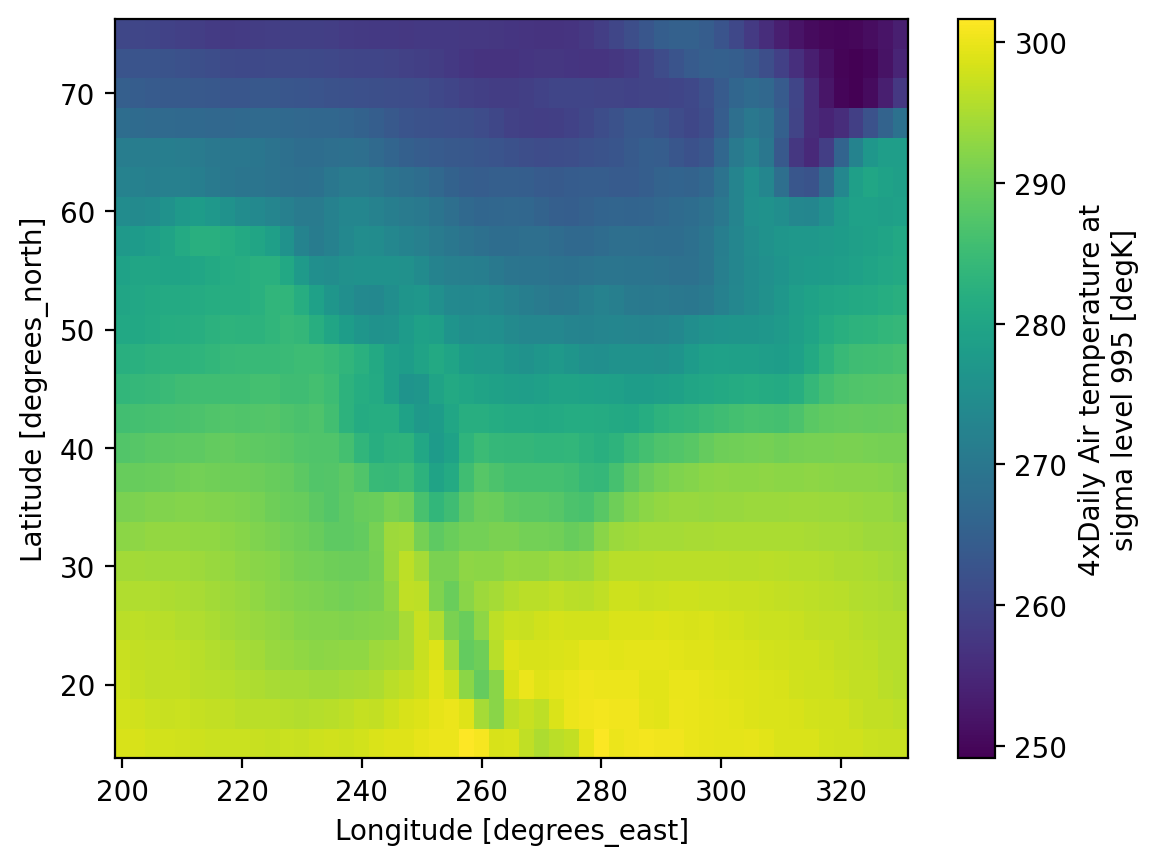
Analysis with xarray =)#
How readable is this code?
ds.air.isel(time=0).plot(x="lon");

Use dimension names instead of axis numbers
ds.air.mean(dim="time").plot(x="lon")
<matplotlib.collections.QuadMesh at 0x7f2ff96e3920>
Extracting data or “indexing”#
Xarray supports
label-based indexing using
.selposition-based indexing using
.isel
See the user guide for more.
Label-based indexing#
Xarray inherits its label-based indexing rules from pandas; this means great support for dates and times!
# here's what ds looks like
ds
<xarray.Dataset> Size: 31MB
Dimensions: (lat: 25, time: 2920, lon: 53)
Coordinates:
* lat (lat) float32 100B 75.0 72.5 70.0 67.5 65.0 ... 22.5 20.0 17.5 15.0
* lon (lon) float32 212B 200.0 202.5 205.0 207.5 ... 325.0 327.5 330.0
* time (time) datetime64[ns] 23kB 2013-01-01 ... 2014-12-31T18:00:00
Data variables:
air (time, lat, lon) float64 31MB 241.2 242.5 243.5 ... 296.2 295.7
Attributes:
Conventions: COARDS
title: 4x daily NMC reanalysis (1948)
description: Data is from NMC initialized reanalysis\n(4x/day). These a...
platform: Model
references: http://www.esrl.noaa.gov/psd/data/gridded/data.ncep.reanaly...# pull out data for all of 2013-May
ds.sel(time="2013-05")
<xarray.Dataset> Size: 1MB
Dimensions: (lat: 25, time: 124, lon: 53)
Coordinates:
* lat (lat) float32 100B 75.0 72.5 70.0 67.5 65.0 ... 22.5 20.0 17.5 15.0
* lon (lon) float32 212B 200.0 202.5 205.0 207.5 ... 325.0 327.5 330.0
* time (time) datetime64[ns] 992B 2013-05-01 ... 2013-05-31T18:00:00
Data variables:
air (time, lat, lon) float64 1MB 259.2 259.3 259.1 ... 297.6 297.5
Attributes:
Conventions: COARDS
title: 4x daily NMC reanalysis (1948)
description: Data is from NMC initialized reanalysis\n(4x/day). These a...
platform: Model
references: http://www.esrl.noaa.gov/psd/data/gridded/data.ncep.reanaly...# demonstrate slicing
ds.sel(time=slice("2013-05", "2013-07"))
<xarray.Dataset> Size: 4MB
Dimensions: (lat: 25, time: 368, lon: 53)
Coordinates:
* lat (lat) float32 100B 75.0 72.5 70.0 67.5 65.0 ... 22.5 20.0 17.5 15.0
* lon (lon) float32 212B 200.0 202.5 205.0 207.5 ... 325.0 327.5 330.0
* time (time) datetime64[ns] 3kB 2013-05-01 ... 2013-07-31T18:00:00
Data variables:
air (time, lat, lon) float64 4MB 259.2 259.3 259.1 ... 299.5 299.7
Attributes:
Conventions: COARDS
title: 4x daily NMC reanalysis (1948)
description: Data is from NMC initialized reanalysis\n(4x/day). These a...
platform: Model
references: http://www.esrl.noaa.gov/psd/data/gridded/data.ncep.reanaly...ds.sel(time="2013")
<xarray.Dataset> Size: 15MB
Dimensions: (lat: 25, time: 1460, lon: 53)
Coordinates:
* lat (lat) float32 100B 75.0 72.5 70.0 67.5 65.0 ... 22.5 20.0 17.5 15.0
* lon (lon) float32 212B 200.0 202.5 205.0 207.5 ... 325.0 327.5 330.0
* time (time) datetime64[ns] 12kB 2013-01-01 ... 2013-12-31T18:00:00
Data variables:
air (time, lat, lon) float64 15MB 241.2 242.5 243.5 ... 295.1 294.7
Attributes:
Conventions: COARDS
title: 4x daily NMC reanalysis (1948)
description: Data is from NMC initialized reanalysis\n(4x/day). These a...
platform: Model
references: http://www.esrl.noaa.gov/psd/data/gridded/data.ncep.reanaly...# demonstrate "nearest" indexing
ds.sel(lon=240.2, method="nearest")
<xarray.Dataset> Size: 607kB
Dimensions: (lat: 25, time: 2920)
Coordinates:
* lat (lat) float32 100B 75.0 72.5 70.0 67.5 65.0 ... 22.5 20.0 17.5 15.0
lon float32 4B 240.0
* time (time) datetime64[ns] 23kB 2013-01-01 ... 2014-12-31T18:00:00
Data variables:
air (time, lat) float64 584kB 239.6 237.2 240.1 ... 294.8 296.9 298.4
Attributes:
Conventions: COARDS
title: 4x daily NMC reanalysis (1948)
description: Data is from NMC initialized reanalysis\n(4x/day). These a...
platform: Model
references: http://www.esrl.noaa.gov/psd/data/gridded/data.ncep.reanaly...# "nearest indexing at multiple points"
ds.sel(lon=[240.125, 234], lat=[40.3, 50.3], method="nearest")
<xarray.Dataset> Size: 117kB
Dimensions: (lat: 2, time: 2920, lon: 2)
Coordinates:
* lat (lat) float32 8B 40.0 50.0
* lon (lon) float32 8B 240.0 235.0
* time (time) datetime64[ns] 23kB 2013-01-01 ... 2014-12-31T18:00:00
Data variables:
air (time, lat, lon) float64 93kB 268.1 283.0 265.5 ... 256.8 268.6
Attributes:
Conventions: COARDS
title: 4x daily NMC reanalysis (1948)
description: Data is from NMC initialized reanalysis\n(4x/day). These a...
platform: Model
references: http://www.esrl.noaa.gov/psd/data/gridded/data.ncep.reanaly...Position-based indexing#
This is similar to your usual numpy array[0, 2, 3] but with the power of named
dimensions!
ds.air.data[0, 2, 3]
np.float64(247.5)
# pull out time index 0, lat index 2, and lon index 3
ds.air.isel(time=0, lat=2, lon=3) # much better than ds.air[0, 2, 3]
<xarray.DataArray 'air' ()> Size: 8B
247.5
Coordinates:
lat float32 4B 70.0
lon float32 4B 207.5
time datetime64[ns] 8B 2013-01-01
Attributes:
long_name: 4xDaily Air temperature at sigma level 995
units: degK
precision: 2
GRIB_id: 11
GRIB_name: TMP
var_desc: Air temperature
dataset: NMC Reanalysis
level_desc: Surface
statistic: Individual Obs
parent_stat: Other
actual_range: [185.16 322.1 ]
who_is_awesome: xarray# demonstrate slicing
ds.air.isel(lat=slice(10))
<xarray.DataArray 'air' (time: 2920, lat: 10, lon: 53)> Size: 12MB
241.2 242.5 243.5 244.0 244.1 243.9 ... 273.4 273.8 273.5 273.8 275.0 276.2
Coordinates:
* lat (lat) float32 40B 75.0 72.5 70.0 67.5 65.0 62.5 60.0 57.5 55.0 52.5
* lon (lon) float32 212B 200.0 202.5 205.0 207.5 ... 325.0 327.5 330.0
* time (time) datetime64[ns] 23kB 2013-01-01 ... 2014-12-31T18:00:00
Attributes:
long_name: 4xDaily Air temperature at sigma level 995
units: degK
precision: 2
GRIB_id: 11
GRIB_name: TMP
var_desc: Air temperature
dataset: NMC Reanalysis
level_desc: Surface
statistic: Individual Obs
parent_stat: Other
actual_range: [185.16 322.1 ]
who_is_awesome: xarrayConcepts for computation#
Consider calculating the mean air temperature per unit surface area for this dataset. Because latitude and longitude correspond to spherical coordinates for Earth’s surface, each 2.5x2.5 degree grid cell actually has a different surface area as you move away from the equator! This is because latitudinal length is fixed ($ \delta Lat = R \delta \phi $), but longitudinal length varies with latitude ($ \delta Lon = R \delta \lambda \cos(\phi) $)
So the area element for lat-lon coordinates is
$$ \delta A = R^2 \delta\phi , \delta\lambda \cos(\phi) $$
where $\phi$ is latitude, $\delta \phi$ is the spacing of the points in latitude, $\delta \lambda$ is the spacing of the points in longitude, and $R$ is Earth’s radius. (In this formula, $\phi$ and $\lambda$ are measured in radians)
# Earth's average radius in meters
R = 6.371e6
# Coordinate spacing for this dataset is 2.5 x 2.5 degrees
dϕ = np.deg2rad(2.5)
dλ = np.deg2rad(2.5)
dlat = R * dϕ * xr.ones_like(ds.air.lon)
dlon = R * dλ * np.cos(np.deg2rad(ds.air.lat))
dlon.name = "dlon"
dlat.name = "dlat"
There are two concepts here:
you can call functions like
np.cosandnp.deg2rad(“numpy ufuncs”) on Xarray objects and receive an Xarray object back.We used ones_like to create a DataArray that looks like
ds.air.lonin all respects, except that the data are all ones
# returns an xarray DataArray!
np.cos(np.deg2rad(ds.lat))
<xarray.DataArray 'lat' (lat: 25)> Size: 100B
0.2588 0.3007 0.342 0.3827 0.4226 0.4617 ... 0.9063 0.9239 0.9397 0.9537 0.9659
Coordinates:
* lat (lat) float32 100B 75.0 72.5 70.0 67.5 65.0 ... 22.5 20.0 17.5 15.0
Attributes:
standard_name: latitude
long_name: Latitude
units: degrees_north
axis: Y# cell latitude length is constant with longitude
dlat
<xarray.DataArray 'dlat' (lon: 53)> Size: 424B
2.78e+05 2.78e+05 2.78e+05 2.78e+05 ... 2.78e+05 2.78e+05 2.78e+05 2.78e+05
Coordinates:
* lon (lon) float32 212B 200.0 202.5 205.0 207.5 ... 325.0 327.5 330.0
Attributes:
standard_name: longitude
long_name: Longitude
units: degrees_east
axis: X# cell longitude length changes with latitude
dlon
<xarray.DataArray 'dlon' (lat: 25)> Size: 200B
7.195e+04 8.359e+04 9.508e+04 1.064e+05 ... 2.612e+05 2.651e+05 2.685e+05
Coordinates:
* lat (lat) float32 100B 75.0 72.5 70.0 67.5 65.0 ... 22.5 20.0 17.5 15.0
Attributes:
standard_name: latitude
long_name: Latitude
units: degrees_north
axis: YBroadcasting: expanding data#
Our longitude and latitude length DataArrays are both 1D with different dimension names. If we multiple these DataArrays together the dimensionality is expanded to 2D by broadcasting:
cell_area = dlon * dlat
cell_area
<xarray.DataArray (lat: 25, lon: 53)> Size: 11kB
2e+10 2e+10 2e+10 2e+10 2e+10 ... 7.464e+10 7.464e+10 7.464e+10 7.464e+10
Coordinates:
* lat (lat) float32 100B 75.0 72.5 70.0 67.5 65.0 ... 22.5 20.0 17.5 15.0
* lon (lon) float32 212B 200.0 202.5 205.0 207.5 ... 325.0 327.5 330.0
Attributes:
standard_name: latitude
long_name: Latitude
units: degrees_north
axis: YThe result has two dimensions because xarray realizes that dimensions lon and
lat are different so it automatically “broadcasts” to get a 2D result. See the
last row in this image from Jake VanderPlas Python Data Science Handbook
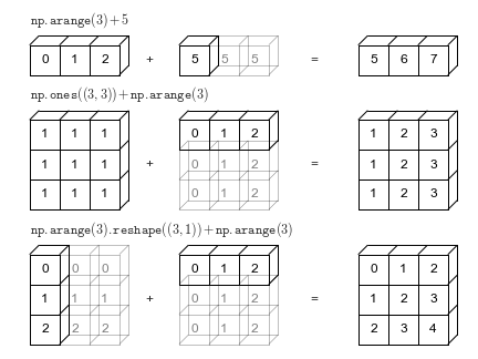
Because xarray knows about dimension names we avoid having to create unnecessary
size-1 dimensions using np.newaxis or .reshape. For more, see the user guide
Alignment: putting data on the same grid#
When doing arithmetic operations xarray automatically “aligns” i.e. puts the
data on the same grid. In this case cell_area and ds.air are at the same
lat, lon points we end up with a result with the same shape (25x53):
ds.air.isel(time=1) / cell_area
<xarray.DataArray (lat: 25, lon: 53)> Size: 11kB
1.21e-08 1.213e-08 1.215e-08 1.217e-08 ... 3.971e-09 3.971e-09 3.974e-09
Coordinates:
* lat (lat) float32 100B 75.0 72.5 70.0 67.5 65.0 ... 22.5 20.0 17.5 15.0
* lon (lon) float32 212B 200.0 202.5 205.0 207.5 ... 325.0 327.5 330.0
time datetime64[ns] 8B 2013-01-01T06:00:00
Attributes:
long_name: 4xDaily Air temperature at sigma level 995
units: degK
precision: 2
GRIB_id: 11
GRIB_name: TMP
var_desc: Air temperature
dataset: NMC Reanalysis
level_desc: Surface
statistic: Individual Obs
parent_stat: Other
actual_range: [185.16 322.1 ]
who_is_awesome: xarrayNow lets make cell_area unaligned i.e. change the coordinate labels
# make a copy of cell_area
# then add 1e-5 degrees to latitude
cell_area_bad = cell_area.copy(deep=True)
cell_area_bad["lat"] = cell_area.lat + 1e-5 # latitudes are off by 1e-5 degrees!
cell_area_bad
<xarray.DataArray (lat: 25, lon: 53)> Size: 11kB
2e+10 2e+10 2e+10 2e+10 2e+10 ... 7.464e+10 7.464e+10 7.464e+10 7.464e+10
Coordinates:
* lon (lon) float32 212B 200.0 202.5 205.0 207.5 ... 325.0 327.5 330.0
* lat (lat) float32 100B 75.0 72.5 70.0 67.5 65.0 ... 22.5 20.0 17.5 15.0
Attributes:
standard_name: latitude
long_name: Latitude
units: degrees_north
axis: Ycell_area_bad * ds.air.isel(time=1)
<xarray.DataArray (lat: 0, lon: 53)> Size: 0B
Coordinates:
* lon (lon) float32 212B 200.0 202.5 205.0 207.5 ... 325.0 327.5 330.0
* lat (lat) float32 0B
time datetime64[ns] 8B 2013-01-01T06:00:00
Attributes:
standard_name: latitude
long_name: Latitude
units: degrees_north
axis: YThe result is an empty array with no latitude coordinates because none of them were aligned!
Tip
If you notice extra NaNs or missing points after xarray computation, it means that your xarray coordinates were not aligned exactly.
To make sure variables are aligned as you think they are, do the following:
xr.align(cell_area_bad, ds.air, join="exact")
ValueError: cannot align objects with join='exact' where index/labels/sizes are not equal along these coordinates (dimensions): 'lat' ('lat',)
The above statement raises an error since the two are not aligned.
See also
For more, see the Xarray documentation. This tutorial notebook also covers alignment and broadcasting (highly recommended)
High level computation#
(groupby, resample, rolling, coarsen, weighted)
Xarray has some very useful high level objects that let you do common computations:
groupby: Bin data in to groups and reduceresample: Groupby specialized for time axes. Either downsample or upsample your data.rolling: Operate on rolling windows of your data e.g. running meancoarsen: Downsample your dataweighted: Weight your data before reducing
Below we quickly demonstrate these patterns. See the user guide links above and the tutorial for more.
groupby#
# here's ds
ds
<xarray.Dataset> Size: 31MB
Dimensions: (lat: 25, time: 2920, lon: 53)
Coordinates:
* lat (lat) float32 100B 75.0 72.5 70.0 67.5 65.0 ... 22.5 20.0 17.5 15.0
* lon (lon) float32 212B 200.0 202.5 205.0 207.5 ... 325.0 327.5 330.0
* time (time) datetime64[ns] 23kB 2013-01-01 ... 2014-12-31T18:00:00
Data variables:
air (time, lat, lon) float64 31MB 241.2 242.5 243.5 ... 296.2 295.7
Attributes:
Conventions: COARDS
title: 4x daily NMC reanalysis (1948)
description: Data is from NMC initialized reanalysis\n(4x/day). These a...
platform: Model
references: http://www.esrl.noaa.gov/psd/data/gridded/data.ncep.reanaly...# seasonal groups
ds.groupby("time.season")
<DatasetGroupBy, grouped over 1 grouper(s), 4 groups in total:
'season': 4/4 groups present with labels 'DJF', 'JJA', 'MAM', 'SON'>
# make a seasonal mean
seasonal_mean = ds.groupby("time.season").mean()
seasonal_mean
<xarray.Dataset> Size: 43kB
Dimensions: (season: 4, lat: 25, lon: 53)
Coordinates:
* lat (lat) float32 100B 75.0 72.5 70.0 67.5 65.0 ... 22.5 20.0 17.5 15.0
* lon (lon) float32 212B 200.0 202.5 205.0 207.5 ... 325.0 327.5 330.0
* season (season) object 32B 'DJF' 'JJA' 'MAM' 'SON'
Data variables:
air (season, lat, lon) float64 42kB 247.0 247.0 246.7 ... 299.4 299.5
Attributes:
Conventions: COARDS
title: 4x daily NMC reanalysis (1948)
description: Data is from NMC initialized reanalysis\n(4x/day). These a...
platform: Model
references: http://www.esrl.noaa.gov/psd/data/gridded/data.ncep.reanaly...The seasons are out of order (they are alphabetically sorted). This is a common
annoyance. The solution is to use .sel to change the order of labels
seasonal_mean = seasonal_mean.sel(season=["DJF", "MAM", "JJA", "SON"])
seasonal_mean
<xarray.Dataset> Size: 43kB
Dimensions: (season: 4, lat: 25, lon: 53)
Coordinates:
* lat (lat) float32 100B 75.0 72.5 70.0 67.5 65.0 ... 22.5 20.0 17.5 15.0
* lon (lon) float32 212B 200.0 202.5 205.0 207.5 ... 325.0 327.5 330.0
* season (season) object 32B 'DJF' 'MAM' 'JJA' 'SON'
Data variables:
air (season, lat, lon) float64 42kB 247.0 247.0 246.7 ... 299.4 299.5
Attributes:
Conventions: COARDS
title: 4x daily NMC reanalysis (1948)
description: Data is from NMC initialized reanalysis\n(4x/day). These a...
platform: Model
references: http://www.esrl.noaa.gov/psd/data/gridded/data.ncep.reanaly...seasonal_mean.air.plot(col="season")
<xarray.plot.facetgrid.FacetGrid at 0x7f2ff8221640>
resample#
# resample to monthly frequency
ds.resample(time="M").mean()
/home/eric/miniconda3/envs/uwgda2025/lib/python3.12/site-packages/xarray/groupers.py:487: FutureWarning: 'M' is deprecated and will be removed in a future version, please use 'ME' instead.
self.index_grouper = pd.Grouper(
<xarray.Dataset> Size: 255kB
Dimensions: (time: 24, lat: 25, lon: 53)
Coordinates:
* lat (lat) float32 100B 75.0 72.5 70.0 67.5 65.0 ... 22.5 20.0 17.5 15.0
* lon (lon) float32 212B 200.0 202.5 205.0 207.5 ... 325.0 327.5 330.0
* time (time) datetime64[ns] 192B 2013-01-31 2013-02-28 ... 2014-12-31
Data variables:
air (time, lat, lon) float64 254kB 244.5 244.7 244.7 ... 297.7 297.7
Attributes:
Conventions: COARDS
title: 4x daily NMC reanalysis (1948)
description: Data is from NMC initialized reanalysis\n(4x/day). These a...
platform: Model
references: http://www.esrl.noaa.gov/psd/data/gridded/data.ncep.reanaly...weighted#
# weight by cell_area and take mean over (time, lon)
ds.weighted(cell_area).mean(["lon", "time"]).air.plot(y="lat");
Visualization#
(.plot)
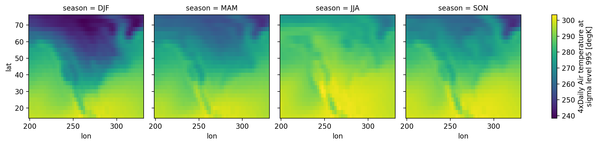
We have seen very simple plots earlier. Xarray also lets you easily visualize 3D and 4D datasets by presenting multiple facets (or panels or subplots) showing variations across rows and/or columns.
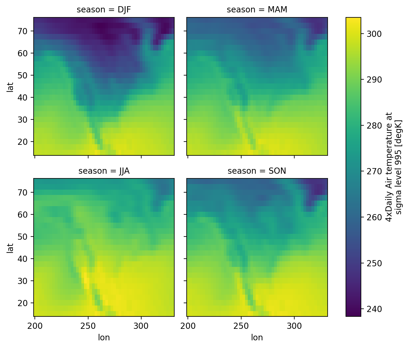
# facet the seasonal_mean
seasonal_mean.air.plot(col="season", col_wrap=2);
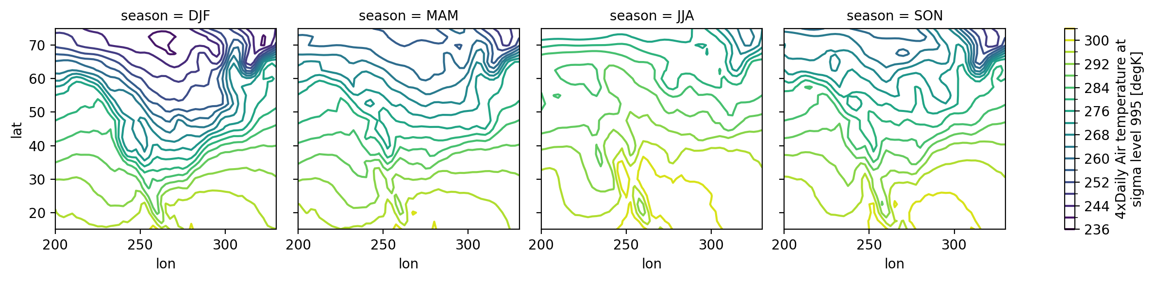
# contours
seasonal_mean.air.plot.contour(col="season", levels=20, add_colorbar=True);
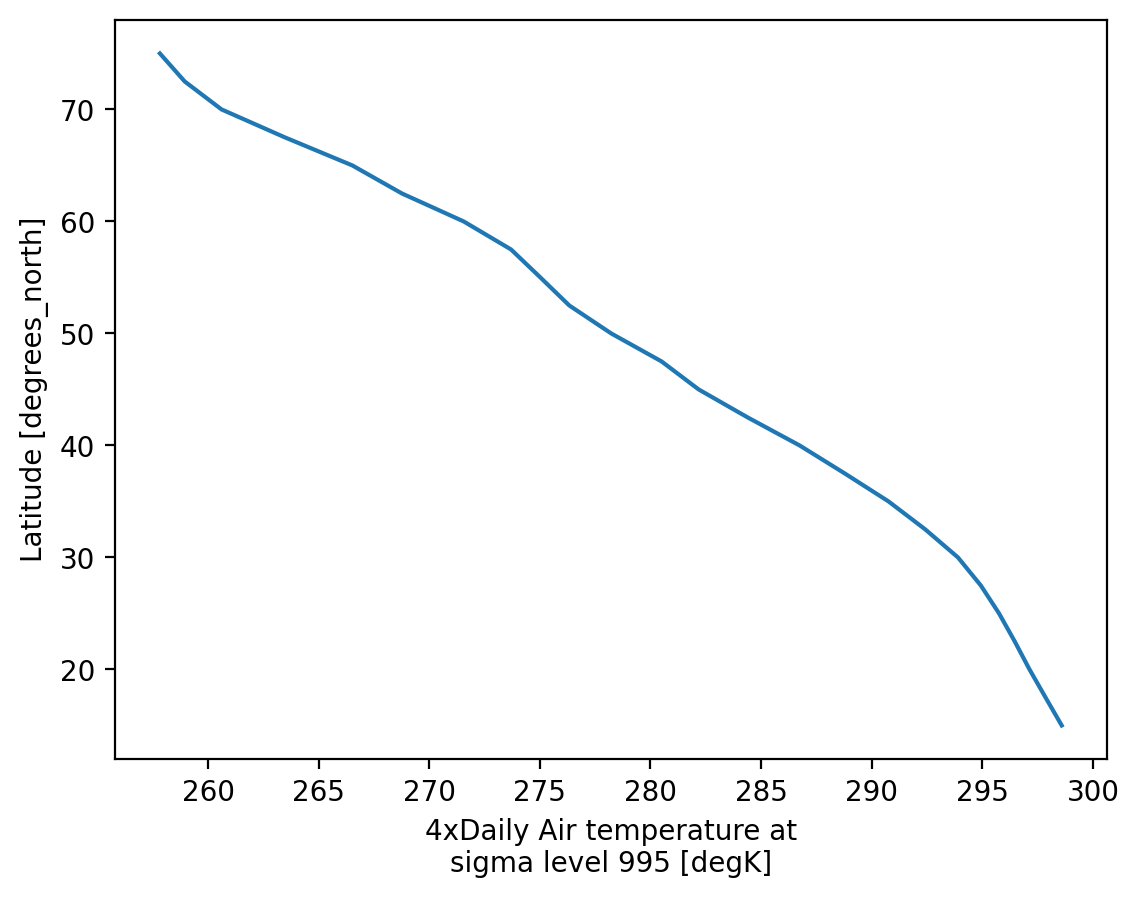
# line plots too? wut
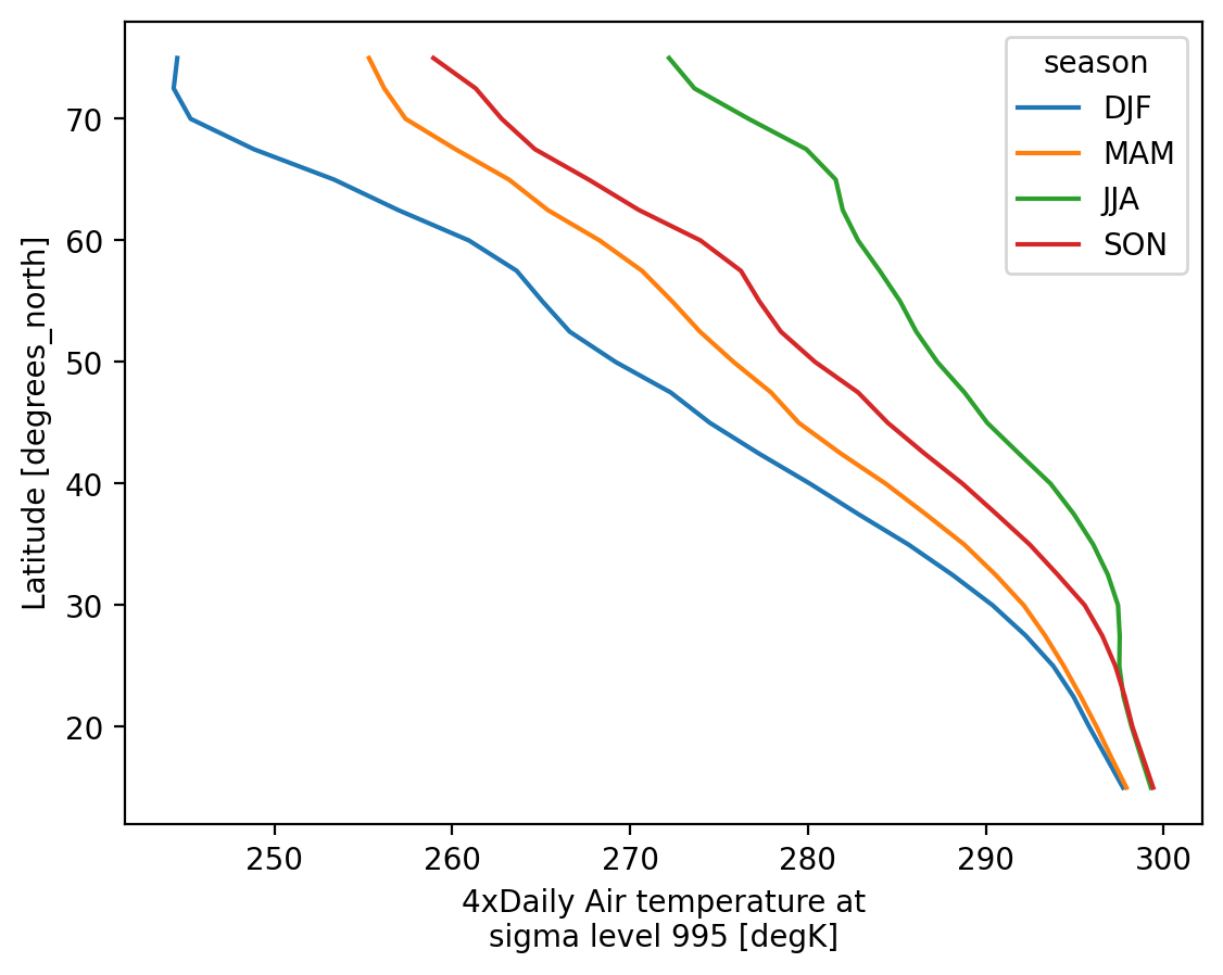
seasonal_mean.air.mean("lon").plot.line(hue="season", y="lat");
For more see the user guide, the gallery, and the tutorial material.
Band math / convert variables#
We’re in degrees Kelvin, let’s practice converting!
ds["air"]
<xarray.DataArray 'air' (time: 2920, lat: 25, lon: 53)> Size: 31MB
241.2 242.5 243.5 244.0 244.1 243.9 ... 297.9 297.4 297.2 296.5 296.2 295.7
Coordinates:
  * lat      (lat) float32 100B 75.0 72.5 70.0 67.5 65.0 ... 22.5 20.0 17.5 15.0
  * lon      (lon) float32 212B 200.0 202.5 205.0 207.5 ... 325.0 327.5 330.0
  * time     (time) datetime64[ns] 23kB 2013-01-01 ... 2014-12-31T18:00:00
Attributes:
    long_name:     4xDaily Air temperature at sigma level 995
    units:         degK
    precision:     2
    GRIB_id:       11
    GRIB_name:     TMP
    var_desc:      Air temperature
    dataset:       NMC Reanalysis
    level_desc:    Surface
    statistic:     Individual Obs
    parent_stat:   Other
    actual_range:  [185.16 322.1 ]
who_is_awesome: xarrayds["air"].attrs
{'long_name': '4xDaily Air temperature at sigma level 995',
'units': 'degK',
'precision': np.int16(2),
'GRIB_id': np.int16(11),
'GRIB_name': 'TMP',
'var_desc': 'Air temperature',
'dataset': 'NMC Reanalysis',
'level_desc': 'Surface',
'statistic': 'Individual Obs',
'parent_stat': 'Other',
'actual_range': array([185.16, 322.1 ], dtype=float32),
'who_is_awesome': 'xarray'}
Notice these nice attributes on the air variable! If we convert away from Kelvin, we should probbaly update the units attribute for good bookeeping!
ds["air"] = ds["air"] - 273.15
ds["air"].attrs["units"] = "Celsius"
ds
<xarray.Dataset> Size: 31MB
Dimensions: (lat: 25, time: 2920, lon: 53)
Coordinates:
  * lat      (lat) float32 100B 75.0 72.5 70.0 67.5 65.0 ... 22.5 20.0 17.5 15.0
  * lon      (lon) float32 212B 200.0 202.5 205.0 207.5 ... 325.0 327.5 330.0
  * time     (time) datetime64[ns] 23kB 2013-01-01 ... 2014-12-31T18:00:00
Data variables:
air (time, lat, lon) float64 31MB -31.95 -30.65 -29.65 ... 23.04 22.54
Attributes:
Conventions: COARDS
title: 4x daily NMC reanalysis (1948)
description: Data is from NMC initialized reanalysis\n(4x/day). These a...
platform: Model
references: http://www.esrl.noaa.gov/psd/data/gridded/data.ncep.reanaly...ds["air"].isel(time=0).plot(cmap="viridis")
<matplotlib.collections.QuadMesh at 0x7f2ff81a57f0>
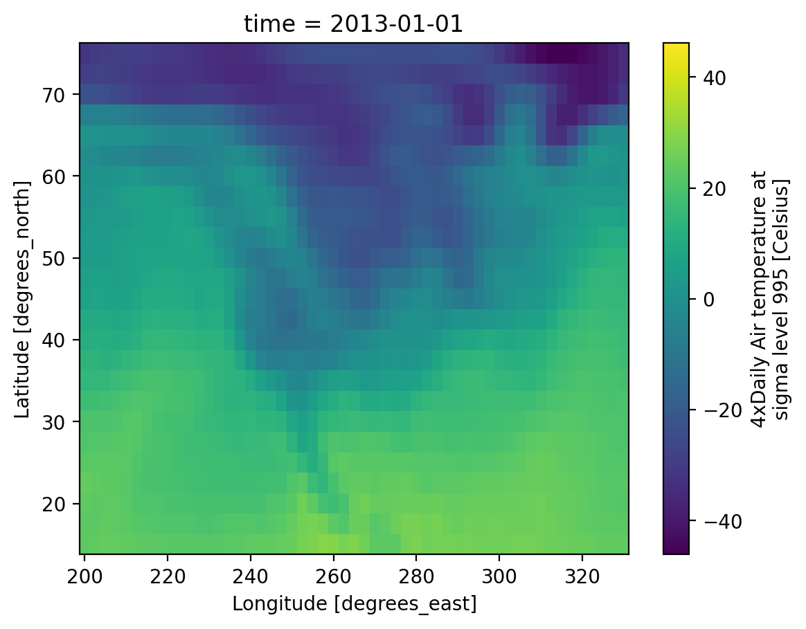
That’s great, the plot also has updated units! Now what if we had a friend that couldn’t interpret Celsius easily?? To Fahrenheit…
ds["air"] = ds["air"] * (9/5) + 32
ds["air"].attrs["units"] = "Fahrenheit"
ds
<xarray.Dataset> Size: 31MB
Dimensions: (lat: 25, time: 2920, lon: 53)
Coordinates:
* lat (lat) float32 100B 75.0 72.5 70.0 67.5 65.0 ... 22.5 20.0 17.5 15.0
* lon (lon) float32 212B 200.0 202.5 205.0 207.5 ... 325.0 327.5 330.0
* time (time) datetime64[ns] 23kB 2013-01-01 ... 2014-12-31T18:00:00
Data variables:
air (time, lat, lon) float64 31MB -25.51 -23.17 -21.37 ... 73.47 72.57
Attributes:
Conventions: COARDS
title: 4x daily NMC reanalysis (1948)
description: Data is from NMC initialized reanalysis\n(4x/day). These a...
platform: Model
references: http://www.esrl.noaa.gov/psd/data/gridded/data.ncep.reanaly...So let’s show the mean temperature in Fahrenheit for 2013…
f,axs=plt.subplots(1,2,figsize=(12,4))
ds["air"].sel(time="2013").mean(dim="time").plot.imshow(ax=axs[0], cmap="viridis")
ds["air"].sel(time="2013").mean(dim="time").plot.imshow(ax=axs[1], cmap="viridis",robust=True)
f.tight_layout()
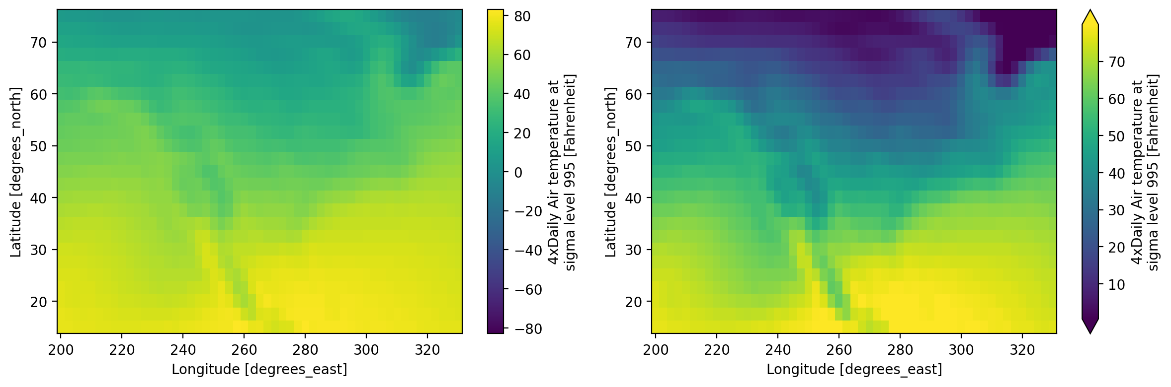
What does robust=True in the .plot.imshow() call do again?
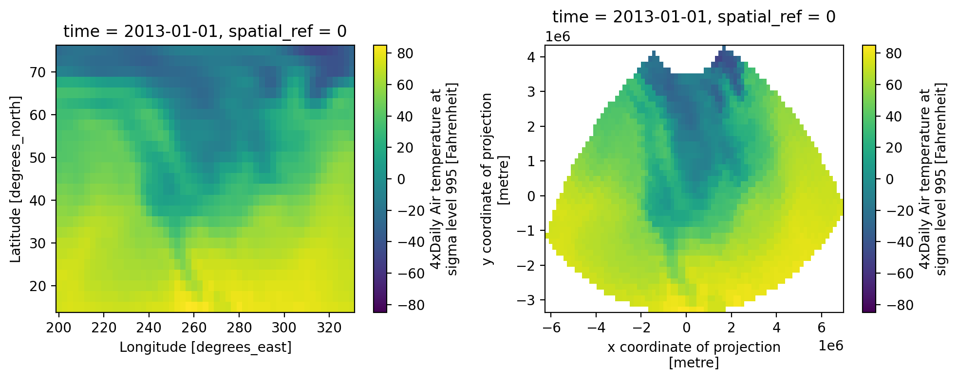
Reprojection and clipping#
Since rioxarray extends Xarray DataArray and Dataset objects, we can use our favorite rioxarray functions using the .rio accessor like we’ve done before!
ds = ds.rio.write_crs("EPSG:4326")
ds
<xarray.Dataset> Size: 31MB
Dimensions: (lat: 25, time: 2920, lon: 53)
Coordinates:
* lat (lat) float32 100B 75.0 72.5 70.0 67.5 ... 22.5 20.0 17.5 15.0
* lon (lon) float32 212B 200.0 202.5 205.0 ... 325.0 327.5 330.0
* time (time) datetime64[ns] 23kB 2013-01-01 ... 2014-12-31T18:00:00
spatial_ref int64 8B 0
Data variables:
air (time, lat, lon) float64 31MB -25.51 -23.17 ... 73.47 72.57
Attributes:
Conventions: COARDS
title: 4x daily NMC reanalysis (1948)
description: Data is from NMC initialized reanalysis\n(4x/day). These a...
platform: Model
references: http://www.esrl.noaa.gov/psd/data/gridded/data.ncep.reanaly...ds.rio.crs
CRS.from_wkt('GEOGCS["WGS 84",DATUM["WGS_1984",SPHEROID["WGS 84",6378137,298.257223563,AUTHORITY["EPSG","7030"]],AUTHORITY["EPSG","6326"]],PRIMEM["Greenwich",0,AUTHORITY["EPSG","8901"]],UNIT["degree",0.0174532925199433,AUTHORITY["EPSG","9122"]],AXIS["Latitude",NORTH],AXIS["Longitude",EAST],AUTHORITY["EPSG","4326"]]')
projected_ds = ds.rio.reproject("EPSG:2163")
projected_ds
<xarray.Dataset> Size: 89MB
Dimensions: (x: 81, y: 47, time: 2920)
Coordinates:
* x (x) float64 648B -6.192e+06 -6.028e+06 ... 6.735e+06 6.898e+06
* y (y) float64 376B 4.247e+06 4.084e+06 ... -3.116e+06 -3.28e+06
* time (time) datetime64[ns] 23kB 2013-01-01 ... 2014-12-31T18:00:00
spatial_ref int64 8B 0
Data variables:
air (time, y, x) float64 89MB nan nan nan nan ... nan nan nan nan
Attributes:
Conventions: COARDS
title: 4x daily NMC reanalysis (1948)
description: Data is from NMC initialized reanalysis\n(4x/day). These a...
platform: Model
references: http://www.esrl.noaa.gov/psd/data/gridded/data.ncep.reanaly...f,axs=plt.subplots(1,2,figsize=(10,4))
ds["air"].isel(time=0).plot.imshow(ax=axs[0],cmap="viridis")
projected_ds["air"].isel(time=0).plot.imshow(ax=axs[1],cmap="viridis")
f.tight_layout()
import geopandas as gpd
states_gdf = gpd.read_file('http://eric.clst.org/assets/wiki/uploads/Stuff/gz_2010_us_040_00_5m.json')
states_projected_gdf = states_gdf.to_crs(projected_ds.rio.crs)
wa_projected_gdf = states_projected_gdf[states_projected_gdf["NAME"] == "Washington"]
tx_projected_gdf = states_projected_gdf[states_projected_gdf["NAME"] == "Texas"]
wa_projected_and_clipped_ds = projected_ds.rio.clip(wa_projected_gdf.geometry)
tx_projected_and_clipped_ds = projected_ds.rio.clip(tx_projected_gdf.geometry, all_touched=True) # note to self, demonstrate what all_touched does here :)
f, axs = plt.subplots(1, 3, figsize=(15, 3))
projected_ds["air"].isel(time=0).plot.imshow(ax=axs[0],cmap="viridis",vmin=0,vmax=80)
wa_projected_and_clipped_ds["air"].isel(time=0).plot.imshow(ax=axs[1],vmin=0,vmax=80)
tx_projected_and_clipped_ds["air"].isel(time=0).plot.imshow(ax=axs[2],vmin=0,vmax=80)
wa_projected_gdf.plot(ax=axs[0], edgecolor="red", facecolor="none")
tx_projected_gdf.plot(ax=axs[0], edgecolor="black", facecolor="none")
wa_projected_gdf.plot(ax=axs[1], edgecolor="red", facecolor="none")
tx_projected_gdf.plot(ax=axs[2], edgecolor="black", facecolor="none")
axs[0].set_title("Temperature data")
axs[1].set_title("clipped to Washington")
axs[2].set_title("clipped to Texas")
for ax in axs:
ax.set_aspect("equal")
ax.axis("off")
f.tight_layout()
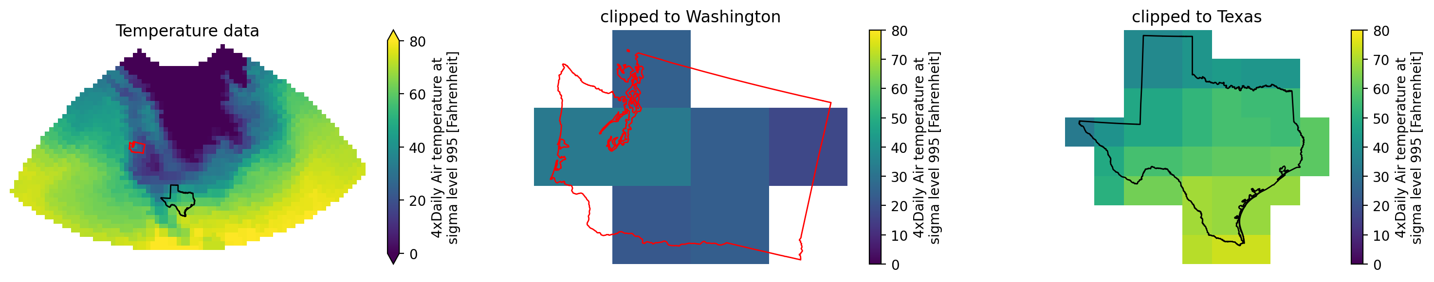
By the way, what does all_touched=True do in the .rio.clip() call?
Reading and writing files#
Xarray supports many disk formats. Below is a small example using netCDF. For more see the documentation
# write to netCDF
ds.to_netcdf("my-example-dataset.nc")
Note
To avoid the SerializationWarning you can assign a _FillValue for any NaNs in ‘air’ array by adding the keyword argument encoding=dict(air=dict(_FillValue=-9999))
# read from disk
fromdisk = xr.open_dataset("my-example-dataset.nc")
fromdisk
<xarray.Dataset> Size: 31MB
Dimensions: (lat: 25, time: 2920, lon: 53)
Coordinates:
* lat (lat) float32 100B 75.0 72.5 70.0 67.5 ... 22.5 20.0 17.5 15.0
* lon (lon) float32 212B 200.0 202.5 205.0 ... 325.0 327.5 330.0
* time (time) datetime64[ns] 23kB 2013-01-01 ... 2014-12-31T18:00:00
Data variables:
air (time, lat, lon) float64 31MB ...
spatial_ref int64 8B ...
Attributes:
Conventions: COARDS
title: 4x daily NMC reanalysis (1948)
description: Data is from NMC initialized reanalysis\n(4x/day). These a...
platform: Model
references: http://www.esrl.noaa.gov/psd/data/gridded/data.ncep.reanaly...# check that the two are identical
ds.identical(fromdisk)
False
Tip
A common use case to read datasets that are a collection of many netCDF files. See the documentation for how to handle that.
Finally to read other file formats, you might find yourself reading in the data using a different library and then creating a DataArray(docs, tutorial) from scratch. For example, you might use h5py to open an HDF5 file and then create a Dataset from that.
For MATLAB files you might use scipy.io.loadmat or h5py depending on the version of MATLAB file you’re opening and then construct a Dataset.
The scientific python ecosystem#
Xarray ties in to the larger scientific python ecosystem and in turn many packages build on top of xarray. A long list of such packages is here: https://docs.xarray.dev/en/stable/related-projects.html.
Now we will demonstrate some cool features.
Pandas: tabular data structures#
You can easily convert between xarray and pandas structures. This allows you to conveniently use the extensive pandas ecosystem of packages (like seaborn) for your work.
# convert to pandas dataframe
df = ds.isel(time=slice(10)).to_dataframe()
df
| air | spatial_ref | |||
|---|---|---|---|---|
| lat | time | lon | ||
| 75.0 | 2013-01-01 00:00:00 | 200.0 | -25.510 | 0 |
| 202.5 | -23.170 | 0 | ||
| 205.0 | -21.370 | 0 | ||
| 207.5 | -20.470 | 0 | ||
| 210.0 | -20.290 | 0 | ||
| ... | ... | ... | ... | ... |
| 15.0 | 2013-01-03 06:00:00 | 320.0 | 74.930 | 0 |
| 322.5 | 75.452 | 0 | ||
| 325.0 | 74.750 | 0 | ||
| 327.5 | 74.552 | 0 | ||
| 330.0 | 75.110 | 0 |
13250 rows × 2 columns
# convert dataframe to xarray
df.to_xarray()
<xarray.Dataset> Size: 212kB
Dimensions: (lat: 25, time: 10, lon: 53)
Coordinates:
* lat (lat) float32 100B 75.0 72.5 70.0 67.5 ... 22.5 20.0 17.5 15.0
* time (time) datetime64[ns] 80B 2013-01-01 ... 2013-01-03T06:00:00
* lon (lon) float32 212B 200.0 202.5 205.0 ... 325.0 327.5 330.0
Data variables:
air (lat, time, lon) float64 106kB -25.51 -23.17 ... 74.55 75.11
spatial_ref (lat, time, lon) int64 106kB 0 0 0 0 0 0 0 0 ... 0 0 0 0 0 0 0Alternative array types#
This notebook has focused on Numpy arrays. Xarray can wrap other array types! For example:
 distributed parallel arrays & Xarray user guide on Dask
![]() pydata/sparse : sparse arrays
pydata/sparse : sparse arrays
![]() pint : unit-aware arrays & pint-xarray
pint : unit-aware arrays & pint-xarray
Dask#
Dask cuts up NumPy arrays into blocks and parallelizes your analysis code across these blocks

# demonstrate dask dataset
dasky = xr.tutorial.open_dataset(
"air_temperature",
chunks={"time": 10}, # 10 time steps in each block
)
dasky.air
<xarray.DataArray 'air' (time: 2920, lat: 25, lon: 53)> Size: 31MB
dask.array<chunksize=(10, 25, 53), meta=np.ndarray>
Coordinates:
* lat (lat) float32 100B 75.0 72.5 70.0 67.5 65.0 ... 22.5 20.0 17.5 15.0
* lon (lon) float32 212B 200.0 202.5 205.0 207.5 ... 325.0 327.5 330.0
* time (time) datetime64[ns] 23kB 2013-01-01 ... 2014-12-31T18:00:00
Attributes:
long_name: 4xDaily Air temperature at sigma level 995
units: degK
precision: 2
GRIB_id: 11
GRIB_name: TMP
var_desc: Air temperature
dataset: NMC Reanalysis
level_desc: Surface
statistic: Individual Obs
parent_stat: Other
actual_range: [185.16 322.1 ]All computations with dask-backed xarray objects are lazy, allowing you to build up a complicated chain of analysis steps quickly
# demonstrate lazy mean
dasky.air.mean("lat")
<xarray.DataArray 'air' (time: 2920, lon: 53)> Size: 1MB
dask.array<chunksize=(10, 53), meta=np.ndarray>
Coordinates:
* lon (lon) float32 212B 200.0 202.5 205.0 207.5 ... 325.0 327.5 330.0
* time (time) datetime64[ns] 23kB 2013-01-01 ... 2014-12-31T18:00:00
Attributes:
long_name: 4xDaily Air temperature at sigma level 995
units: degK
precision: 2
GRIB_id: 11
GRIB_name: TMP
var_desc: Air temperature
dataset: NMC Reanalysis
level_desc: Surface
statistic: Individual Obs
parent_stat: Other
actual_range: [185.16 322.1 ]To get concrete values, call .compute or .load
# "compute" the mean
dasky.air.mean("lat").compute()
<xarray.DataArray 'air' (time: 2920, lon: 53)> Size: 1MB
279.4 279.7 279.7 279.7 280.0 279.9 ... 277.4 278.3 278.9 279.4 280.0 280.5
Coordinates:
* lon (lon) float32 212B 200.0 202.5 205.0 207.5 ... 325.0 327.5 330.0
* time (time) datetime64[ns] 23kB 2013-01-01 ... 2014-12-31T18:00:00
Attributes:
long_name: 4xDaily Air temperature at sigma level 995
units: degK
precision: 2
GRIB_id: 11
GRIB_name: TMP
var_desc: Air temperature
dataset: NMC Reanalysis
level_desc: Surface
statistic: Individual Obs
parent_stat: Other
actual_range: [185.16 322.1 ]# import hvplot.xarray
# ds.air.hvplot(groupby="time", clim=(270, 300), widget_location='bottom')
Other cool packages#
hvplot : quickly generate interactive plots from your data
xgcm : grid-aware operations with xarray objects
xrft : fourier transforms with xarray
xclim : calculating climate indices with xarray objects
intake-xarray : forget about file paths
rioxarray : raster files and xarray
xesmf : regrid using ESMF
MetPy : tools for working with weather data
Check the Xarray Ecosystem page and this tutorial for even more packages and demonstrations.
Next#
Read the tutorial material and user guide
See the description of common terms used in the xarray documentation:
Answers to common questions on “how to do X” with Xarray are here
Ryan Abernathey has a book on data analysis with a chapter on Xarray
Project Pythia has foundational and more advanced material on Xarray. Pythia also aggregates other Python learning resources.
The Xarray Github Discussions and Pangeo Discourse are good places to ask questions.
Tell your friends! Tweet!
Welcome!#
Xarray is an open-source project and gladly welcomes all kinds of contributions. This could include reporting bugs, discussing new enhancements, contributing code, helping answer user questions, contributing documentation (even small edits like fixing spelling mistakes or rewording to make the text clearer). Welcome!