Lab 08 assignment (20 pts)

Lab 08 assignment (20 pts)#

UW Geospatial Data Analysis
CEE467/CEWA567
David Shean, Eric Gagliano, Quinn Brencher

Introduction#

Objectives#

Explore spatial and temporal relationships of time series data
Work with Pandas Timestamp and Python DateTime objects
Handle data gaps effectively
Determine correlation of time-series records
Investigate and interpret spatial and temporal autocorrelation
Try out some interpolation routines to create continuous gridded values from sparse points
Visualize recent snow accumulation in your region
Learn about the SNOTEL network and explore some fundamental concepts and metrics for snow science

Instructions#

For each question or task below, write some code in the empty cell and execute to preserve your output
If you are in the graduate section of the class, please complete the challenge questions
Work together, consult resources we’ve discussed, post on slack!

Part 0: Imports and filenames#

First, let’s import the libraries we’ll need. Make sure to shut down any other kernels you have running!#

import os
from datetime import datetime
import numpy as np
import matplotlib.pyplot as plt
import pandas as pd
import geopandas as gpd
from shapely.geometry import Point
import folium
import contextily as ctx
import scipy.stats
import scipy.interpolate
import tqdm
from pathlib import Path
import xarray as xr
import skgstat as skg
import seaborn as sns
import pysal
from pysal.explore import esda
from pysal.lib import weights
from splot.esda import moran_scatterplot
from sklearn.preprocessing import StandardScaler
from sklearn.decomposition import PCA
from matplotlib_scalebar.scalebar import ScaleBar

/home/eric/miniconda3/envs/uwgda2025/lib/python3.12/site-packages/spaghetti/network.py:41: FutureWarning: The next major release of pysal/spaghetti (2.0.0) will drop support for all ``libpysal.cg`` geometries. This change is a first step in refactoring ``spaghetti`` that is expected to result in dramatically reduced runtimes for network instantiation and operations. Users currently requiring network and point pattern input as ``libpysal.cg`` geometries should prepare for this simply by converting to ``shapely`` geometries.
  warnings.warn(dep_msg, FutureWarning, stacklevel=1)

snotel_data_dir = f'{Path.home()}/gda_demo_data/snotel_data'

!ls -lh {snotel_data_dir}

total 1.1G
-rw-r--r-- 1 eric eric 1.1G Feb 27 19:10 snotel_data.nc
-rw-r--r-- 1 eric eric 456K Feb 27 19:09 snotel_stations.geojson

Part 1: Explore the SNOTEL sites (4 pts)#

Load SNOTEL sites geojson#

all_stations_gdf = gpd.read_file(f'{snotel_data_dir}/snotel_stations.geojson').set_index('code')
all_stations_gdf

	name	network	elevation_m	latitude	longitude	state	HUC	mgrs	mountainRange	beginDate	endDate	csvData	geometry
code
301_CA_SNTL	Adin Mtn	SNOTEL	1886.712036	41.235828	-120.791924	California	180200021403	10TFL	Great Basin Ranges	1983-10-01	2025-02-27	True	POINT (-120.79192 41.23583)
907_UT_SNTL	Agua Canyon	SNOTEL	2712.719971	37.522171	-112.271179	Utah	160300020301	12SUG	Colorado Plateau	1994-10-01	2025-02-27	True	POINT (-112.27118 37.52217)
916_MT_SNTL	Albro Lake	SNOTEL	2529.840088	45.597229	-111.959023	Montana	100200050701	12TVR	Central Montana Rocky Mountains	1996-09-01	2025-02-27	True	POINT (-111.95902 45.59723)
1267_AK_SNTL	Alexander Lake	SNOTEL	48.768002	61.749668	-150.889664	Alaska	190205051106	05VPJ	None	2014-08-28	2025-02-27	True	POINT (-150.88966 61.74967)
908_WA_SNTL	Alpine Meadows	SNOTEL	1066.800049	47.779572	-121.698471	Washington	171100100501	10TET	Cascade Range	1994-09-01	2025-02-27	True	POINT (-121.69847 47.77957)
...	...	...	...	...	...	...	...	...	...	...	...	...	...
SLT	Slate Creek	CCSS	1737.360000	41.043980	-122.480103	California	180200050304	10TEL	Klamath Mountains	2004-10-01	2025-02-27	True	POINT (-122.4801 41.04398)
SLI	Slide Canyon	CCSS	2804.160000	38.091234	-119.431881	California	180400090501	11SKC	Sierra Nevada	2005-10-01	2025-02-27	True	POINT (-119.43188 38.09123)
SLK	South Lake	CCSS	2926.080000	37.175903	-118.562660	California	180901020601	11SLB	Sierra Nevada	2004-10-01	2025-02-27	True	POINT (-118.56266 37.1759)
STL	State Lakes	CCSS	3169.920000	36.926483	-118.573250	California	180300100305	11SLA	Sierra Nevada	2018-11-01	2025-02-27	True	POINT (-118.57325 36.92648)
TMR	Tamarack Summit	CCSS	2301.240000	37.163750	-119.200531	California	180400060903	11SLB	Sierra Nevada	2011-01-01	2025-02-27	True	POINT (-119.20053 37.16375)

969 rows × 13 columns

Let’s quickly visualize with `.explore()`#

When you’re done, comment the following cell out, and rerun the cell to clear the plot, then save the notebook

#all_stations_gdf.drop(columns=['beginDate','endDate']).explore(column='elevation_m', cmap='inferno')

Written response: Where are station locations the most dense? Are there any areas you think are undersampled?#

STUDENT WRITTEN RESPONSE HERE

Load in state data, filter out Alaska stations, and reproject#

Can use the same Albers Equal Area projection from previous labs, or recompute based on bounds and center of SNOTEL sites

states_url = 'http://eric.clst.org/assets/wiki/uploads/Stuff/gz_2010_us_040_00_5m.json'
states_gdf = gpd.read_file(states_url)

Remove stations in Alaska from the `all_stations_gdf`#

You could use the .clip() function, or maybe even easier you can use the all_stations_gdf name column

# STUDENT CODE HERE

	name	network	elevation_m	latitude	longitude	state	HUC	mgrs	mountainRange	beginDate	endDate	csvData	geometry
code
755_NM_SNTL	Signal Peak	SNOTEL	2548.127930	32.924011	-108.145378	New Mexico	150400010803	12SYB	Southwest Basins and Ranges	1978-10-01	2025-02-27	True	POINT (-108.14538 32.92401)
1048_NM_SNTL	Mcknight Cabin	SNOTEL	2816.352051	33.008121	-107.869751	New Mexico	130302020103	13SBS	Southwest Basins and Ranges	2003-09-25	2025-02-27	True	POINT (-107.86975 33.00812)
595_NM_SNTL	Lookout Mountain	SNOTEL	2590.800049	33.360271	-107.831223	New Mexico	150400010402	13SBS	Southwest Basins and Ranges	1978-10-01	2025-02-27	True	POINT (-107.83122 33.36027)
757_NM_SNTL	Silver Creek Divide	SNOTEL	2743.199951	33.371059	-108.706177	New Mexico	150400040605	12SYB	Southwest Basins and Ranges	1978-10-01	2025-02-27	True	POINT (-108.70618 33.37106)
486_NM_SNTL	Frisco Divide	SNOTEL	2438.399902	33.736462	-108.945023	New Mexico	150400040303	12SXC	Colorado Plateau	1971-10-01	2025-02-27	True	POINT (-108.94502 33.73646)
...	...	...	...	...	...	...	...	...	...	...	...	...	...
1159_WA_SNTL	Gold Axe Camp	SNOTEL	1633.728027	48.951599	-118.986397	Washington	170200021204	11ULQ	Columbia Mountains	2010-10-01	2025-02-27	True	POINT (-118.9864 48.9516)
1107_WA_SNTL	Buckinghorse	SNOTEL	1484.375977	47.708599	-123.457474	Washington	171100200501	10TDT	Olympic Mountains	2008-06-19	2025-02-27	True	POINT (-123.45747 47.7086)
648_WA_SNTL	Mount Crag	SNOTEL	1207.008057	47.763699	-123.026001	Washington	171100180601	10TDT	Olympic Mountains	1989-10-01	2025-02-27	True	POINT (-123.026 47.7637)
943_WA_SNTL	Dungeness	SNOTEL	1222.248047	47.872238	-123.078796	Washington	171100200301	10TDU	Olympic Mountains	1998-10-01	2025-02-27	True	POINT (-123.0788 47.87224)
974_WA_SNTL	Waterhole	SNOTEL	1527.047974	47.944851	-123.425941	Washington	171100200506	10TDU	Olympic Mountains	1999-09-30	2025-02-27	True	POINT (-123.42594 47.94485)

926 rows × 13 columns

Calculate the convex hull of the remaining stations. Create an Albers Equal Area projection string, using the center of the convex hull as the center lat and lon, and the min and max latitude bound of the convex hull as the standard parallels.#

Hint: We did something similar in lab 03!

# STUDENT CODE HERE

# STUDENT CODE HERE

'+proj=aea +lat_1=32.92 +lat_2=48.98 +lat_0=41.66 +lon_0=-113.61'

Reproject our stations and states geodataframes to this new projection, and then create a plot of SNOTEL station locations and elevations overlaid on the states geometries and a basemap.#

all_stations_gdf = all_stations_gdf.to_crs(proj_str_aea)
states_gdf = states_gdf.to_crs(proj_str_aea)

# STUDENT CODE HERE

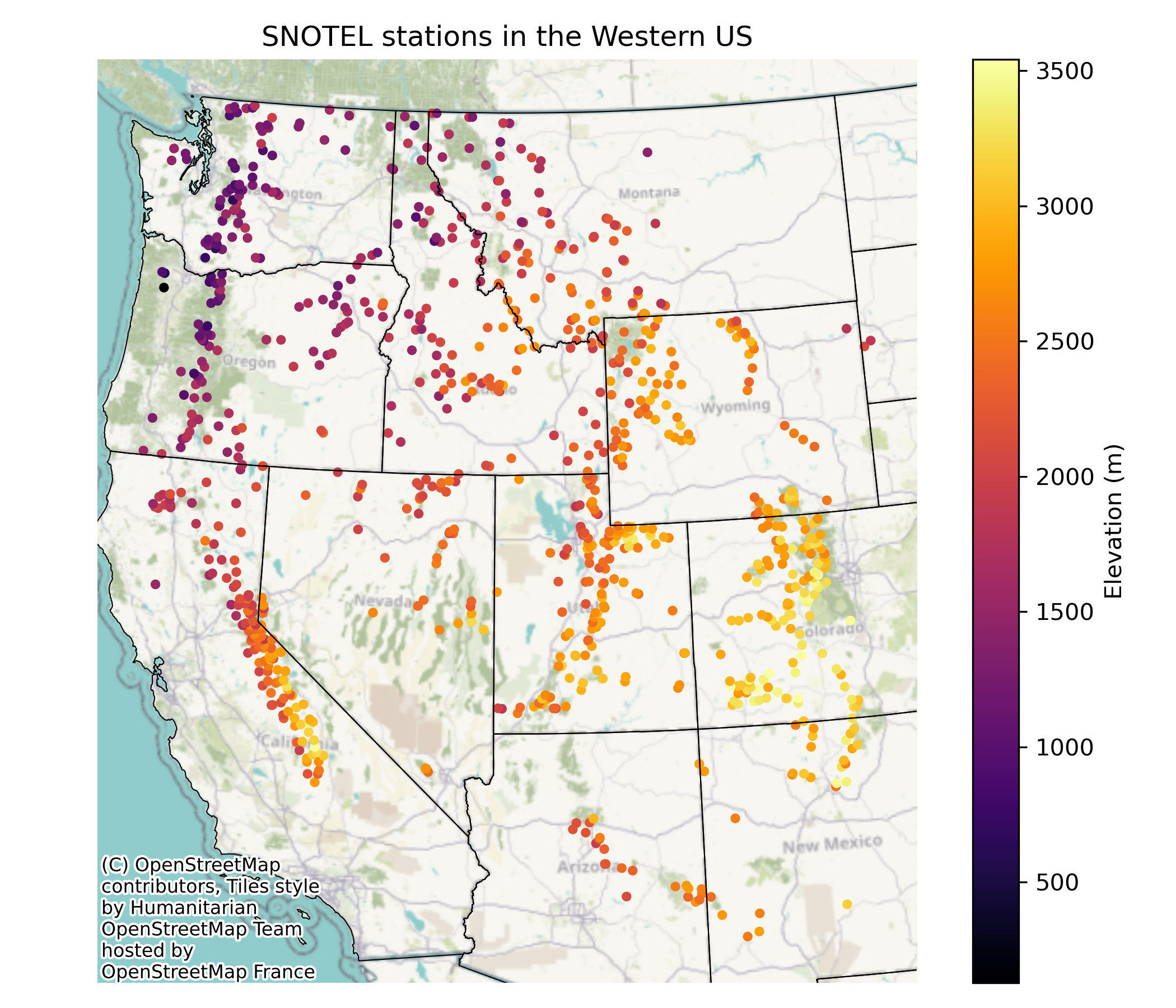
Print the station name, code, latitude, longitude, state, and elevation of the highest and lowest stations#

# STUDENT CODE HERE

Create `wa_stations_gdf`, a geodataframe of just the stations in Washington. Create a figure with three plots: a map of all of the stations (still excluding Alaska), a map of the Washington stations, and then one plot with their respective elevation histograms.#

To get the layout similar to the example output, maybe give subplot_mosaic a try!

wa_stations_gdf = all_stations_gdf[all_stations_gdf['state']=='Washington']
wa_stations_gdf

	name	network	elevation_m	latitude	longitude	state	HUC	mgrs	mountainRange	beginDate	endDate	csvData	geometry
code
1231_WA_SNTL	Satus Pass	SNOTEL	1207.008057	45.987968	-120.677338	Washington	170701060301	10TFR	Columbia Plateau	2012-08-23 00:00:00	2025-02-27	True	POINT (-543481.686 506823.621)
1129_WA_SNTL	Indian Rock	SNOTEL	1633.728027	45.990768	-120.807671	Washington	170701060301	10TFR	Columbia Plateau	2008-10-01 00:00:00	2025-02-27	True	POINT (-553456.824 507945.588)
804_WA_SNTL	Surprise Lakes	SNOTEL	1307.592041	46.094971	-121.763451	Washington	170800020107	10TES	Cascade Range	1978-10-01 00:00:00	2025-02-27	True	POINT (-625678.614 525941.149)
1109_WA_SNTL	Calamity	SNOTEL	762.000000	45.903622	-122.216331	Washington	170800020603	10TER	Cascade Range	2008-08-21 13:00:00	2025-02-27	True	POINT (-662408.042 507935.784)
1104_WA_SNTL	Pepper Creek	SNOTEL	652.271973	46.102421	-121.955551	Washington	170800020111	10TES	Cascade Range	2007-08-15 00:00:00	2025-02-27	True	POINT (-640297.907 528148.262)
...	...	...	...	...	...	...	...	...	...	...	...	...	...
1159_WA_SNTL	Gold Axe Camp	SNOTEL	1633.728027	48.951599	-118.986397	Washington	170200021204	11ULQ	Columbia Mountains	2010-10-01 00:00:00	2025-02-27	True	POINT (-393507.081 827717.25)
1107_WA_SNTL	Buckinghorse	SNOTEL	1484.375977	47.708599	-123.457474	Washington	171100200501	10TDT	Olympic Mountains	2008-06-19 00:00:00	2025-02-27	True	POINT (-735115.743 718322.713)
648_WA_SNTL	Mount Crag	SNOTEL	1207.008057	47.763699	-123.026001	Washington	171100180601	10TDT	Olympic Mountains	1989-10-01 00:00:00	2025-02-27	True	POINT (-702377.025 720918.663)
943_WA_SNTL	Dungeness	SNOTEL	1222.248047	47.872238	-123.078796	Washington	171100200301	10TDU	Olympic Mountains	1998-10-01 00:00:00	2025-02-27	True	POINT (-705004.394 733374.132)
974_WA_SNTL	Waterhole	SNOTEL	1527.047974	47.944851	-123.425941	Washington	171100200506	10TDU	Olympic Mountains	1999-09-30 00:00:00	2025-02-27	True	POINT (-729848.2 744242.973)

74 rows × 13 columns

# STUDENT CODE HERE

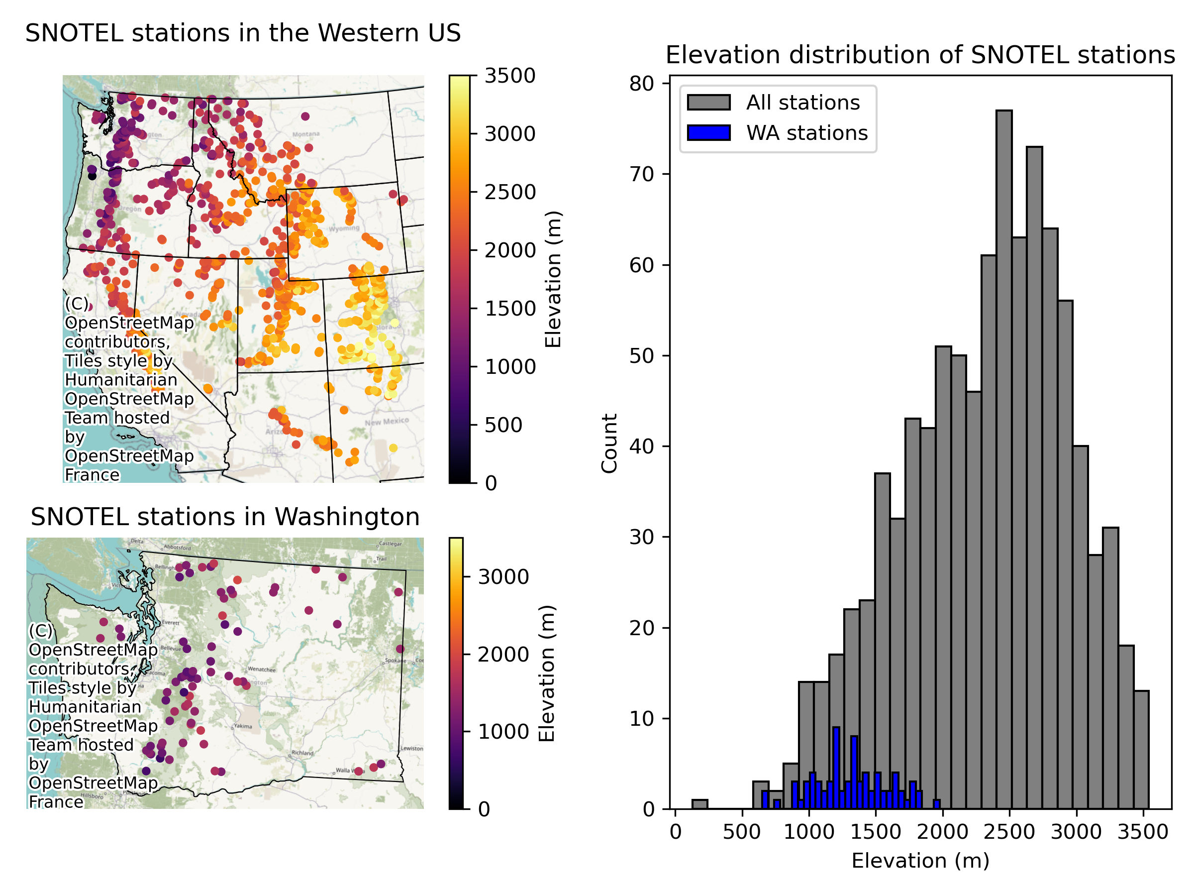
../../_images/snotel_stations_all_wa_comparison.png

Written response: Imagine using traditional statistical tests to answer each of the following questions. For each, comment on whether you think spatial autocorrelation is a concern and why. For traditional statistics, what assumptions are violated due to spatial autocorrelation?#

Based on the SNOTEL station data, is the average elevation in Washington different from the rest of the Contiguous US?
Are Washington’s SNOTEL station elevations representative of the broader SNOTEL network?

STUDENT WRITTEN RESPONSE HERE

Part 2: Single site time series analysis and temporal autocorrelation (5 pts)#

Here we’ll use the `.to_pandas()` function to turn our xarray dataset into a pandas dataframe#

paradise_snotel_df = paradise_snotel_ds.to_pandas()[['SNWD', 'TAVG','PRCPSA','WY','DOWY']]
paradise_snotel_df

	SNWD	TAVG	PRCPSA	WY	DOWY
time
1909-04-13	NaN	NaN	NaN	1909	195
1954-12-01	NaN	NaN	NaN	1955	62
1954-12-02	NaN	NaN	NaN	1955	63
1954-12-03	NaN	NaN	NaN	1955	64
1954-12-04	NaN	NaN	NaN	1955	65
...	...	...	...	...	...
2025-02-23	3.2512	1.8	0.0432	2025	146
2025-02-24	3.0734	1.3	0.0178	2025	147
2025-02-25	2.9718	-1.3	0.0432	2025	148
2025-02-26	NaN	-2.5	0.0025	2025	149
2025-02-27	3.3782	NaN	NaN	2025	150

24173 rows × 5 columns

Written response: You’ll notice we preserved the `WY` and `DOWY` columns. Read the water year wikipedia page. Why might water year and day of water year (DOWY) be useful for us when comparing snow hydrology data?#

STUDENT WRITTEN RESPONSE HERE

Plot snow depth vs day of water year, with colors representing average temperatures#

# STUDENT CODE HERE

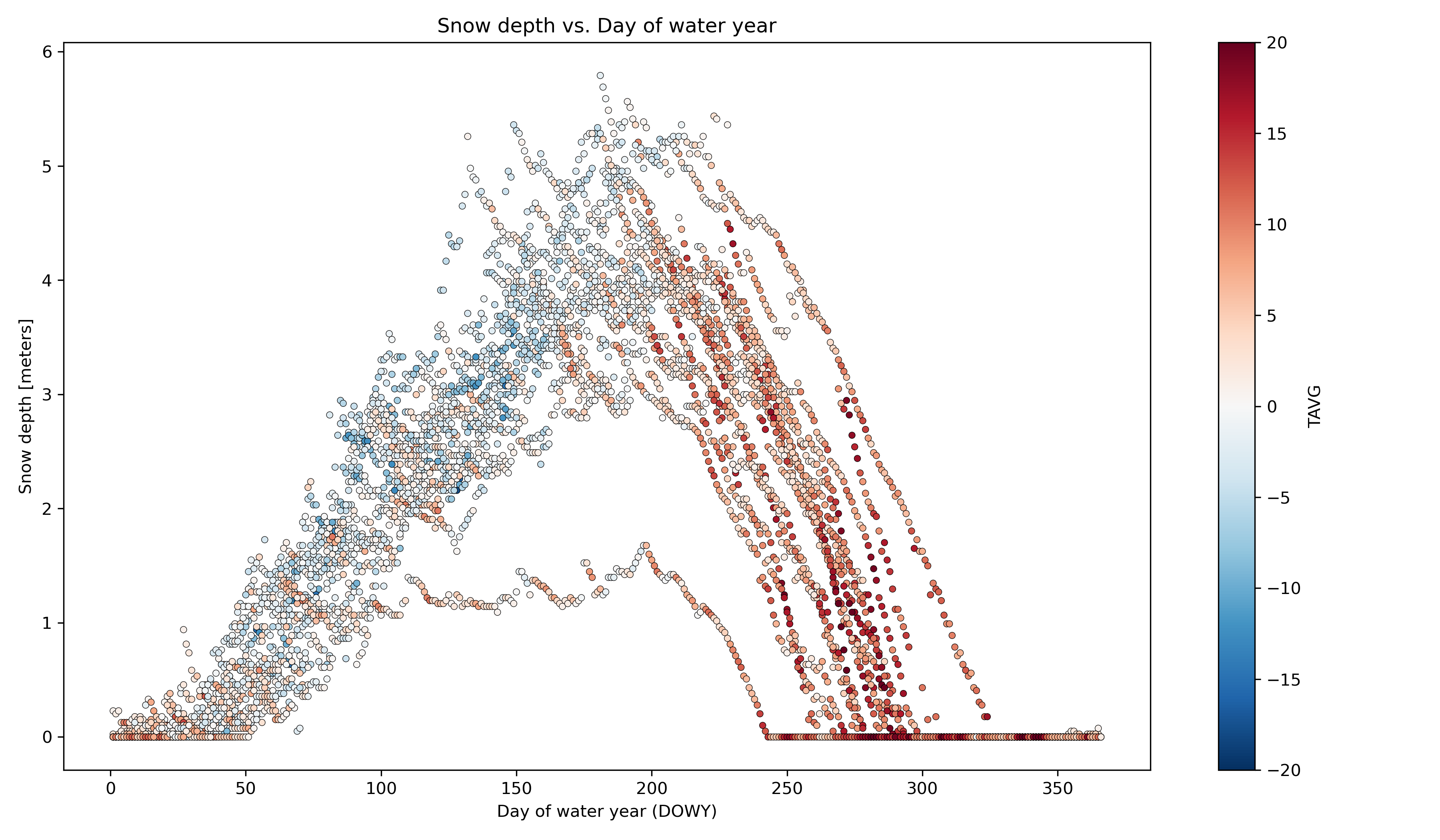
../../_images/paradise_snotel_snwd_vs_dowy_and_temp.png

Written response: Answer the following by inspecting the graph above. What is the approximate average maximum snow depth, and around what day does this occur? Around what average temperatures does it seem that snow depth decreases the fastest, and around what day does this usually occur? Around what day does snow usually disappear? Approximately what day did the snow disappear earliest? Latest? Please report the dates as both DOWY and calendar dates.#

STUDENT WRITTEN RESPONSE HERE

Compute statistics for each day of water year, using values from all years#

Seems like a Pandas groupby/agg might work here
Include min, max, mean, and median

stat_list = ['count','min','max','mean','std','median']

# STUDENT CODE HERE

	count	min	max	mean	std	median
DOWY
1	19	0.0	0.2286	0.013368	0.052444	0.0
2	19	0.0	0.2032	0.010695	0.046617	0.0
3	19	0.0	0.2286	0.013368	0.052444	0.0
4	19	0.0	0.1270	0.012032	0.032093	0.0
5	19	0.0	0.1270	0.012032	0.033192	0.0
...	...	...	...	...	...	...
362	19	0.0	0.0254	0.001337	0.005827	0.0
363	19	0.0	0.0254	0.001337	0.005827	0.0
364	19	0.0	0.0254	0.002674	0.008009	0.0
365	19	0.0	0.0762	0.005347	0.018117	0.0
366	5	0.0	0.0000	0.000000	0.000000	0.0

366 rows × 6 columns

What day of water year has the highest average snow depth, and what is that snow depth? What calendar day does this correspond to?#

Consider converting from DOWY to calendar date using caldate = pd.to_datetime('2021-09-30')+pd.to_timedelta(DOWY, unit='D')
And calmonthday = caldate.strftime('%B %d') to convert from pandas datetime to Month / day string

# STUDENT CODE HERE

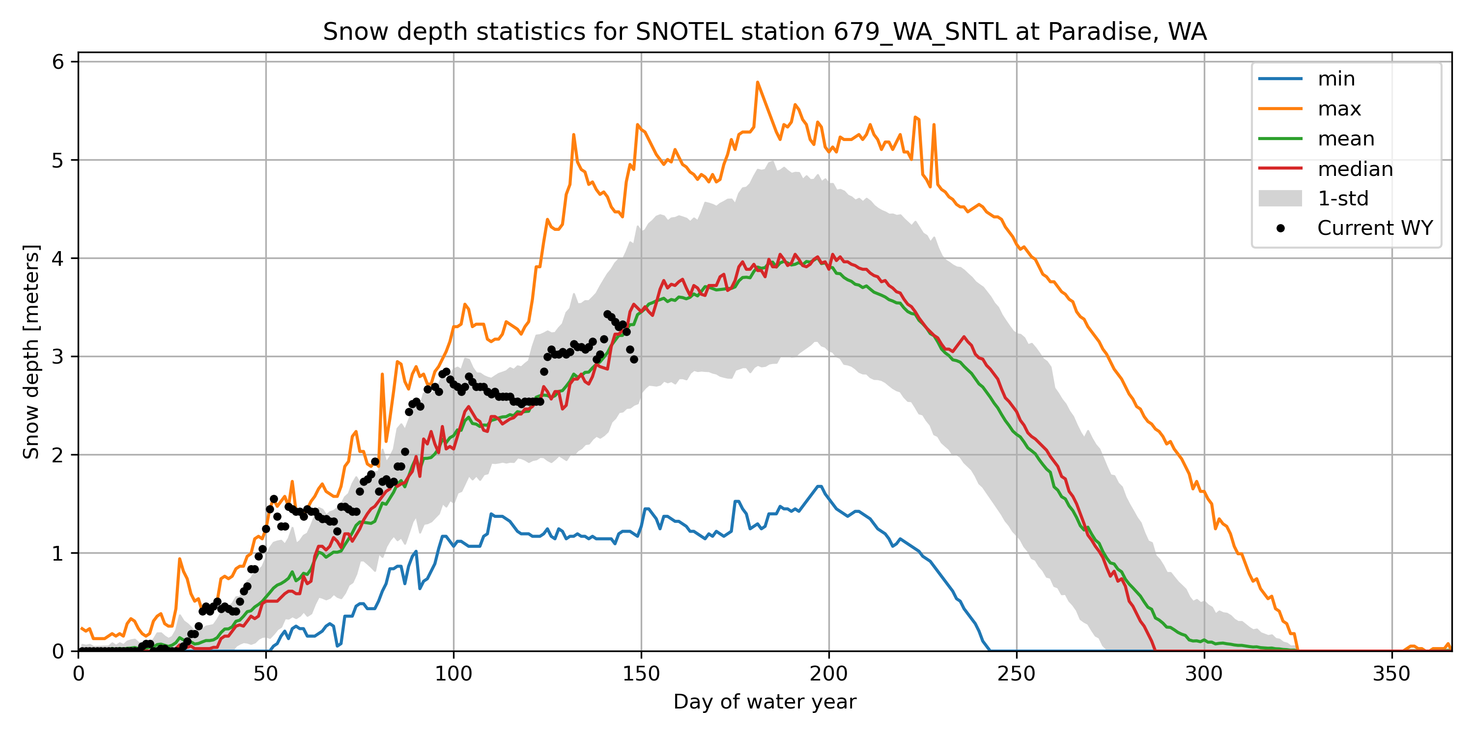
The day of highest average snow depth is DOWY 197, corresponding to a calendar date of April 15, with an average snow depth of 4.00 meters.

Create a plot of these aggregated dowy values, and add the current water year’s daily data as a scatter plot on top#

Your output independent variable (x-axis) should be day of water year (1-366), and dependent variable (y-axis) should be median value for that day of year, computed using aggregated values for all available years
You can add shaded regions for standard deviation using ax.fill_between

# STUDENT CODE HERE

../../_images/paradise_snotel_snwd_stats.png

For most recent snow depth value in the record, what is the percentage of “normal”#

This will be the snow depth from whenever you ran the download script
Normal can be defined by long-term median for the same dowy across all years at the site

# STUDENT CODE HERE

Current snow depth (February 25, 2025 / DOWY 148): 2.97 meters
Long-term median on DOWY 148: 3.53 meters
Percent of normal snow depth on DOWY 148: 84.17%

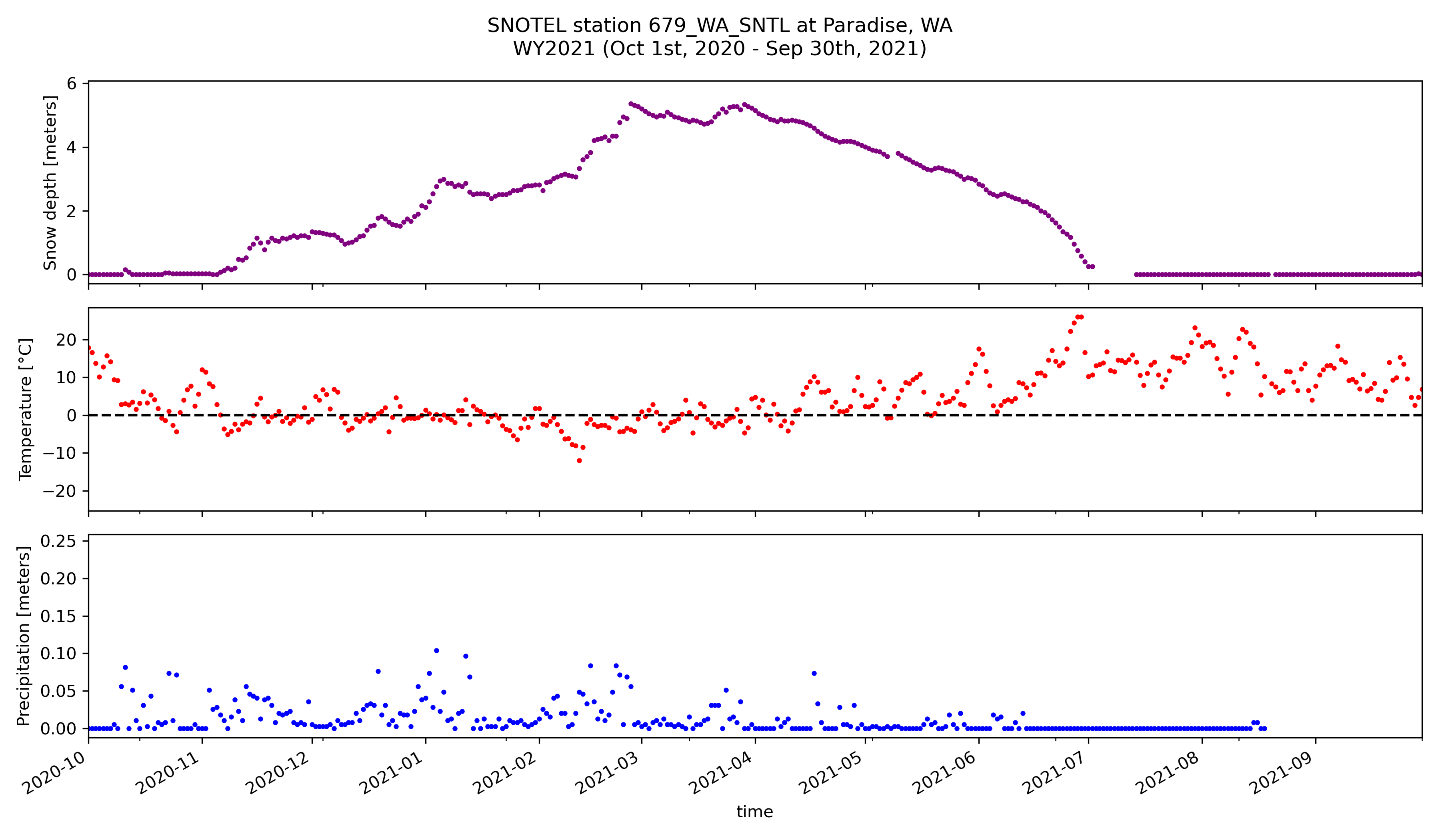
Now let’s view the data as time-series plots#

Create a figure to plot snow depth, temperature, and precipitation for water year 2021#

# STUDENT CODE HERE

../../_images/paradise_snotel_data_wy2021.png

Now we’ll calculate the temporal autocorrelation for WY 2021…#

autocorr_snwd = []
autocorr_tavg = []
autocorr_prcp = []
autocorr_lags = np.arange(1, 365)

paradise_snotel_wy2021_df = paradise_snotel_df.loc['2020-10-01':'2021-09-30']

for i in autocorr_lags:
    autocorr_snwd.append(paradise_snotel_wy2021_df['SNWD'].autocorr(lag=i))
    autocorr_tavg.append(paradise_snotel_wy2021_df['TAVG'].autocorr(lag=i))
    autocorr_prcp.append(paradise_snotel_wy2021_df['PRCPSA'].autocorr(lag=i))

/home/eric/miniconda3/envs/uwgda2025/lib/python3.12/site-packages/numpy/lib/_function_base_impl.py:2991: RuntimeWarning: Degrees of freedom <= 0 for slice
  c = cov(x, y, rowvar, dtype=dtype)

f,ax=plt.subplots(figsize=(12,7))
ax.plot(autocorr_lags, autocorr_snwd, marker='o', linestyle='-', color='purple', label='Snow depth',markersize=2)
ax.plot(autocorr_lags, autocorr_tavg, marker='o', linestyle='-', color='red', label='Temperature',markersize=2)
ax.plot(autocorr_lags, autocorr_prcp, marker='o', linestyle='-', color='blue', label='Precipitation',markersize=2)
ax.set_ylim([-1, 1])

ax.set_title('Autocorrelation of SNOTEL station data')
ax.set_xlabel('Lag (days)')
ax.set_ylabel('Autocorrelation')
ax.legend()

ax.axhline(0, color='k', linestyle='--')
ax.axhline(1, color='k', linestyle='--', alpha=0.5)
ax.axhline(-1, color='k', linestyle='--', alpha=0.5)
ax.grid(True)

f.tight_layout()

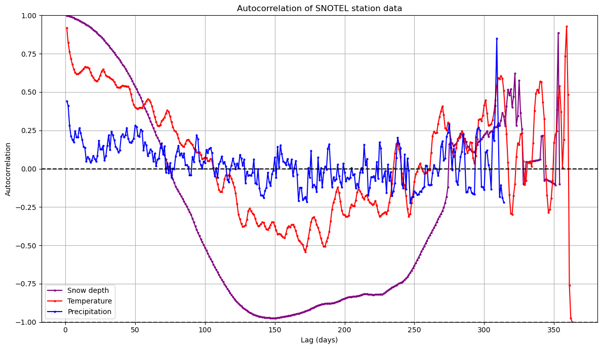
../../_images/6bcd75897422f3e313e941807ebacbf346f3ec340d8c7c1784e7ec93906b1524.png

Written response: Compare and contrast the autocorrelation patterns among these three variables. What distinctive features do you observe in each pattern, and what physical or environmental processes might explain these differences? Also, describe the significance of the relative magnitudes of the curves, as well as the significance of the autocorrelation values at a lag distance of one day.#

STUDENT WRITTEN RESPONSE HERE

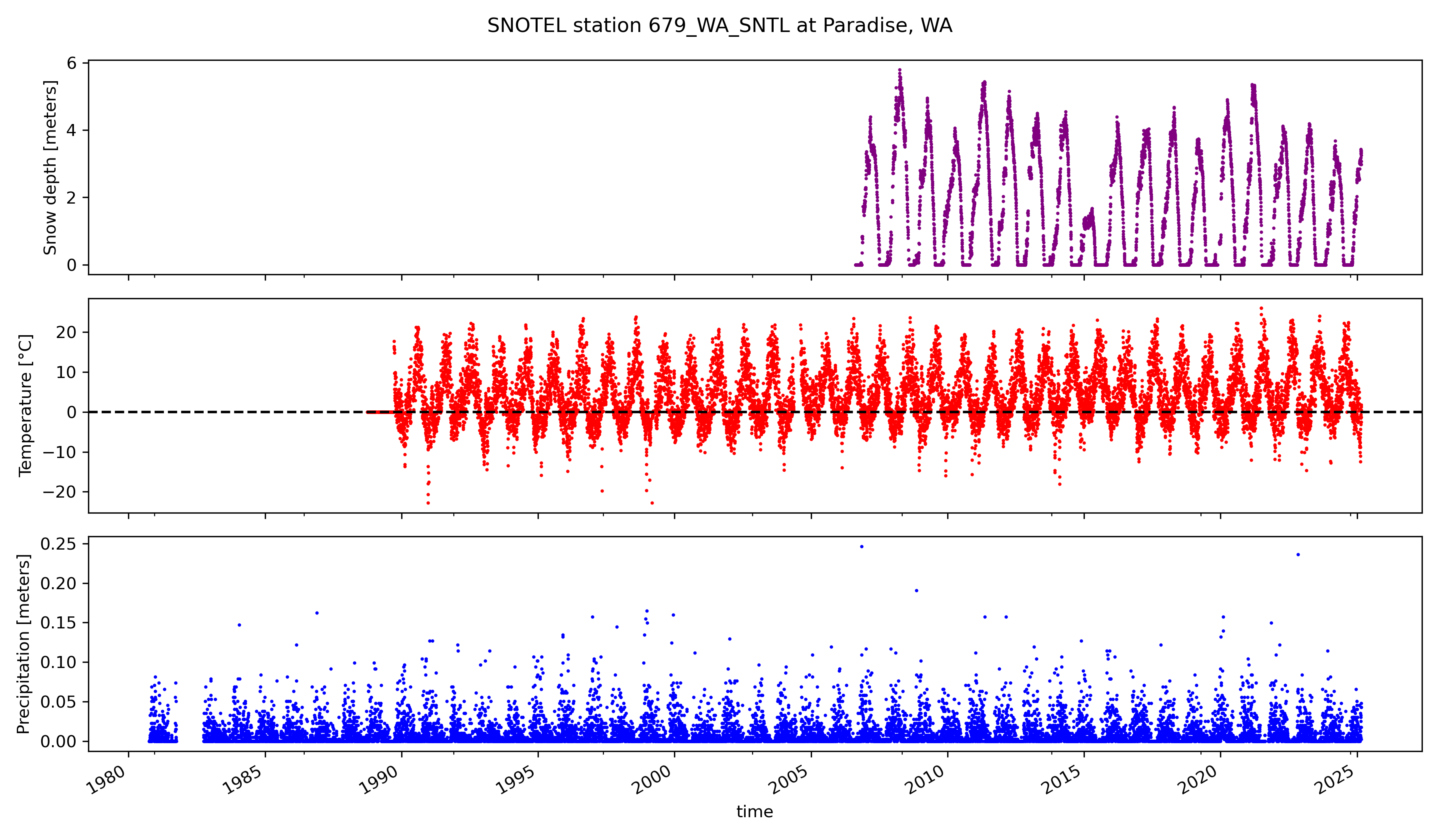
Now plot the same variables, but this time use the full time-series#

# STUDENT CODE HERE

../../_images/paradise_snotel_data_long.png

Now we’ll calculate the temporal autocorrelation for the entire time-series…#

autocorr_snwd = []
autocorr_tavg = []
autocorr_prcp = []
autocorr_lags = np.arange(1, 365*3)

for i in autocorr_lags:
    autocorr_snwd.append(paradise_snotel_df['SNWD'].autocorr(lag=i))
    autocorr_tavg.append(paradise_snotel_df['TAVG'].autocorr(lag=i))
    autocorr_prcp.append(paradise_snotel_df['PRCPSA'].autocorr(lag=i))

f,ax=plt.subplots(figsize=(12,7))
ax.plot(autocorr_lags, autocorr_snwd, marker='o', linestyle='-', color='purple', label='Snow depth', markersize=2)
ax.plot(autocorr_lags, autocorr_tavg, marker='o', linestyle='-', color='red', label='Temperature',markersize=2)
ax.plot(autocorr_lags, autocorr_prcp, marker='o', linestyle='-', color='blue', label='Precipitation',markersize=2)
ax.set_ylim([-1, 1])

ax.set_title('Autocorrelation of SNOTEL station data')
ax.set_xlabel('Lag (days)')
ax.set_ylabel('Autocorrelation')
ax.legend()

ax.axhline(0, color='k', linestyle='--')
ax.axhline(1, color='k', linestyle='--', alpha=0.5)
ax.axhline(-1, color='k', linestyle='--', alpha=0.5)
ax.grid(True)

f.tight_layout()

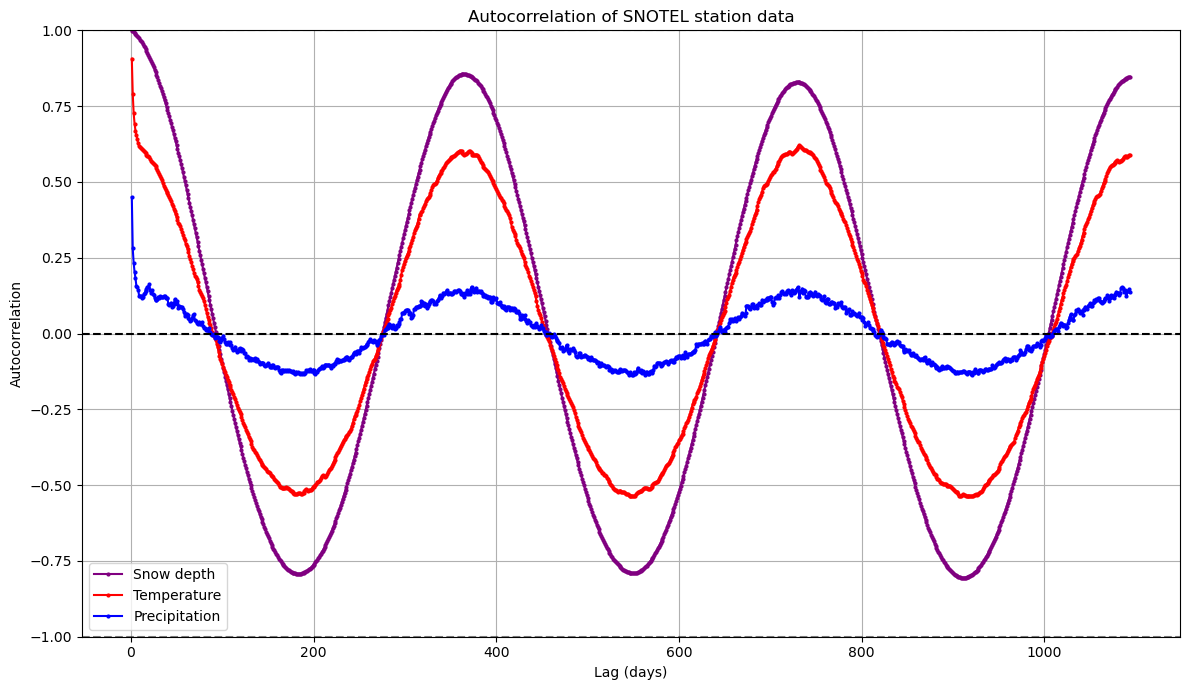
../../_images/ddb0f5458f071a9e0f419207d62be30f2dfafa01d041deabe4ae6ea570acd8c7.png

Written response: How might these autocorrelation patterns change at another SNOTEL site? Snow depth shows persistent positive autocorrelation over longer lags than precipitation. What implications does this have for the minimum timespan needed to characterize each process and the reliability of short-term vs. long-term forecasts?#

STUDENT WRITTEN RESPONSE HERE

What would the variogram for snow depth look like here??#

Technically, we shouldn’t use a variogram here because it violates an assumption of stationarity - check out a great explainer here
Stationarity is violated because the mean and variance are are not constant across all time points, and the covariance between points does not only depend on distance between them
- Think about how in the summer the mean and variability in snow depth are a lot lower than in the winter :)
But let’s plot it anyway to see what it would look like!

variogram_df = paradise_snotel_df["SNWD"].dropna()
delta_days = (pd.to_datetime(variogram_df.index)-pd.to_datetime(variogram_df.index.min())).days
variogram_df.index=delta_days

V = skg.Variogram(
    variogram_df.index.values,
    variogram_df.values,
    model="gaussian",
    maxlag=365*3,
    n_lags=50,
    use_nugget=True,
)
V.fit()

V.plot()

/home/eric/miniconda3/envs/uwgda2025/lib/python3.12/site-packages/skgstat/plotting/variogram_plot.py:123: UserWarning: FigureCanvasAgg is non-interactive, and thus cannot be shown
  fig.show()

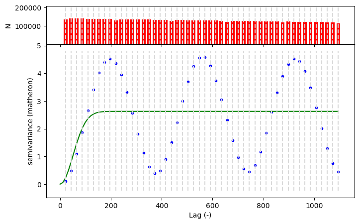
../../_images/391a6c80a0c2b7eab9b6fa3bebc0a97117d4d5df9072e8b54cc18d9994c54cfd.png

print("Snow depth variogram model parameters:")
print(f"Model type: {V.describe()['model']}")
print(f"Nugget: {V.describe()['nugget']:.4f}")
print(f"Sill: {V.describe()['sill']:.4f}")
print(f"Range indicates that spatial dependence extends to approximately: {V.describe()['effective_range']:.4f} days")

Snow depth variogram model parameters:
Model type: gaussian
Nugget: 0.0000
Sill: 2.6271
Range indicates that spatial dependence extends to approximately: 144.6148 days

Written response: Compare the shape of the variogram plot with the autocorrelation function for snow depth. What similarities or differences do you observe, and what mathematical relationship connects these two representations of dependency? From just the variogram alone, how might you tell that the stationarity assumption has been violated?#

Hint: Remember that the blue points show the true variances at different lag distances, and the green line is supposed to be fit to these points

STUDENT WRITTEN RESPONSE HERE

Part 3: Western U.S. time-series analysis and correlation (4 pts)#

Now let’s take a look at the full SNOTEL time-series for the Western US

Create `all_stations_snwd_df`, a pandas dataframe of snow depth at all stations, with each row representing a day, and each column representing a station#

all_stations_snwd_df = snotel_ds['SNWD'].to_pandas().T
all_stations_snwd_df

station	1135_UT_SNTL	448_MT_SNTL	TMR	872_WY_SNTL	773_CO_SNTL	MDW	1224_UT_SNTL	1109_WA_SNTL	1045_WY_SNTL	902_AZ_SNTL	...	310_AZ_SNTL	FOR	1207_NV_SNTL	349_MT_SNTL	368_UT_SNTL	644_WA_SNTL	327_CO_SNTL	417_NV_SNTL	544_WY_SNTL	915_ID_SNTL
time
1909-04-13	NaN	NaN	NaN	NaN	NaN	NaN	NaN	NaN	NaN	NaN	...	NaN	NaN	NaN	NaN	NaN	NaN	NaN	NaN	NaN	NaN
1954-12-01	NaN	NaN	NaN	NaN	NaN	NaN	NaN	NaN	NaN	NaN	...	NaN	NaN	NaN	NaN	NaN	NaN	NaN	NaN	NaN	NaN
1954-12-02	NaN	NaN	NaN	NaN	NaN	NaN	NaN	NaN	NaN	NaN	...	NaN	NaN	NaN	NaN	NaN	NaN	NaN	NaN	NaN	NaN
1954-12-03	NaN	NaN	NaN	NaN	NaN	NaN	NaN	NaN	NaN	NaN	...	NaN	NaN	NaN	NaN	NaN	NaN	NaN	NaN	NaN	NaN
1954-12-04	NaN	NaN	NaN	NaN	NaN	NaN	NaN	NaN	NaN	NaN	...	NaN	NaN	NaN	NaN	NaN	NaN	NaN	NaN	NaN	NaN
...	...	...	...	...	...	...	...	...	...	...	...	...	...	...	...	...	...	...	...	...	...
2025-02-23	0.5334	0.6858	0.4826	0.5588	0.8636	3.5306	1.2700	0.0	0.4064	0.0	...	0.0	NaN	0.7112	0.9144	1.1938	1.1176	1.1938	1.3716	1.9558	0.9144
2025-02-24	0.5080	0.7366	0.4572	0.5588	0.8636	3.4544	1.2192	0.0	0.3810	0.0	...	0.0	NaN	0.7112	0.9144	1.1684	1.1176	1.1938	1.3462	1.9304	0.9398
2025-02-25	0.4572	0.7366	0.4318	0.5334	0.8636	3.4036	1.1684	0.0	0.3556	0.0	...	0.0	NaN	0.6604	0.8890	1.1430	1.1430	1.1684	1.2954	1.9050	0.9398
2025-02-26	0.4572	0.7620	0.4318	0.5334	0.8636	3.3528	1.1430	0.0	0.3556	0.0	...	0.0	NaN	0.6604	0.9144	1.1176	1.1430	1.1684	1.2700	1.9050	0.9398
2025-02-27	0.4572	0.7620	0.4064	0.5334	0.9906	3.3020	1.1430	0.0	0.3556	0.0	...	0.0	NaN	0.6350	0.9144	1.1176	1.1430	1.1684	1.2700	1.8796	0.9398

24173 rows × 969 columns

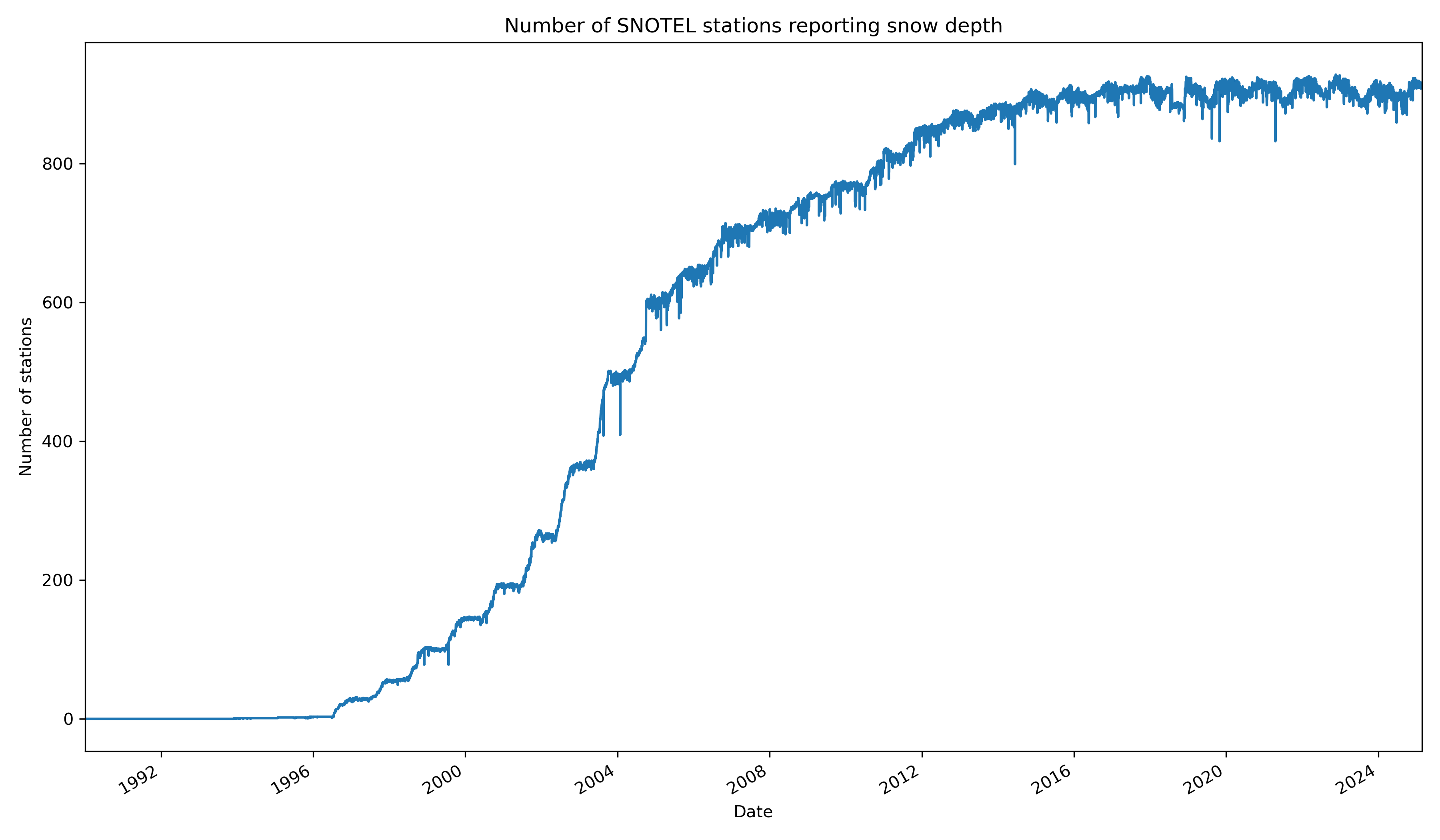
Create a plot of total operational stations vs time#

Limit your plot from January 1st, 1990 to February 24th, 2025

Hint: Remember the Pandas count function
- Make sure do the count over the right axis of the DataFrame
Hint: If you’re plotting a dataframe with a DatetimeIndex, you can set your xlim like… ax.set_xlim(['YYYY-MM-DD','YYYY-MM-DD'])

# STUDENT CODE HERE

../../_images/snotel_stations_reporting.png

Create a histogram of all snow depth values#

Use the Pandas stack function here, otherwise you will end up with histograms for each station
Consider using log scale, as you likely have a spike for days with 0 snow depth (several months of each year!)
Adjust the x axis limits to realistic bounds for snow depth, excluding some spurious data

# STUDENT CODE HERE

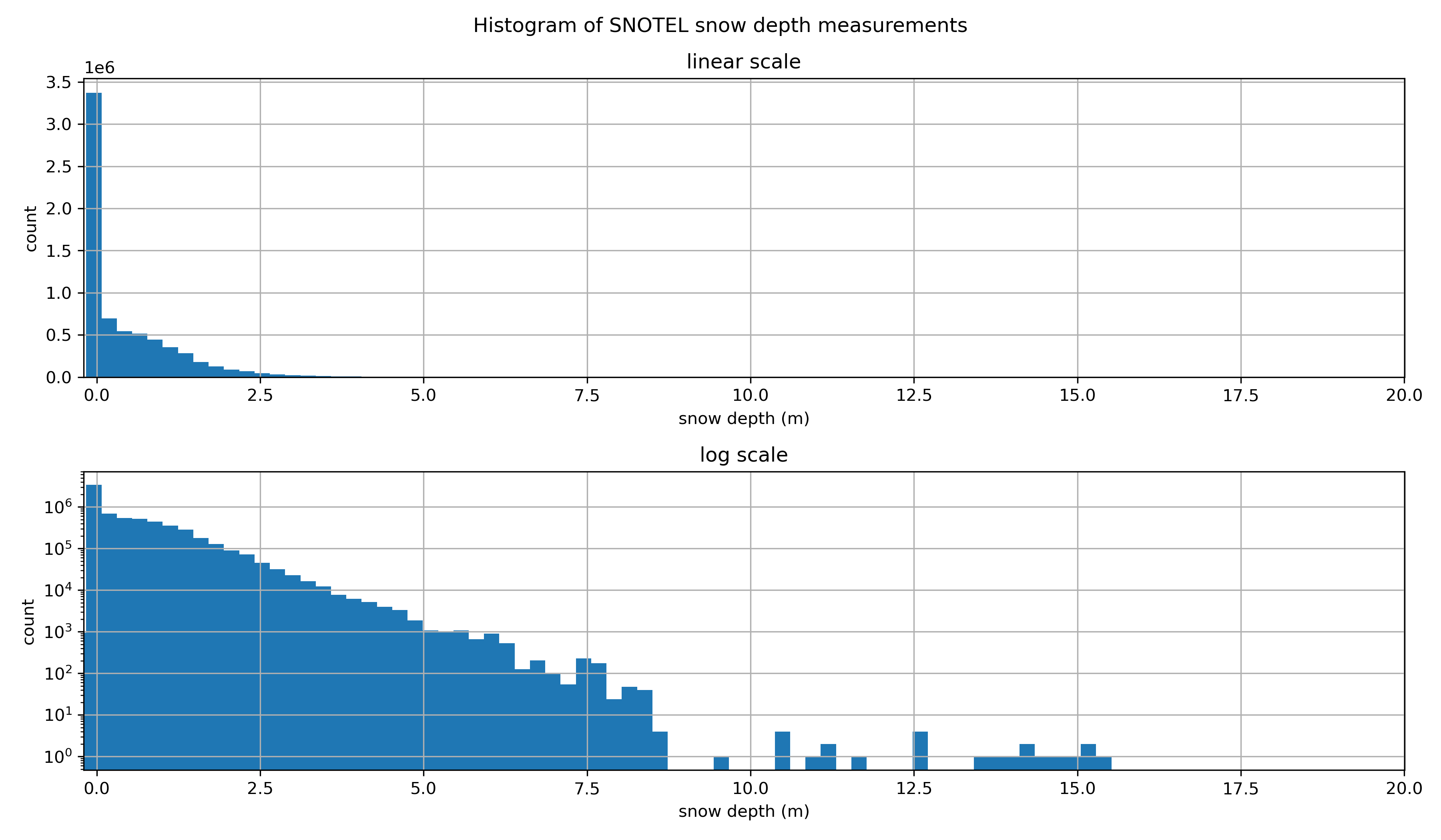
Hmmm, let’s filter out snow depth values less than one centimeter and greater than 10 meters. This will help with our aggregations later, as well as remove unlikely values.#

all_stations_snwd_df = all_stations_snwd_df.where((all_stations_snwd_df >= 0.01) & (all_stations_snwd_df <= 10.0))  # Filter out negative values and outliers
all_stations_snwd_df

station	1135_UT_SNTL	448_MT_SNTL	TMR	872_WY_SNTL	773_CO_SNTL	MDW	1224_UT_SNTL	1109_WA_SNTL	1045_WY_SNTL	902_AZ_SNTL	...	310_AZ_SNTL	FOR	1207_NV_SNTL	349_MT_SNTL	368_UT_SNTL	644_WA_SNTL	327_CO_SNTL	417_NV_SNTL	544_WY_SNTL	915_ID_SNTL
time
1909-04-13	NaN	NaN	NaN	NaN	NaN	NaN	NaN	NaN	NaN	NaN	...	NaN	NaN	NaN	NaN	NaN	NaN	NaN	NaN	NaN	NaN
1954-12-01	NaN	NaN	NaN	NaN	NaN	NaN	NaN	NaN	NaN	NaN	...	NaN	NaN	NaN	NaN	NaN	NaN	NaN	NaN	NaN	NaN
1954-12-02	NaN	NaN	NaN	NaN	NaN	NaN	NaN	NaN	NaN	NaN	...	NaN	NaN	NaN	NaN	NaN	NaN	NaN	NaN	NaN	NaN
1954-12-03	NaN	NaN	NaN	NaN	NaN	NaN	NaN	NaN	NaN	NaN	...	NaN	NaN	NaN	NaN	NaN	NaN	NaN	NaN	NaN	NaN
1954-12-04	NaN	NaN	NaN	NaN	NaN	NaN	NaN	NaN	NaN	NaN	...	NaN	NaN	NaN	NaN	NaN	NaN	NaN	NaN	NaN	NaN
...	...	...	...	...	...	...	...	...	...	...	...	...	...	...	...	...	...	...	...	...	...
2025-02-23	0.5334	0.6858	0.4826	0.5588	0.8636	3.5306	1.2700	NaN	0.4064	NaN	...	NaN	NaN	0.7112	0.9144	1.1938	1.1176	1.1938	1.3716	1.9558	0.9144
2025-02-24	0.5080	0.7366	0.4572	0.5588	0.8636	3.4544	1.2192	NaN	0.3810	NaN	...	NaN	NaN	0.7112	0.9144	1.1684	1.1176	1.1938	1.3462	1.9304	0.9398
2025-02-25	0.4572	0.7366	0.4318	0.5334	0.8636	3.4036	1.1684	NaN	0.3556	NaN	...	NaN	NaN	0.6604	0.8890	1.1430	1.1430	1.1684	1.2954	1.9050	0.9398
2025-02-26	0.4572	0.7620	0.4318	0.5334	0.8636	3.3528	1.1430	NaN	0.3556	NaN	...	NaN	NaN	0.6604	0.9144	1.1176	1.1430	1.1684	1.2700	1.9050	0.9398
2025-02-27	0.4572	0.7620	0.4064	0.5334	0.9906	3.3020	1.1430	NaN	0.3556	NaN	...	NaN	NaN	0.6350	0.9144	1.1176	1.1430	1.1684	1.2700	1.8796	0.9398

24173 rows × 969 columns

Use the built-in `.describe()` function to determine look at some quick statistics. Which station has the highest mean snow depth? Which station has the greatest number of days with snow depth data?#

# STUDENT CODE HERE

station	1135_UT_SNTL	448_MT_SNTL	TMR	872_WY_SNTL	773_CO_SNTL	MDW	1224_UT_SNTL	1109_WA_SNTL	1045_WY_SNTL	902_AZ_SNTL	...	310_AZ_SNTL	FOR	1207_NV_SNTL	349_MT_SNTL	368_UT_SNTL	644_WA_SNTL	327_CO_SNTL	417_NV_SNTL	544_WY_SNTL	915_ID_SNTL
count	2570.000000	5801.000000	3859.000000	3950.000000	4949.000000	4021.000000	2729.000000	1402.000000	3968.000000	2159.000000	...	2600.000000	0.0	1879.000000	4923.000000	4991.000000	4080.000000	5290.000000	4778.000000	2260.000000	2968.000000
mean	0.350263	0.578521	0.528608	0.412072	0.817902	1.339466	0.991549	0.310018	0.342663	0.208953	...	0.373908	NaN	0.365887	0.563284	1.015669	0.671158	0.961167	0.860378	1.096830	0.568479
std	0.201622	0.320822	0.811378	0.272422	0.538385	1.431758	0.595782	0.251574	0.204886	0.192829	...	0.291448	NaN	0.279400	0.336501	0.584000	0.395396	0.581579	0.512492	0.626058	0.331571
min	0.025400	0.025400	0.025400	0.025400	0.025400	0.025400	0.025400	0.025400	0.025400	0.025400	...	0.025400	NaN	0.025400	0.025400	0.025400	0.025400	0.025400	0.025400	0.025400	0.025400
25%	0.203200	0.304800	0.025400	0.177800	0.330200	0.076200	0.482600	0.082550	0.177800	0.050800	...	0.127000	NaN	0.127000	0.279400	0.533400	0.355600	0.482600	0.457200	0.558800	0.279400
50%	0.355600	0.609600	0.076200	0.406400	0.812800	0.939800	1.016000	0.254000	0.355600	0.152400	...	0.355600	NaN	0.279400	0.558800	1.016000	0.635000	0.965200	0.863600	1.168400	0.584200
75%	0.508000	0.812800	0.685800	0.609600	1.219200	2.184400	1.371600	0.457200	0.482600	0.304800	...	0.533400	NaN	0.584200	0.812800	1.371600	0.965200	1.371600	1.219200	1.549400	0.812800
max	1.041400	1.422400	4.572000	1.422400	2.336800	7.010400	3.048000	1.143000	1.092200	1.193800	...	1.828800	NaN	1.244600	1.498600	2.692400	1.828800	2.971800	2.819400	2.819400	1.397000

8 rows × 969 columns

# STUDENT CODE HERE

The station with the highest average snow depth is LOS with an average snow depth of 3.93 meters.
The station with the greatest number of days with snow depth data is 347_MT_SNTL with 8098 days.

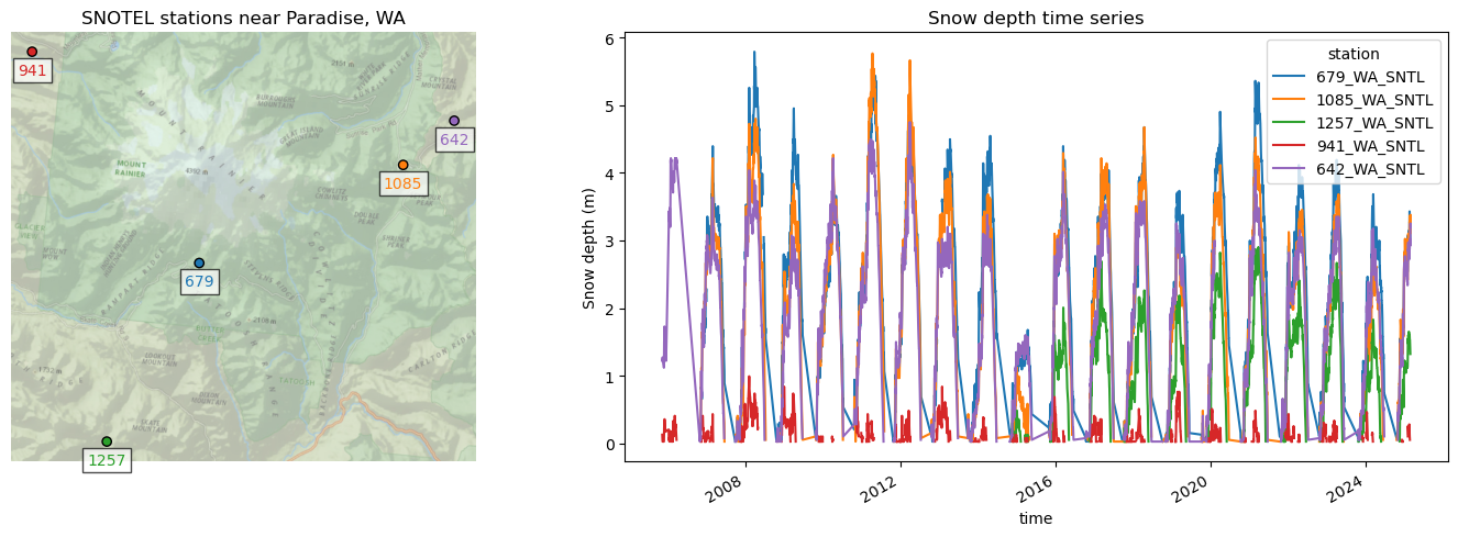
Temporal correlation of snow depth for nearby stations#

Can use Paradise (‘SNOTEL:679_WA_SNTL’) and nearby station identified on the labeled folium plot above
Plot the time series for all stations
Can also use dropna here, but careful about methodology (any vs all, vs thresh)

#Paradise and nearby sites
site1 = '679_WA_SNTL'
site2 = '1085_WA_SNTL'
site3 = '1257_WA_SNTL'
site4 = '941_WA_SNTL'
site5 = '642_WA_SNTL'

site_list = [site1,site2,site3,site4,site5]
color_list = ['C%i' % i for i in range(len(site_list))]

nearby_gdf = all_stations_gdf.loc[site_list]
nearby_gdf

	name	network	elevation_m	latitude	longitude	state	HUC	mgrs	mountainRange	beginDate	endDate	csvData	geometry
code
679_WA_SNTL	Paradise	SNOTEL	1563.624023	46.782650	-121.747650	Washington	171100150104	10TES	Cascade Range	1979-10-01 00:00:00	2025-02-27	True	POINT (-617392.713 602381.91)
1085_WA_SNTL	Cayuse Pass	SNOTEL	1597.151978	46.869541	-121.534302	Washington	171100140301	10TFS	Cascade Range	2006-10-01 00:00:00	2025-02-27	True	POINT (-600380.071 610578.193)
1257_WA_SNTL	Skate Creek	SNOTEL	1149.095947	46.643360	-121.830437	Washington	170800040505	10TES	Cascade Range	2014-10-15 12:00:00	2025-02-27	True	POINT (-625102.882 587466.084)
941_WA_SNTL	Mowich	SNOTEL	963.168030	46.928329	-121.952316	Washington	171100140105	10TES	Cascade Range	1998-09-30 00:00:00	2025-02-27	True	POINT (-631339.042 620033.925)
642_WA_SNTL	Morse Lake	SNOTEL	1648.968018	46.905849	-121.482697	Washington	170300020106	10TFS	Cascade Range	1978-10-01 00:00:00	2025-02-27	True	POINT (-596119.386 614268.382)

f, axa = plt.subplots(1,2,figsize=(15,5))

#Plot the points on a map
nearby_gdf.plot(facecolor=color_list, edgecolor='k', ax=axa[0])
#Prepare list of tuples of (x,y,label,color) to use for annotation labels
annotation_tuples = zip(nearby_gdf['geometry'].x, nearby_gdf['geometry'].y, nearby_gdf.index.str.split('_').str[0], color_list)
#Loop through the tuples and add annotations to the map
for x, y, label, c in annotation_tuples:
    axa[0].annotate(label, xy=(x,y), xytext=(0, -15), ha='center', textcoords="offset points", color=c, \
                    bbox=dict(boxstyle="square",fc='w',alpha=0.7))
    

axa[0].set_title('SNOTEL stations near Paradise, WA')
axa[0].set_aspect('equal')
axa[0].axis('off')

axa[1].set_title('Snow depth time series')
axa[1].set_ylabel('Snow depth (m)')
axa[1].set_xlabel('Date')


#Add the basemap
ctx.add_basemap(ax=axa[0], crs=nearby_gdf.crs, source=ctx.providers.Esri.NatGeoWorldMap, alpha=0.7, attribution=False)

#Plot the time series
all_stations_snwd_df[site_list].dropna(thresh=2).plot(ax=axa[1])
#all_stations_snwd_df[site_list].dropna(how='all').plot(ax=axa[1])
f.tight_layout()

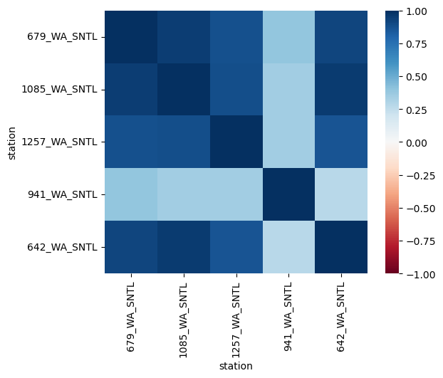
../../_images/f6438f1062281e39d8b7695e11554882a6eccc8be172eed6ea7bf383839e9861.png

Now we’ll use `.corr()` to calculate the correlation values for different combinations of stations, and seaborn’s heatmap function to plot the correlation matrix#

#The Pandas `corr` should properly handle nans
snwd_corr = all_stations_snwd_df[site_list].corr()
snwd_corr

station	679_WA_SNTL	1085_WA_SNTL	1257_WA_SNTL	941_WA_SNTL	642_WA_SNTL
station
679_WA_SNTL	1.000000	0.946617	0.878109	0.397001	0.916370
1085_WA_SNTL	0.946617	1.000000	0.890231	0.350175	0.958519
1257_WA_SNTL	0.878109	0.890231	1.000000	0.350870	0.861648
941_WA_SNTL	0.397001	0.350175	0.350870	1.000000	0.281228
642_WA_SNTL	0.916370	0.958519	0.861648	0.281228	1.000000

sns.heatmap(snwd_corr, cmap='RdBu', vmin=-1, vmax=1, square=True);

../../_images/345712ea004d3eaaa1d94c1a1230dee44c4b63b6f7cd550d4911a0363b092c3e.png

How does the correlation coefficient change with distance?#

Select the Paradise station as your reference station

ref_site = '679_WA_SNTL'
equidist_crs = 'ESRI:102005'

Compute the following…#

corr_with_ref_site_df
- Correlation score with your reference station
dist_from_ref_site_km_df
- Distance in km from your reference station
- Hint: Try geopandas .distance function we used in lab05
- Use the equidistant crs provided above for the distance calculation
elev_diff_from_ref_site_m_df
- Elevation difference of the sites minus the reference site

# STUDENT CODE HERE

all_stations_gdf['corr_with_ref_site'] = corr_with_ref_site_df
all_stations_gdf['dist_from_ref_site_km'] = dist_from_ref_site_km_df
all_stations_gdf['elev_diff_from_ref_site_m'] = elev_diff_from_ref_site_m_df

Create a map with values representing correlation with the reference site#

# STUDENT CODE HERE

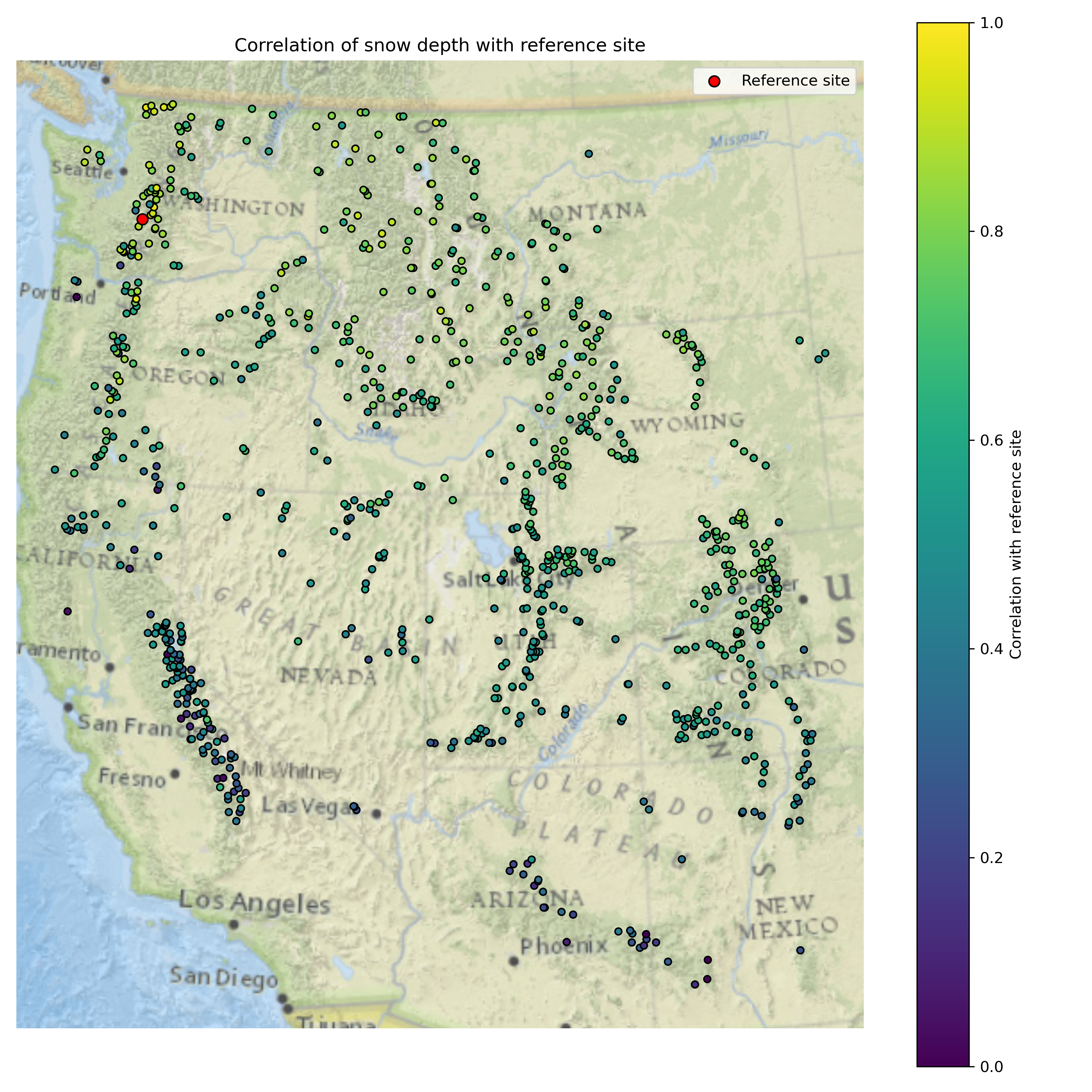
../../_images/snotel_snwd_corr_with_ref_site.png

Written response: How does the correlation score vary with distance from the reference site? How does this relate to Tobler’s first law and the idea of spatial autocorrelation?#

STUDENT WRITTEN RESPONSE HERE

Create a plot of correlation scores with the reference site, with distance from site on the x-axis, and elevation difference from reference site on the y-axis#

# STUDENT CODE HERE

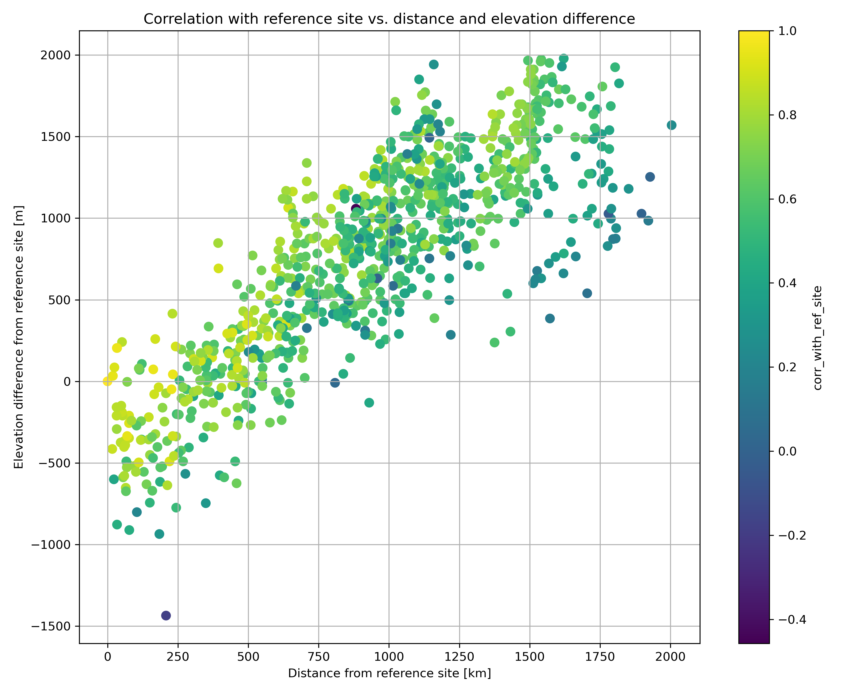
../../_images/snotel_snwd_corr_vs_dist_elev.png

Written response: If our reference station at Paradise broke, yet you needed to know the snow depth there, what factors would you consider when choosing a different site to use as a proxy?#

STUDENT WRITTEN RESPONSE HERE

Part 4: Western U.S. long-term snow depth statistics (3 pts)#

Now that we’ve analyzed temporal variability, let’s look at long-term aggregations. We previously filtered out snow depths less than 1 centimeter and greater than 10 meters which improve some of these calculations.

At each site, calculate…#

the long-term median snow depth
the long-term max snow depth
the 2024 water year max snow depth
recent snow depth (2025-02-23)
percent normal snow depth (2025-02-23)

# STUDENT CODE HERE

# STUDENT CODE HERE

Plot the variables you just calculated!#

# STUDENT CODE HERE

../../_images/snotel_long_term_median.png

../../_images/snotel_wateryear2024_max.png

../../_images/snotel_recent_depth_pct_norm.png

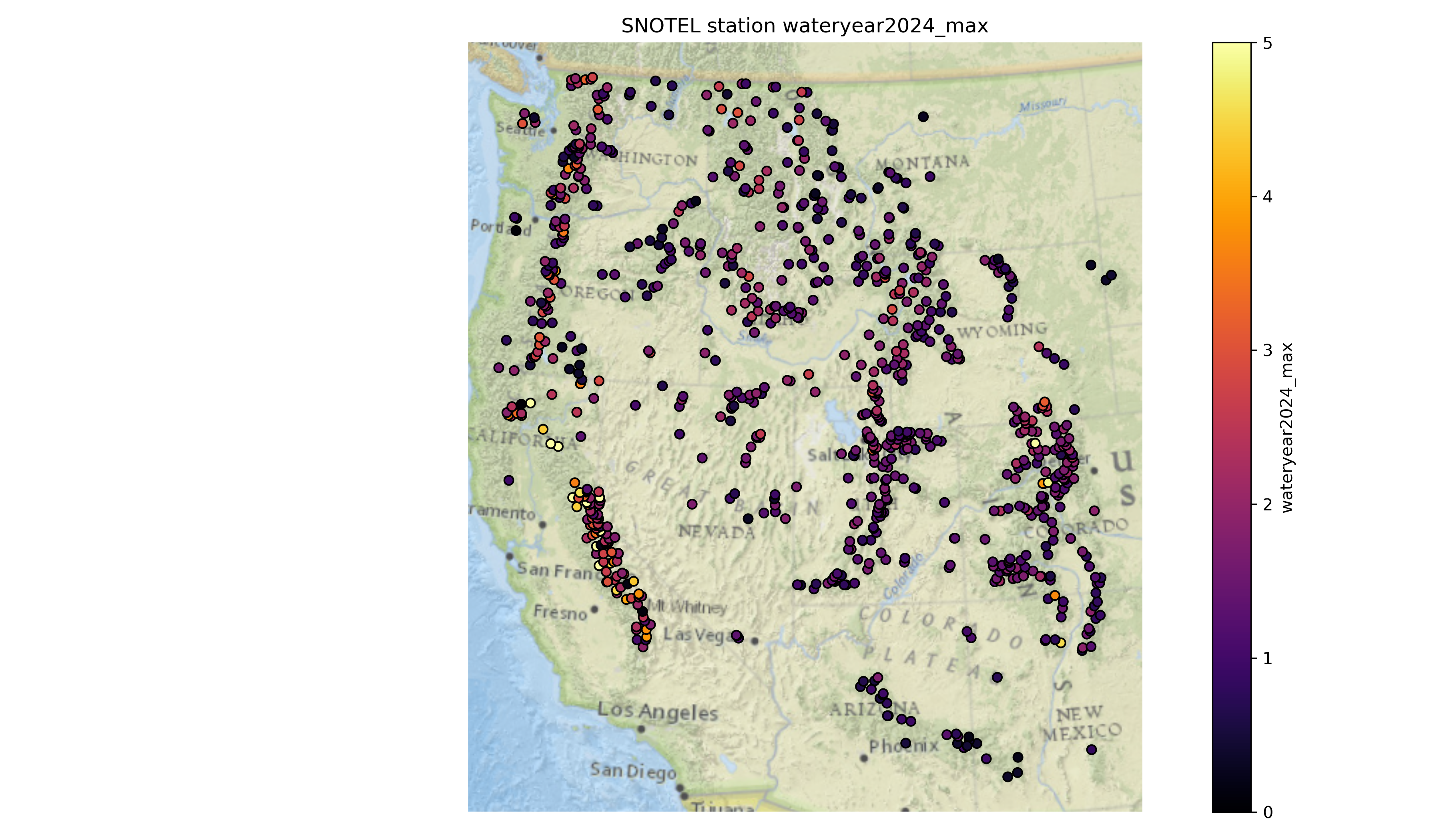
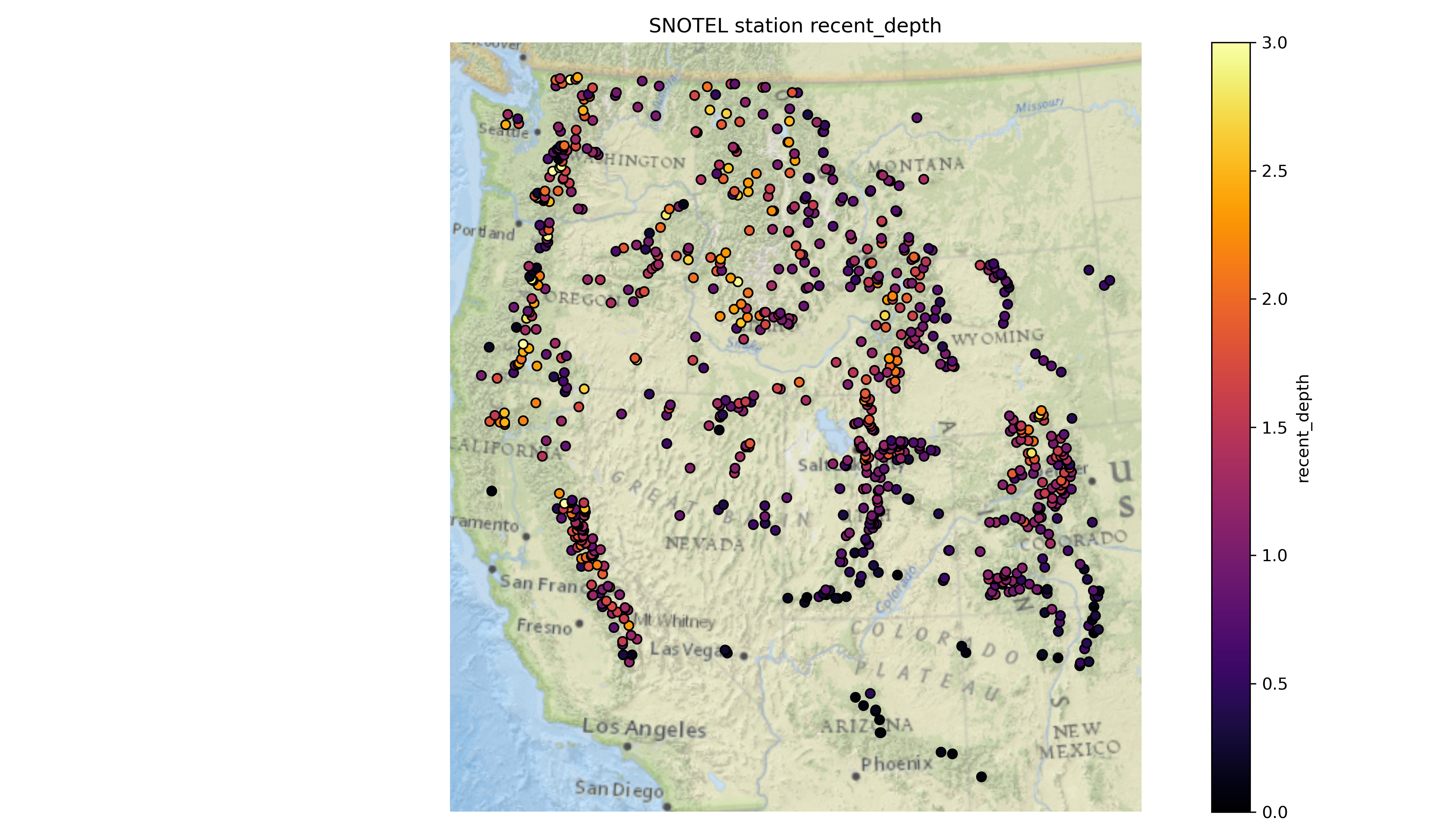
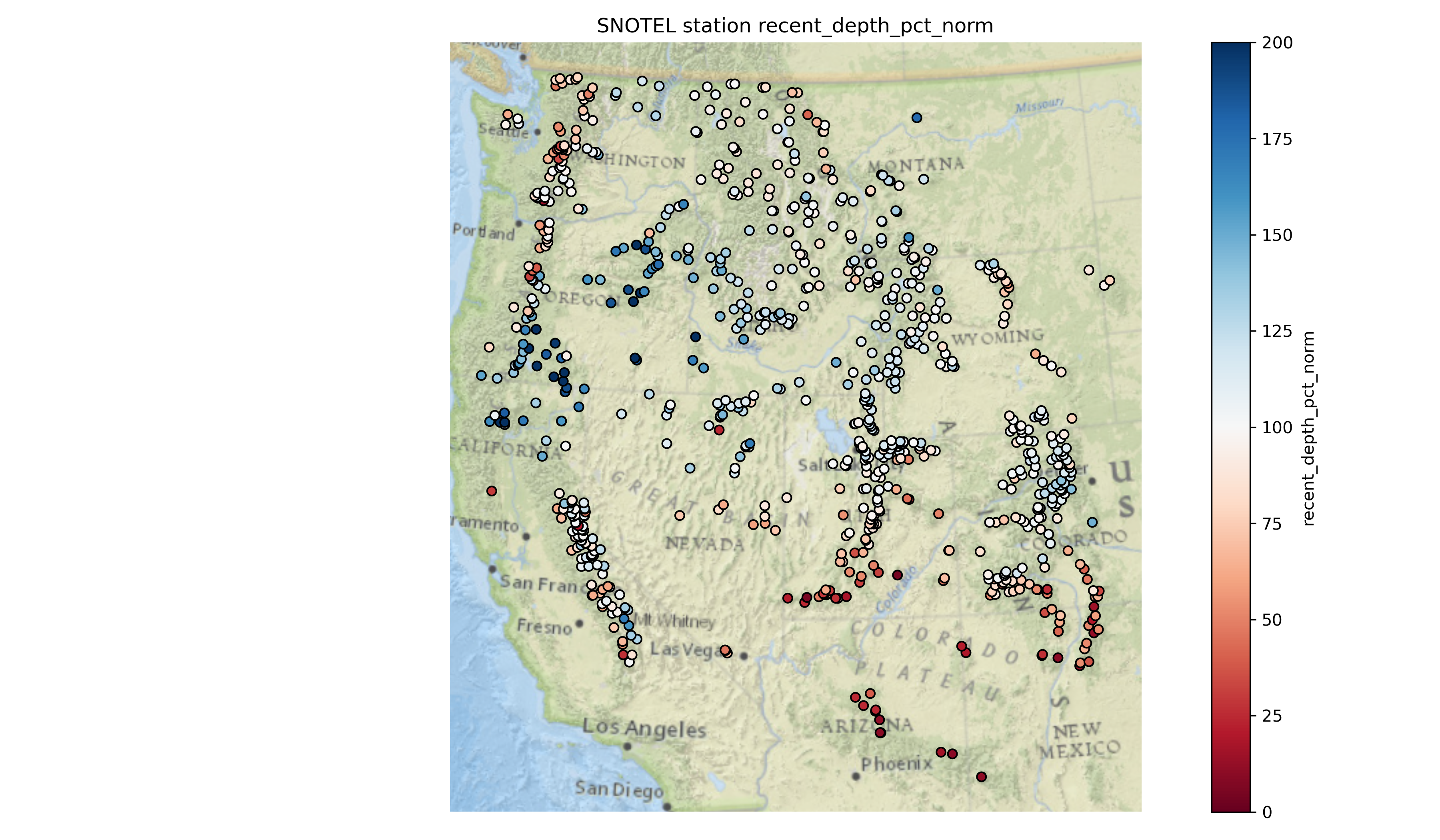
Written response: According to the percent of normal snow depth plot, what areas currently have a lower snow depth value than usual for this time of year? What areas have higher values than usual?#

STUDENT WRITTEN RESPONSE HERE

Part 5: Spatial autocorrelation and interpolation (4 pts)#

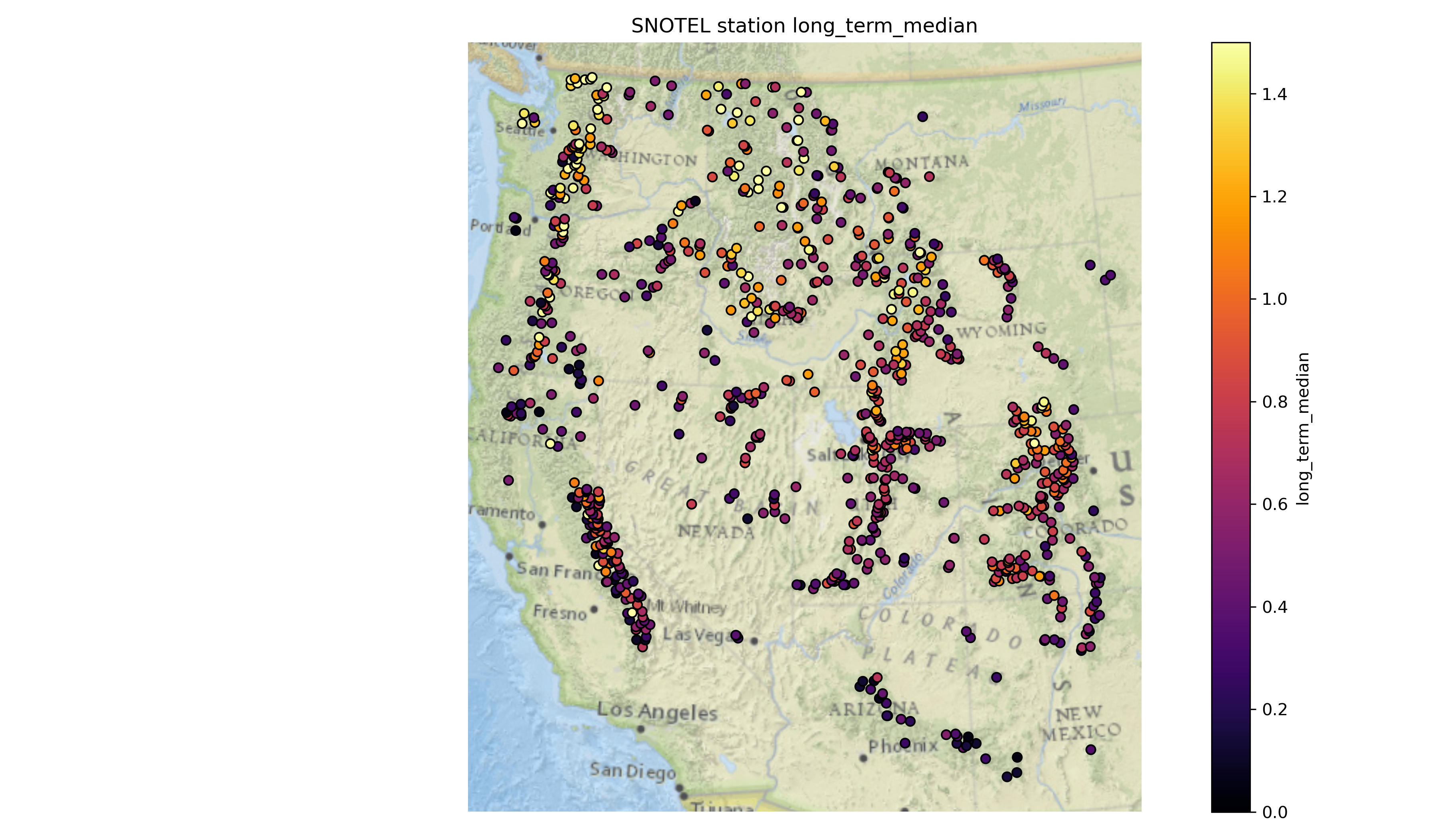
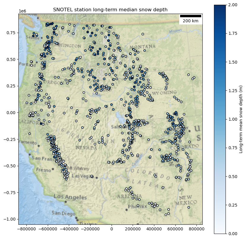
For this part, you’ll want to refer back to the module 08 demo. Let’s take a look at the long-term median snow depth…

# Let's quickly remove stations with no long term median value
stations_filtered_gdf = all_stations_gdf[['long_term_median','geometry']].dropna()

f,ax=plt.subplots(figsize=(10,10))
stations_filtered_gdf.plot(ax=ax,
                      column='long_term_median', 
                      cmap='Blues', 
                      legend=True, 
                      legend_kwds={'label': 'Long-term mean snow depth (m)'}, 
                      edgecolor='k',
                      markersize=25,
                      vmin=0,
                      vmax=2)
ax.add_artist(ScaleBar(1, location='upper right', units='m'))
ctx.add_basemap(ax, crs=stations_filtered_gdf.crs, source=ctx.providers.Esri.NatGeoWorldMap, alpha=0.7, attribution=False)
ax.set_title('SNOTEL station long-term median snow depth')

Text(0.5, 1.0, 'SNOTEL station long-term median snow depth')

../../_images/76aa121eb0d6ca697ca5070c936ef03a140f05a251af4d5b05800e337300b687.png

Check for autocorrelation using Global Moran’s I#

Try two different ways of specifying your weights / connectivity!

y = stations_filtered_gdf['long_term_median'].values

k = 8  # Number of neighbors
w = weights.KNN.from_dataframe(stations_filtered_gdf, k=k)

# or define w based on distance
dist_threshold = 100*1000
w = weights.distance.DistanceBand.from_dataframe(stations_filtered_gdf, threshold=dist_threshold)

w.transform = 'r'  

('WARNING: ', '933_NM_SNTL', ' is an island (no neighbors)')
('WARNING: ', '1034_NM_SNTL', ' is an island (no neighbors)')
('WARNING: ', '917_MT_SNTL', ' is an island (no neighbors)')
('WARNING: ', 'NLS', ' is an island (no neighbors)')

/home/eric/miniconda3/envs/uwgda2025/lib/python3.12/site-packages/libpysal/weights/util.py:826: UserWarning: The weights matrix is not fully connected: 
 There are 13 disconnected components.
 There are 4 islands with ids: 933_NM_SNTL, 1034_NM_SNTL, 917_MT_SNTL, NLS.
  w = W(neighbors, weights, ids, **kwargs)
/home/eric/miniconda3/envs/uwgda2025/lib/python3.12/site-packages/libpysal/weights/distance.py:844: UserWarning: The weights matrix is not fully connected: 
 There are 13 disconnected components.
 There are 4 islands with ids: 933_NM_SNTL, 1034_NM_SNTL, 917_MT_SNTL, NLS.
  W.__init__(

# STUDENT CODE HERE

Written response: What did you calculate for your Global Moran’s I, and how do you interpret your results?#

STUDENT WRITTEN RESPONSE HERE

Now calculate Local Moran’s I#

# STUDENT CODE HERE

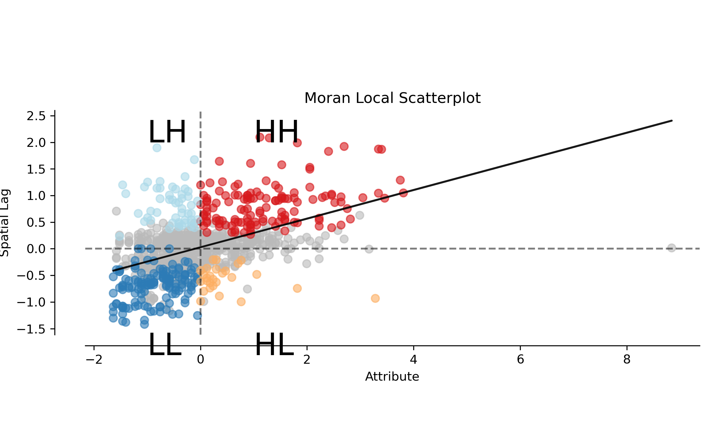
Make a scatterplot for Moran’s I#

# STUDENT CODE HERE

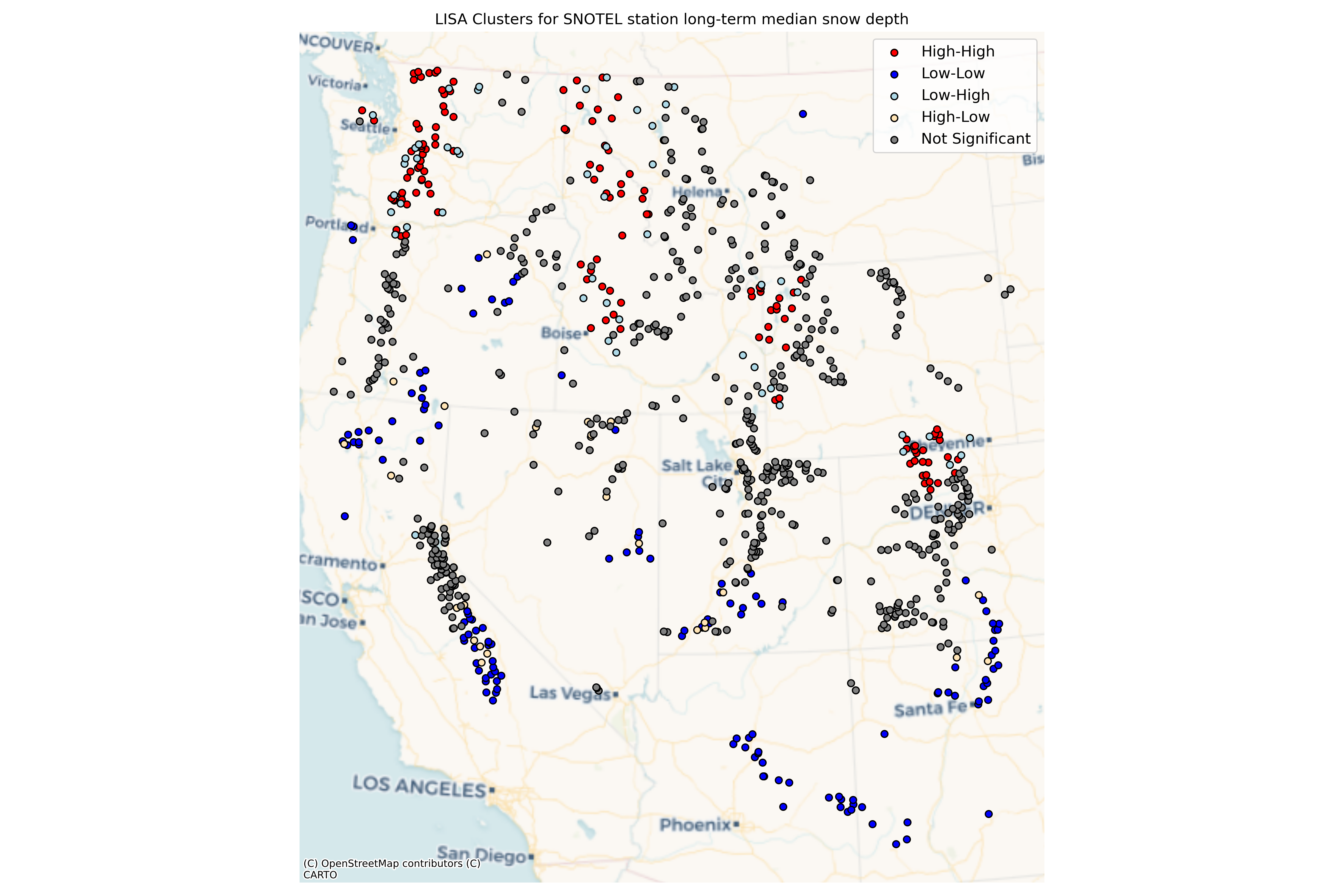
Plot your Local Moran’s I clusters on a map#

# STUDENT CODE HERE

# STUDENT CODE HERE

# Calculate percentage of each cluster type
total_sig = sum(stations_filtered_lisa['significant'])
for cluster_type in ['High-High', 'Low-Low', 'Low-High', 'High-Low']:
    count = sum(stations_filtered_lisa['cluster_type'] == cluster_type)
    percent = count / total_sig * 100 if total_sig > 0 else 0
    print(f"{cluster_type}: {count} points ({percent:.1f}% of significant clusters)")

# Interpret results
print("\nInterpretation of LISA clusters:")
print("- High-High clusters (hotspots): Areas with high snow depth surrounded by areas with high snow depth")
print("- Low-Low clusters (coldspots): Areas with low snow depth surrounded by areas with low snow depth")
print("- Low-High clusters: Areas with low snow depth surrounded by areas with high snow depth")
print("- High-Low clusters: Areas with high snow depth surrounded by areas with low snow depth")

High-High: 132 points (37.9% of significant clusters)
Low-Low: 139 points (39.9% of significant clusters)
Low-High: 50 points (14.4% of significant clusters)
High-Low: 27 points (7.8% of significant clusters)

Interpretation of LISA clusters:
- High-High clusters (hotspots): Areas with high snow depth surrounded by areas with high snow depth
- Low-Low clusters (coldspots): Areas with low snow depth surrounded by areas with low snow depth
- Low-High clusters: Areas with low snow depth surrounded by areas with high snow depth
- High-Low clusters: Areas with high snow depth surrounded by areas with low snow depth

Written response: How do you interpret your Local Moran’s I, and how does your choice of connectivity affect your results?#

STUDENT WRITTEN RESPONSE HERE

Now create and plot a variogram using the demo as a guide. Use n_lags of 50. Experiment with maxlags of 1km, 10km, 100km, 1,000km, 10,000km to see how the variogram and its range changes. For the purposes of this question’s output and the rest of the lab, proceed with a maxlag of 100km.#

# STUDENT CODE HERE

Calculating empirical variogram...
Fitting variogram model...

# STUDENT CODE HERE

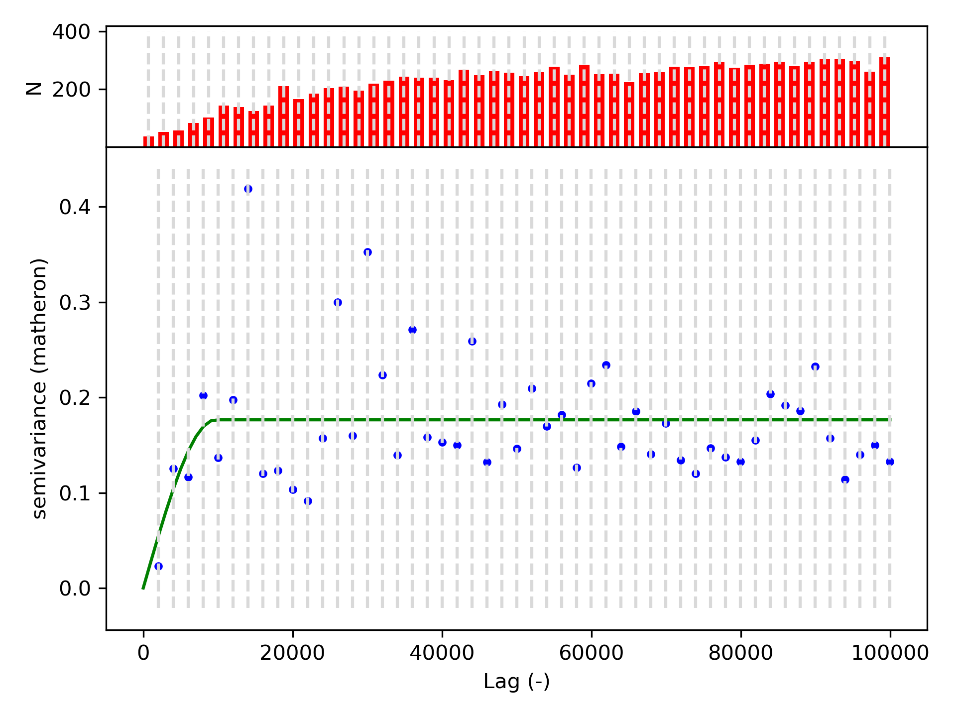
Print out the variogram model parameters#

# STUDENT CODE HERE

Variogram Model Parameters:
Model type: spherical
Nugget: 0.0000
Sill: 0.1765
Effective range: 9.6665 km

How did varying the maxlag affect your variogram and effective range? What does this sensitivity to maximum lag distance suggest? For the variogram you proceeded with (maxlag of 100km), interpret the effective range. What is this saying about snow depth physically, and does this match your intuition?#

Hint: When thinking about the sensitivity to maximum lag distance, revisit the reading on variogram calculation, specifically paying attention to stationarity and the brick example

STUDENT WRITTEN RESPONSE HERE

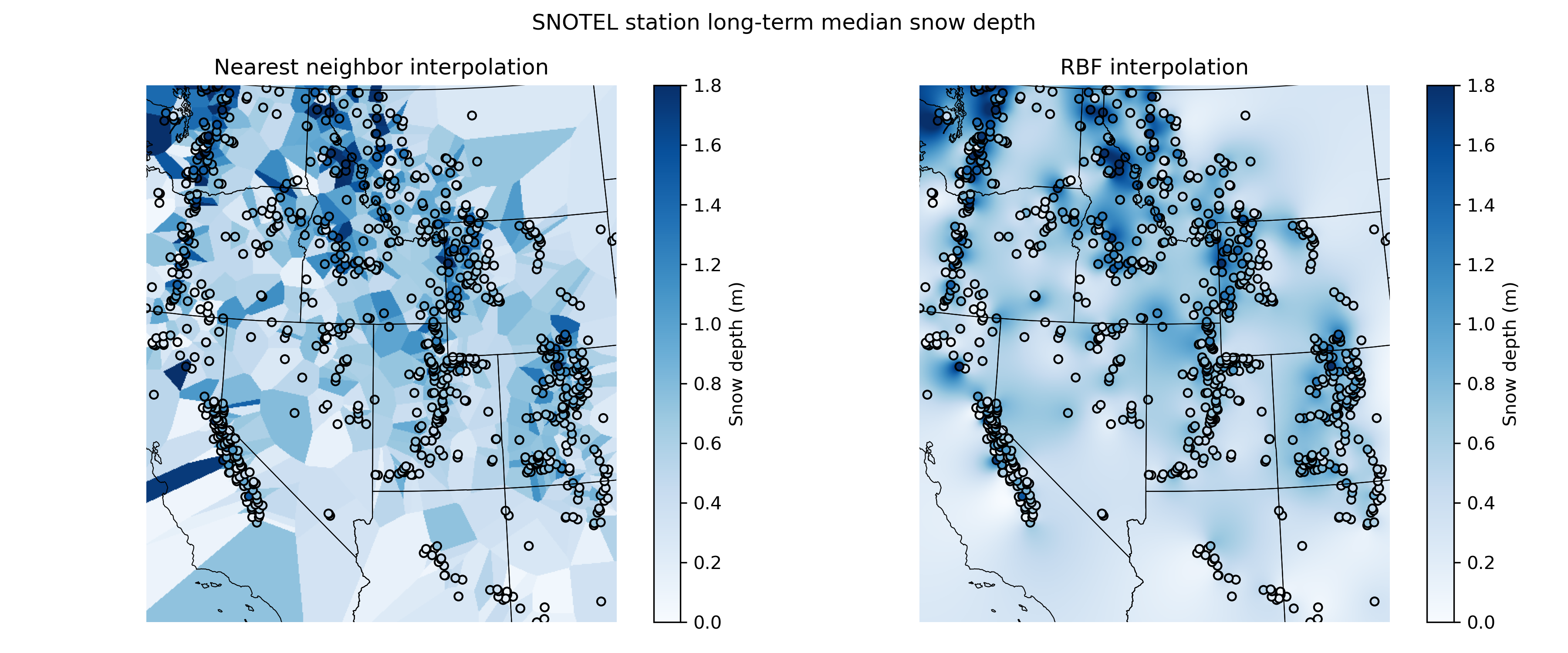
Now try interpolating the sparse snow depth points and plot a median snow depth raster using two deterministic interpolation methods, nearest interpolation and radial basis functions with a linear kernel#

For context, plot the states underneath and also the median snow depth point values (use the same colorbar as the raster)

x = coords[:,0]
y = coords[:,1]
z = values

bounds = stations_filtered_gdf.total_bounds
dx,dy = (3000,3000)

mpl_extent = (bounds[0],bounds[2],bounds[1],bounds[3])


xi = np.arange(np.floor(bounds[0]), np.ceil(bounds[2]),dx)
yi = np.arange(np.ceil(bounds[3]),np.floor(bounds[1]),-dy)
xx, yy = np.meshgrid(xi, yi)

interp_func_rbf = scipy.interpolate.Rbf(x, y, z, function='linear')
interp_rbf = interp_func_rbf(xx, yy)
interp_nearest = scipy.interpolate.griddata((x,y), z, (xx, yy), method='nearest')

# STUDENT CODE HERE

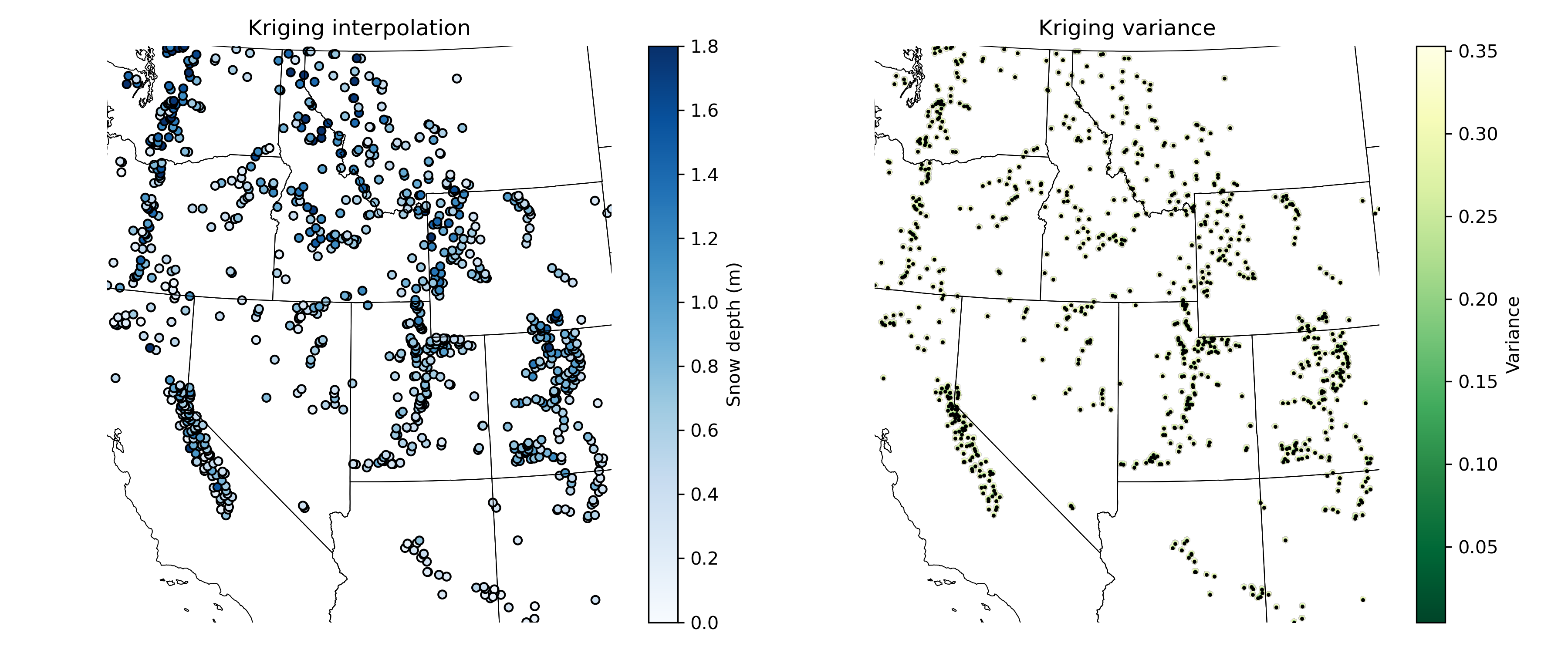
../../_images/snotel_snwd_interpolation.png

Finally, use the variogram you created to do Kriging interpolation and plot a median snow depth raster#

ok = skg.OrdinaryKriging(V, min_points=1, max_points=15, mode='exact')
field = ok.transform(xx.flatten(), yy.flatten()).reshape(xx.shape)
s2 = ok.sigma.reshape(xx.shape)

Warning: for 292311 locations, not enough neighbors were found within the range.

# STUDENT CODE HERE

f,axs=plt.subplots(1,3,figsize=(15,5))

axs[0].imshow(interp_nearest, extent=mpl_extent, cmap='Blues',vmin=0,vmax=1.8)
axs[0].set_title('Nearest neighbor interpolation')

axs[1].imshow(interp_rbf, extent=mpl_extent, cmap='Blues',vmin=0,vmax=1.8)
axs[1].set_title('RBF interpolation')

axs[2].imshow(field, extent=mpl_extent, cmap='Blues', vmin=0, vmax=1.8)
axs[2].set_title('Kriging interpolation')

for ax in axs:
    ax.set_xlim(bounds[0],bounds[2])
    ax.set_ylim(bounds[1],bounds[3])
    states_gdf.boundary.plot(ax=ax, color='k', linewidth=0.5)
    stations_filtered_gdf.plot(ax=ax, column='long_term_median', cmap='Blues', legend=True, legend_kwds={'label': 'Snow depth (m)'}, markersize=0.1, vmin=0, vmax=1.8, edgecolor='k')
    ax.set_aspect('equal')
    ax.axis('off')

f.tight_layout()

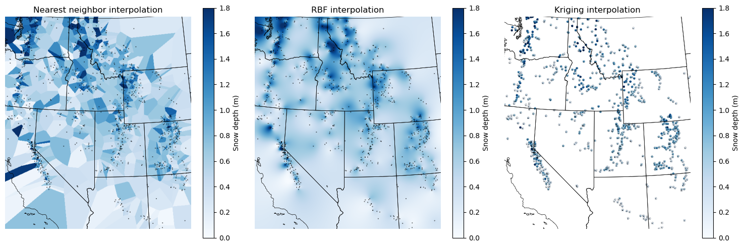
../../_images/d7523fd3c2ed93898d7e5dc60bb8554e4e79545e981357e4d5432ecc2cca40d1.png

Written response: Interpret your interpolations! For each interpolation, describe a use case where you’d prefer this interpolation over the other two. For the Kriging interpolation, why are only small areas around the points interpolated?#

STUDENT WRITTEN RESPONSE HERE

Submission#

Save the completed notebook (make sure to fully run the notebook and check all cell output is visible)
Use the git add; git commit -m 'message'; git push workflow to push your work to the remote repository
- ideally you’ve been using add / commit / push as you make progress on this notebook
Check the remote repository to check all of the files you want to submit have been pushed
Scroll through your jupyter notebook on your remote repository and make sure all output and plots are visible
When you have completed your last push, submit the url pointing to your Github repository to the corresponding Canvas assignment

Lab 08 assignment (20 pts)

Contents

Lab 08 assignment (20 pts)#

Introduction#

Objectives#

Instructions#

Part 0: Imports and filenames#

First, let’s import the libraries we’ll need. Make sure to shut down any other kernels you have running!#

Part 1: Explore the SNOTEL sites (4 pts)#

Load SNOTEL sites geojson#

Let’s quickly visualize with .explore()#

Written response: Where are station locations the most dense? Are there any areas you think are undersampled?#

Load in state data, filter out Alaska stations, and reproject#

Remove stations in Alaska from the all_stations_gdf#

Calculate the convex hull of the remaining stations. Create an Albers Equal Area projection string, using the center of the convex hull as the center lat and lon, and the min and max latitude bound of the convex hull as the standard parallels.#

Reproject our stations and states geodataframes to this new projection, and then create a plot of SNOTEL station locations and elevations overlaid on the states geometries and a basemap.#

Print the station name, code, latitude, longitude, state, and elevation of the highest and lowest stations#

Create wa_stations_gdf, a geodataframe of just the stations in Washington. Create a figure with three plots: a map of all of the stations (still excluding Alaska), a map of the Washington stations, and then one plot with their respective elevation histograms.#

Written response: Imagine using traditional statistical tests to answer each of the following questions. For each, comment on whether you think spatial autocorrelation is a concern and why. For traditional statistics, what assumptions are violated due to spatial autocorrelation?#

Part 2: Single site time series analysis and temporal autocorrelation (5 pts)#

Index into snotel_ds to load data from Paradise site (ID 679) on Mt. Rainer as paradise_snotel_ds#

Here we’ll use the .to_pandas() function to turn our xarray dataset into a pandas dataframe#

Written response: You’ll notice we preserved the WY and DOWY columns. Read the water year wikipedia page. Why might water year and day of water year (DOWY) be useful for us when comparing snow hydrology data?#

Plot snow depth vs day of water year, with colors representing average temperatures#

Compute statistics for each day of water year, using values from all years#

What day of water year has the highest average snow depth, and what is that snow depth? What calendar day does this correspond to?#

Create a plot of these aggregated dowy values, and add the current water year’s daily data as a scatter plot on top#

For most recent snow depth value in the record, what is the percentage of “normal”#

Now let’s view the data as time-series plots#

Create a figure to plot snow depth, temperature, and precipitation for water year 2021#

Now we’ll calculate the temporal autocorrelation for WY 2021…#

Now plot the same variables, but this time use the full time-series#

Now we’ll calculate the temporal autocorrelation for the entire time-series…#

What would the variogram for snow depth look like here??#

Part 3: Western U.S. time-series analysis and correlation (4 pts)#

Inspect the SNOTEL dataset#

Create all_stations_snwd_df, a pandas dataframe of snow depth at all stations, with each row representing a day, and each column representing a station#

Create a plot of total operational stations vs time#

Create a histogram of all snow depth values#

Hmmm, let’s filter out snow depth values less than one centimeter and greater than 10 meters. This will help with our aggregations later, as well as remove unlikely values.#

Use the built-in .describe() function to determine look at some quick statistics. Which station has the highest mean snow depth? Which station has the greatest number of days with snow depth data?#

Temporal correlation of snow depth for nearby stations#

Now we’ll use .corr() to calculate the correlation values for different combinations of stations, and seaborn’s heatmap function to plot the correlation matrix#

How does the correlation coefficient change with distance?#

Compute the following…#

Create a map with values representing correlation with the reference site#

Written response: How does the correlation score vary with distance from the reference site? How does this relate to Tobler’s first law and the idea of spatial autocorrelation?#

Create a plot of correlation scores with the reference site, with distance from site on the x-axis, and elevation difference from reference site on the y-axis#

Written response: If our reference station at Paradise broke, yet you needed to know the snow depth there, what factors would you consider when choosing a different site to use as a proxy?#

Part 4: Western U.S. long-term snow depth statistics (3 pts)#

At each site, calculate…#

Plot the variables you just calculated!#

Written response: According to the percent of normal snow depth plot, what areas currently have a lower snow depth value than usual for this time of year? What areas have higher values than usual?#

Part 5: Spatial autocorrelation and interpolation (4 pts)#

Check for autocorrelation using Global Moran’s I#

Written response: What did you calculate for your Global Moran’s I, and how do you interpret your results?#

Now calculate Local Moran’s I#

Make a scatterplot for Moran’s I#

Plot your Local Moran’s I clusters on a map#

Written response: How do you interpret your Local Moran’s I, and how does your choice of connectivity affect your results?#

Now create and plot a variogram using the demo as a guide. Use n_lags of 50. Experiment with maxlags of 1km, 10km, 100km, 1,000km, 10,000km to see how the variogram and its range changes. For the purposes of this question’s output and the rest of the lab, proceed with a maxlag of 100km.#

Print out the variogram model parameters#

Now try interpolating the sparse snow depth points and plot a median snow depth raster using two deterministic interpolation methods, nearest interpolation and radial basis functions with a linear kernel#

Finally, use the variogram you created to do Kriging interpolation and plot a median snow depth raster#

Written response: Interpret your interpolations! For each interpolation, describe a use case where you’d prefer this interpolation over the other two. For the Kriging interpolation, why are only small areas around the points interpolated?#

Submission#

Let’s quickly visualize with `.explore()`#

Remove stations in Alaska from the `all_stations_gdf`#

Create `wa_stations_gdf`, a geodataframe of just the stations in Washington. Create a figure with three plots: a map of all of the stations (still excluding Alaska), a map of the Washington stations, and then one plot with their respective elevation histograms.#

Index into `snotel_ds` to load data from Paradise site (ID 679) on Mt. Rainer as `paradise_snotel_ds`#

Here we’ll use the `.to_pandas()` function to turn our xarray dataset into a pandas dataframe#

Written response: You’ll notice we preserved the `WY` and `DOWY` columns. Read the water year wikipedia page. Why might water year and day of water year (DOWY) be useful for us when comparing snow hydrology data?#

Create `all_stations_snwd_df`, a pandas dataframe of snow depth at all stations, with each row representing a day, and each column representing a station#

Use the built-in `.describe()` function to determine look at some quick statistics. Which station has the highest mean snow depth? Which station has the greatest number of days with snow depth data?#

Now we’ll use `.corr()` to calculate the correlation values for different combinations of stations, and seaborn’s heatmap function to plot the correlation matrix#