Lab 04 assignment notebook 1 (20 pts)#
Notebook 1 of 2
UW Geospatial Data Analysis
CEE467/CEWA567
David Shean, Eric Gagliano, Quinn Brencher
Introduction#
This lab focuses on solidifying your understanding of fundamental raster concepts. You will…
inspect, read, and write raster data
understand raster attributes
perform quantitative analysis such as band math operations and thresholding
practice different raster visualization approaches
Instructions#
Please go through all cells in the notebook sequentially, making sure to complete all instructions
Some answers are left in as a guide–you still need to fill in the code to produce the output on your own!
Answers should be produced using code unless otherwise noted by “Written response”
Follow submission instructions closely, making sure you save and submit your notebook with all your outputs preserved
Part 0: Imports and filenames#
First, let’s import the libraries we’ll need.#
import geopandas as gpd
import rasterio as rio
import rioxarray as rxr
import matplotlib.pyplot as plt
from matplotlib_scalebar.scalebar import ScaleBar
from pathlib import Path
import os
import pyproj
import numpy as np
#May want to use interactive plotting for zoom/pan and live coordinate display
#%matplotlib widget
%matplotlib inline
Let’s make sure our files are where we think they are!#
If you haven’t downloaded the files already, please run the download demo notebook.
imgdir = f'{Path.home()}/gda_demo_data/LS8_data'
!ls -lh $imgdir
total 1.3G
-rw-r--r-- 1 eric eric 1.2M Jan 26 11:31 LC08_L2SP_046027_20180818_02_T1_rendered_preview.png
-rw-r--r-- 1 eric eric  81M Jan 26 11:27 LC08_L2SP_046027_20180818_20200831_02_T1_SR_B1.TIF
-rw-r--r-- 1 eric eric  81M Jan 26 11:28 LC08_L2SP_046027_20180818_20200831_02_T1_SR_B2.TIF
-rw-r--r-- 1 eric eric  82M Jan 26 11:28 LC08_L2SP_046027_20180818_20200831_02_T1_SR_B3.TIF
-rw-r--r-- 1 eric eric  83M Jan 26 11:29 LC08_L2SP_046027_20180818_20200831_02_T1_SR_B4.TIF
-rw-r--r-- 1 eric eric  92M Jan 26 11:29 LC08_L2SP_046027_20180818_20200831_02_T1_SR_B5.TIF
-rw-r--r-- 1 eric eric  90M Jan 26 11:30 LC08_L2SP_046027_20180818_20200831_02_T1_SR_B6.TIF
-rw-r--r-- 1 eric eric  84M Jan 26 11:31 LC08_L2SP_046027_20180818_20200831_02_T1_ST_B10.TIF
-rw-r--r-- 1 eric eric 115M Jan 27 19:39 LC08_L2SP_046027_20180818_20200831_02_T1_ST_B10_4326.TIF
-rw-r--r-- 1 eric eric 1.5M Jan 26 11:27 LC08_L2SP_046027_20181224_02_T1_rendered_preview.png
-rw-r--r-- 1 eric eric  91M Jan 26 11:23 LC08_L2SP_046027_20181224_20200829_02_T1_SR_B1.TIF
-rw-r--r-- 1 eric eric  91M Jan 26 11:24 LC08_L2SP_046027_20181224_20200829_02_T1_SR_B2.TIF
-rw-r--r-- 1 eric eric  92M Jan 26 11:24 LC08_L2SP_046027_20181224_20200829_02_T1_SR_B3.TIF
-rw-r--r-- 1 eric eric  91M Jan 26 11:25 LC08_L2SP_046027_20181224_20200829_02_T1_SR_B4.TIF
-rw-r--r-- 1 eric eric  96M Jan 26 11:26 LC08_L2SP_046027_20181224_20200829_02_T1_SR_B5.TIF
-rw-r--r-- 1 eric eric  90M Jan 26 11:26 LC08_L2SP_046027_20181224_20200829_02_T1_SR_B6.TIF
-rw-r--r-- 1 eric eric  77M Jan 26 11:27 LC08_L2SP_046027_20181224_20200829_02_T1_ST_B10.TIF
Let’s assign band filenames to variables#
#Pre-identified cloud-free Image IDs used for the lab
august_id = 'LC08_L2SP_046027_20180818_20200831_02_T1' # August 2018
december_id = 'LC08_L2SP_046027_20181224_20200829_02_T1' # # December 2018
We’ve done the thermal infrared, shortwave infrared, and near infrared for you.
# B10 is the thermal infrared /surface temperture band
tir_august_fn = os.path.join(imgdir, august_id+'_ST_B10.TIF')
tir_december_fn = os.path.join(imgdir, december_id+'_ST_B10.TIF')

swir_august_fn = os.path.join(imgdir, august_id+'_SR_B6.TIF')
swir_december_fn = os.path.join(imgdir, december_id+'_SR_B6.TIF')

nir_august_fn = os.path.join(imgdir, august_id+'_SR_B5.TIF')
nir_december_fn = os.path.join(imgdir, december_id+'_SR_B5.TIF')
Please add variables for red, green, and blue each of the two images.#
If you’re unsure of which filename corresponds to each band, check the chart in the download demo notebook.
# STUDENT CODE HERE
Written response: Use gdalinfo to inspect the blue band from the december image, and report which CRS this image is in.#
# STUDENT CODE HERE
STUDENT WRITTEN RESPONSE HERE
Part 1: Raster basics (2 pts)#
Before we switch to rioxarray for the remainder of the lab, let’s briefly open and read in the near infrared band from the August 2018 image with rasterio.#
nir_august_src = rio.open(nir_august_fn)
nir_august_src.profile
{'driver': 'GTiff', 'dtype': 'uint16', 'nodata': 0.0, 'width': 7771, 'height': 7891, 'count': 1, 'crs': CRS.from_wkt('PROJCS["WGS 84 / UTM zone 10N",GEOGCS["WGS 84",DATUM["WGS_1984",SPHEROID["WGS 84",6378137,298.257223563,AUTHORITY["EPSG","7030"]],AUTHORITY["EPSG","6326"]],PRIMEM["Greenwich",0,AUTHORITY["EPSG","8901"]],UNIT["degree",0.0174532925199433,AUTHORITY["EPSG","9122"]],AUTHORITY["EPSG","4326"]],PROJECTION["Transverse_Mercator"],PARAMETER["latitude_of_origin",0],PARAMETER["central_meridian",-123],PARAMETER["scale_factor",0.9996],PARAMETER["false_easting",500000],PARAMETER["false_northing",0],UNIT["metre",1,AUTHORITY["EPSG","9001"]],AXIS["Easting",EAST],AXIS["Northing",NORTH],AUTHORITY["EPSG","32610"]]'), 'transform': Affine(30.0, 0.0, 473685.0,
       0.0, -30.0, 5373615.0), 'blockxsize': 256, 'blockysize': 256, 'tiled': True, 'compress': 'deflate', 'interleave': 'band'}
Written response: Based on this inspection of the metadata, how do you think missing values are represented?#
STUDENT WRITTEN RESPONSE HERE
Unmasked…#
nir_august_ar = nir_august_src.read(1)
nir_august_ar
array([[0, 0, 0, ..., 0, 0, 0],
       [0, 0, 0, ..., 0, 0, 0],
       [0, 0, 0, ..., 0, 0, 0],
       ...,
       [0, 0, 0, ..., 0, 0, 0],
       [0, 0, 0, ..., 0, 0, 0],
       [0, 0, 0, ..., 0, 0, 0]], dtype=uint16)
Masked…#
nir_august_ma = nir_august_src.read(1,masked=True)
nir_august_ma
masked_array(
  data=[[--, --, --, ..., --, --, --],
        [--, --, --, ..., --, --, --],
        [--, --, --, ..., --, --, --],
        ...,
        [--, --, --, ..., --, --, --],
        [--, --, --, ..., --, --, --],
        [--, --, --, ..., --, --, --]],
  mask=[[ True,  True,  True, ...,  True,  True,  True],
        [ True,  True,  True, ...,  True,  True,  True],
        [ True,  True,  True, ...,  True,  True,  True],
        ...,
        [ True,  True,  True, ...,  True,  True,  True],
        [ True,  True,  True, ...,  True,  True,  True],
        [ True,  True,  True, ...,  True,  True,  True]],
  fill_value=0,
  dtype=uint16)
print(f'Unmasked array dtype: {nir_august_ar.dtype}, nodata value: {int(nir_august_src.profile["nodata"])}, size: {nir_august_ar.nbytes/1e6:.2f} MB')
print('-----------------------------------------------------------------------------------')
print(f'Masked array (just the data array) dtype: {nir_august_ma.dtype}, nodata value: {nir_august_ma.fill_value}, size: {nir_august_ma.nbytes/1e6:.2f} MB')
print(f'Accompanying mask dtype: {nir_august_ma.mask.dtype}, size: {nir_august_ma.mask.nbytes/1e6:.2f} MB')
print(f'Combined masked array (data array+mask) size: {(nir_august_ma.nbytes/1e6 + nir_august_ma.mask.nbytes/1e6):.2f} MB')
Unmasked array dtype: uint16, nodata value: 0, size: 122.64 MB
-----------------------------------------------------------------------------------
Masked array (just the data array) dtype: uint16, nodata value: 0, size: 122.64 MB
Accompanying mask dtype: bool, size: 61.32 MB
Combined masked array (data array+mask) size: 183.96 MB
Written response: Compare the amount of memory the unmasked array takes up in memory vs how much memory the respective file takes up on the disk (see !ls -lh $imgdir output above). Why might these be different?#
STUDENT WRITTEN RESPONSE HERE
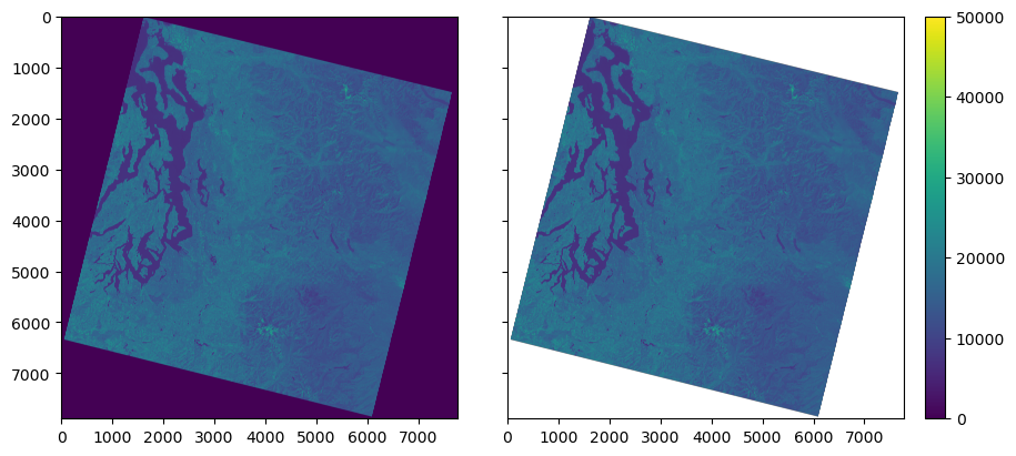
f,axs=plt.subplots(1,2, figsize=(9,4),sharey=True, layout='constrained')

axs[0].imshow(nir_august_ar,vmin=0,vmax=50000)
im = axs[1].imshow(nir_august_ma,vmin=0,vmax=50000)

f.colorbar(im)
<matplotlib.colorbar.Colorbar at 0x7efce0001af0>
nir_august_src.close()
nir_august_ar = None
nir_august_ma = None
Written response: What differences did you notice between the unmasked and masked ouputs and plots? Do the dark purple regions in the unmasked array reflect real values?#
STUDENT WRITTEN RESPONSE HERE
Now we’ll do the same thing, but using rioxarray…#
nir_august_unmasked_da = rxr.open_rasterio(nir_august_fn).squeeze()
nir_august_unmasked_da
<xarray.DataArray (y: 7891, x: 7771)> Size: 123MB
[61320961 values with dtype=uint16]
Coordinates:
    band         int64 8B 1
  * x            (x) float64 62kB 4.737e+05 4.737e+05 ... 7.068e+05 7.068e+05
  * y            (y) float64 63kB 5.374e+06 5.374e+06 ... 5.137e+06 5.137e+06
    spatial_ref  int64 8B 0
Attributes:
    AREA_OR_POINT:  Point
    _FillValue:     0
    scale_factor:   1.0
add_offset: 0.0nir_august_da = rxr.open_rasterio(nir_august_fn,masked=True).squeeze()
nir_august_da
<xarray.DataArray (y: 7891, x: 7771)> Size: 245MB
[61320961 values with dtype=float32]
Coordinates:
    band         int64 8B 1
  * x            (x) float64 62kB 4.737e+05 4.737e+05 ... 7.068e+05 7.068e+05
  * y            (y) float64 63kB 5.374e+06 5.374e+06 ... 5.137e+06 5.137e+06
    spatial_ref  int64 8B 0
Attributes:
    AREA_OR_POINT:  Point
    scale_factor:   1.0
add_offset: 0.0print(f'Unmasked xarray DataArray dtype: {nir_august_unmasked_da.dtype}, nodata value: {nir_august_unmasked_da.rio.nodata}, size: {nir_august_unmasked_da.nbytes/1e6:.2f} MB')
print(f'Masked xarray DataArray dtype: {nir_august_da.dtype}, nodata value: {nir_august_da.rio.nodata}, size: {nir_august_da.nbytes/1e6:.2f} MB')
Unmasked xarray DataArray dtype: uint16, nodata value: 0, size: 122.64 MB
Masked xarray DataArray dtype: float32, nodata value: nan, size: 245.28 MB
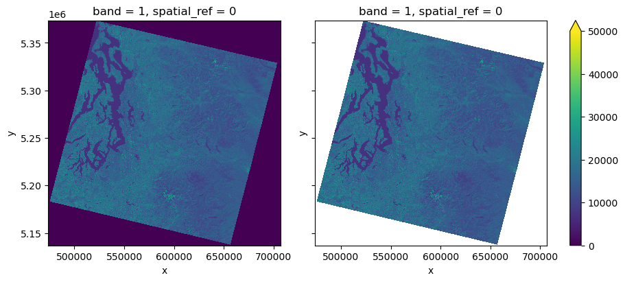
f,axs=plt.subplots(1,2, figsize=(9,4),sharey=True, layout='constrained')

nir_august_unmasked_da.plot.imshow(ax=axs[0],vmin=0,vmax=50000,add_colorbar=False)
nir_august_da.plot.imshow(ax=axs[1],vmin=0,vmax=50000)
<matplotlib.image.AxesImage at 0x7efc44232870>
nir_august_unmasked_da = None
Written response: Based on your observations, describe how rasterio and rioxarray handle masking differently. Based on only this insight, give an example of a case in which you might prefer to use rasterio over rioxarray.#
Hint: think about dtype
STUDENT WRITTEN RESPONSE HERE
Let’s proceed with using rioxarray for the remainder of the lab. We can use the rio accessor on an xarray DataArray (or Dataset) once we’ve imported rioxarray. The rio accessor allows us to use rioxarray’s functionalities. You can check out a list of rioxarray’s functions and the properties you can access from the rio accessor here.#
Inspect and print the following raster metadata using the xarray rio accessor… shape, height, width, nodata value, encoded nodata value, number of bands, CRS, resolution, extent, and transform. Try to print things neatly if you can using f strings.#
nir_august_da
<xarray.DataArray (y: 7891, x: 7771)> Size: 245MB
array([[nan, nan, nan, ..., nan, nan, nan],
       [nan, nan, nan, ..., nan, nan, nan],
       [nan, nan, nan, ..., nan, nan, nan],
       ...,
       [nan, nan, nan, ..., nan, nan, nan],
       [nan, nan, nan, ..., nan, nan, nan],
       [nan, nan, nan, ..., nan, nan, nan]], dtype=float32)
Coordinates:
    band         int64 8B 1
  * x            (x) float64 62kB 4.737e+05 4.737e+05 ... 7.068e+05 7.068e+05
  * y            (y) float64 63kB 5.374e+06 5.374e+06 ... 5.137e+06 5.137e+06
    spatial_ref  int64 8B 0
Attributes:
    AREA_OR_POINT:  Point
    scale_factor:   1.0
add_offset: 0.0# some examples...
# # nir_august_da.rio.shape
# nir_august_da.rio.crs
# STUDENT CODE HERE
Raster shape: (7891, 7771)
Raster height: 7891
Raster width: 7771
Raster nodata value: nan
Raster encoded nodata value: 0.0
Raster number of bands: 1
Raster CRS: EPSG:32610
Raster resolution: (30.0, -30.0)
Raster extent: (473685.0, 5136885.0, 706815.0, 5373615.0)
Raster transform:
| 30.00, 0.00, 473685.00|
| 0.00,-30.00, 5373615.00|
| 0.00, 0.00, 1.00|
What is the value of the right bound?#
Hint: The .rio.bounds() method returns a tuple with bounds formatted (left, bottom, right, top)
# STUDENT CODE HERE
Now we’ll open the red band for August with rioxarray, using masked=True and overview_level=2.#
red_august_da = rxr.open_rasterio(red_august_fn,masked=True,overview_level=2).squeeze()
red_august_da
<xarray.DataArray (y: 987, x: 972)> Size: 4MB
[959364 values with dtype=float32]
Coordinates:
band int64 8B 1
* x (x) float64 8kB 4.738e+05 4.74e+05 ... 7.065e+05 7.067e+05
* y (y) float64 8kB 5.373e+06 5.373e+06 ... 5.137e+06 5.137e+06
spatial_ref int64 8B 0
Attributes:
AREA_OR_POINT: Point
scale_factor: 1.0
add_offset: 0.0Written response: What did setting overview_level=2 do?#
STUDENT WRITTEN RESPONSE HERE
Make a figure with two subplots. On the left, plot the raster using the underlying numpy array. On the right, plot the raster using xarray DataArray’s built in .plot.imshow() functionality. Use a gray colormap with the same vmin and vmax for both, and please include a title on each.#
Hint: Remember, we can access an xarray DataArray’s underlying numpy array with .values
# STUDENT CODE HERE
red_august_da = None
Written response: Why does the Landsat-8 image appear rotated relative to the axes?#
STUDENT WRITTEN RESPONSE HERE
Written response: What is different about the two axes? We know the dimensions of the two arrays are the same, so what does this tell us about xarray DataArray coordinates? Feel free to inspect the xarray DataArray for clues.#
Hint: Think about pixel coordinates and projected coordinates
STUDENT WRITTEN RESPONSE HERE
Part 2: Converting to geophysical variables (3 pts)#
The values we’ve seen so far do not reflect geophysical variables! In order to convert from the digital number (DN) representation to surface reflectance (unitless 0.0-1.0) or surface temperature (K), we have to multiply by a scale factor and add an offset. Check out the download demo for more details.
First, let’s open the thermal infrared band with masked=False and overview=0…#
tir_august_da = rxr.open_rasterio(tir_august_fn,masked=False,overview_level=0).squeeze()
tir_august_da
<xarray.DataArray (y: 3946, x: 3886)> Size: 31MB
[15334156 values with dtype=uint16]
Coordinates:
band int64 8B 1
* x (x) float64 31kB 4.737e+05 4.738e+05 ... 7.067e+05 7.068e+05
* y (y) float64 32kB 5.374e+06 5.374e+06 ... 5.137e+06 5.137e+06
spatial_ref int64 8B 0
Attributes:
AREA_OR_POINT: Point
_FillValue: 0
scale_factor: 1.0
add_offset: 0.0Make a figure with a plot of the thermal infrared image on the left, and its corresponding histogram on the right.#
Hint: You can create a histogram with the xarray DataArray’s built-in .plot.hist()
# STUDENT CODE HERE
Written response: Why do you see a spike at 0 in the histogram?#
STUDENT WRITTEN RESPONSE HERE
Try making the previous figure again, this time loading with masked=True#
# STUDENT CODE HERE
# STUDENT CODE HERE
These values still don’t look very interpretable. Let’s convert them to degrees C.#
Hint: ST stands for surface temperature and SR stands for surface reflectance. Once you convert ST, be mindful this will be in degrees Kelvin. For better interpretability, please convert this to degrees Celsius.
#These are the standard scale and offset values
#SR 0.0000275 + -0.2
sr_scale = 0.0000275
sr_offset = -0.2
#ST 0.00341802 + 149.0
st_scale = 0.00341802
st_offset = 149.0
# STUDENT CODE HERE
<xarray.DataArray (y: 3946, x: 3886)> Size: 61MB
array([[nan, nan, nan, ..., nan, nan, nan],
       [nan, nan, nan, ..., nan, nan, nan],
       [nan, nan, nan, ..., nan, nan, nan],
       ...,
       [nan, nan, nan, ..., nan, nan, nan],
       [nan, nan, nan, ..., nan, nan, nan],
       [nan, nan, nan, ..., nan, nan, nan]], dtype=float32)
Coordinates:
band int64 8B 1
* x (x) float64 31kB 4.737e+05 4.738e+05 ... 7.067e+05 7.068e+05
* y (y) float64 32kB 5.374e+06 5.374e+06 ... 5.137e+06 5.137e+06
spatial_ref int64 8B 0Calculate the min and max surface temperature values, and the 2nd and 98th percentile of surface temperature values.#
Hint: You can use numpy functions on your xarray DataArray or the underlying numpy array. You can also use built-in xarray DataArray methods. Check out the np.nanpercentile or the built-in xarray DatArray .quantile method.
# STUDENT CODE HERE
Minimum temperature: -1.16°C
Maximum temperature: 99.85°C
# STUDENT CODE HERE
2nd percentile: 15.29°C
98th percentile: 39.24°C
Written response: We loaded this surface temperature raster in using its first overview (overview_level=0), effictively making the image coarser by a factor of two. Do you think the minimum, maximum, and percentile surface temperature values we calculated are the same as they would be in the full resolution image? How might this inform your future use of overviews?#
STUDENT WRITTEN RESPONSE HERE
With your updated surface temperature values, please make a final figure with pixel values on the left and the histogram on the right. Try using the inferno colormap, and set vmin=0 and vmax=40. Please also draw vertical lines for the 2nd and 98th percentile on the histogram.#
# STUDENT CODE HERE
Written response: Do the values make sense for August? Based on your image, where are the temperatures generally warmest? Coldest?#
STUDENT WRITTEN RESPONSE HERE
Part 3: Raster transform (2 pts)#
Written response: Inspect the transform property. In your own words, what does this represent? How would it be used mathematically?#
transform = tir_august_da.rio.transform()
transform
Affine(59.99227997941328, 0.0, 473685.0,
       0.0, -59.99239736441966, 5373615.0)
STUDENT WRITTEN RESPONSE HERE
Use the transform to convert the raster’s corner pixel coordinates to projected coordinates.#
Hint: After you calculate the projected coordinates of the corners, try using .rio.bounds() to see if your answer make sense in the context of this raster’s bounds
upper_left_pixel = (0,0)
lower_left_pixel = (0,tir_august_da.rio.height)
upper_right_pixel = (tir_august_da.rio.width,0)
lower_right_pixel = (tir_august_da.rio.width,tir_august_da.rio.height)

print(f'Upper left pixel: {upper_left_pixel}')
print(f'Lower left pixel: {lower_left_pixel}')
print(f'Upper right pixel: {upper_right_pixel}')
print(f'Lower right pixel: {lower_right_pixel}')
Upper left pixel: (0, 0)
Lower left pixel: (0, 3946)
Upper right pixel: (3886, 0)
Lower right pixel: (3886, 3946)
# STUDENT CODE HERE
Upper left projected: (473685.0, 5373615.0)
Lower left projected: (473685.0, 5136885.0)
Upper right projected: (706815.0, 5373615.0)
Lower right projected: (706815.0, 5136885.0)
# STUDENT CODE HERE
(473685.0, 5136885.0, 706815.0, 5373615.0)
Use the corner projected coordinates to compute the total dimensions of the raster in km.#
Print your answer with an f string with a format similar to Total height: height km, total width: width km
# STUDENT CODE HERE
Part 4: Raster windows (1 pts)#
Often times we only want to work with or view a small subset of a raster. This is helpful for many reasons, but will be especially helpful for us because a smaller raster will take up less RAM, and we are quite memory constrained on the jupyterhub. Using a smaller subset of the data is also great practice for prototyping new workflows, and makes analysis of larger-than-memory datasets possible.
In a pre-rioxarray world, you often had two choices for selecting subsets of data in python. If your raster was a numpy array, you could use simple array slicing to select a window, but that required reading in the entire numpy array beforehand. Rasterio’s rasterio.windows.Window functionality allowed for windowed reading of rasters, only loading into memory the portion of the raster you were interested in. All you have to do is pass a window object while reading, like src.read(band, window=window, masked=True). If you use rasterio, windowed reads are the way to go–check out the rasterio demo notebook for an example.
However, rioxarray (and xarray more broadly) does what’s called a “lazy load”. There’s some nuance here, especially as it relates to similar concepts we’ll explore with a package called dask in later modules, but we’ll skip most of the complexity for now. At its simplist, lazy loading allows us to view and interact with the metadata of a raster without the full data being loaded into memory.
Lazy loading, along with xarray’s intuitive .sel and .isel selection methods, will enable us to get the benefits of windowed reads with greater flexibility and more intuitive syntax.
To select a window in projected coordinates (coordinate labels), use:
da.sel(x=slice(x_min,x_max),y=slice(y_max,y_min))
and for pixel coordinates (integer array indicies), use:
da.isel(x=slice(x_min,x_max),y=slice(y_min,y_max))
notice how the slicing flips for y due to pixel coordinates increasing from the top of the raster to the bottom of the raster.
Let’s try extracting a window around Mt. Rainier using both methods#
This time we’ll open the thermal infrared image again, with masking, but the full resolution raster
tir_august_da = rxr.open_rasterio(tir_august_fn,masked=True).squeeze()
tir_august_da
<xarray.DataArray (y: 7891, x: 7771)> Size: 245MB
[61320961 values with dtype=float32]
Coordinates:
    band         int64 8B 1
  * x            (x) float64 62kB 4.737e+05 4.737e+05 ... 7.068e+05 7.068e+05
  * y            (y) float64 63kB 5.374e+06 5.374e+06 ... 5.137e+06 5.137e+06
    spatial_ref  int64 8B 0
Attributes:
    AREA_OR_POINT:  Point
    scale_factor:   1.0
add_offset: 0.0Use .sel() and .isel() to select a window around Mt. Rainier. Convert to surface temperature in degrees C, and then plot these next to each other.#
Hint: For the window, you can use [581685.0, 5174895.0, 612405.0, 5205615.0] for projected coordinates, and [3600, 6624, 4624, 5600] for pixel coordinates. Remember when y slicing is reversed :)
# STUDENT CODE HERE
<xarray.DataArray (y: 1024, x: 1024)> Size: 4MB
[1048576 values with dtype=float32]
Coordinates:
    band         int64 8B 1
  * x            (x) float64 8kB 5.817e+05 5.817e+05 ... 6.124e+05 6.124e+05
  * y            (y) float64 8kB 5.206e+06 5.206e+06 ... 5.175e+06 5.175e+06
    spatial_ref  int64 8B 0
Attributes:
    AREA_OR_POINT:  Point
    scale_factor:   1.0
add_offset: 0.0# STUDENT CODE HERE
<xarray.DataArray (y: 1024, x: 1024)> Size: 4MB
[1048576 values with dtype=float32]
Coordinates:
    band         int64 8B 1
  * x            (x) float64 8kB 5.817e+05 5.817e+05 ... 6.124e+05 6.124e+05
  * y            (y) float64 8kB 5.206e+06 5.206e+06 ... 5.175e+06 5.175e+06
    spatial_ref  int64 8B 0
Attributes:
    AREA_OR_POINT:  Point
    scale_factor:   1.0
add_offset: 0.0tir_august_subset_geo_da = st_scale*tir_august_subset_geo_da+st_offset
tir_august_subset_geo_da = tir_august_subset_geo_da-273.15
tir_august_subset_pix_da = st_scale*tir_august_subset_pix_da+st_offset
tir_august_subset_pix_da = tir_august_subset_pix_da-273.15
# STUDENT CODE HERE
tir_august_subset_pix_da = None
tir_august_subset_da = tir_august_subset_geo_da
tir_august_subset_geo_da = None
Part 5: Raster sampling (1 pts)#
Previously, rasterio users would have to use src.xy and src.index to convert between pixel and projected coordinates. They would either need to convert to pixel coordinates to index into the numpy array, or they would have to use src.sample.
Rioxarray’s (xarray’s) .sel() and .isel() functionalities can be really helpful for raster sampling as well. Since .isel() selects based integer array coordinates, you can enter in pixel coordinates. .sel() selects based on coordinate labels, so you can enter projected coordinates. When selecting projected coordinates which are often float values, we’ll use method='nearest' since we likely won’t know the exact coordinate discretization.
To select a point based on projected coordinates:
da.sel(x=x_coord,y=y_coord,method="nearest")
and for pixel coordinates:
da.isel(x=x_coord,y=y_coord)
Given the following points to sample, print the surface temperature value at that point. Note that the first two points are in the projected coordinates, the third point is in pixel coordinates, and the fourth point is in latitude and longitude.#
Hint: We’ve defined a Transformer for you to convert the 4th point’s latitude and longitude to a point in this CRS. See the sampling section of the rioxarray demo for more help.
glacier_proj_point = (595949,5190623)
sun_facing_proj_point = (600000,5195620)
shaded_pixel_point = (539,264)
parking_lot_latlon_point = (-121.7354,46.7856)

transform_4326_point_to_raster_crs = pyproj.Transformer.from_crs("EPSG:4326",tir_august_subset_da.rio.crs,always_xy=True)
# STUDENT CODE HERE
print(f'Glacier pixel temperature: {glacier_value:.2f}°C')
print(f'Sun-facing pixel temperature: {sun_facing_value:.2f}°C')
print(f'Shaded pixel temperature: {shaded_pixel_value:.2f}°C')
print(f'Paradise parking lot pixel temperature: {parking_lot_value:.2f}°C')
Glacier pixel temperature: 0.83°C
Sun-facing pixel temperature: 41.75°C
Shaded pixel temperature: 18.97°C
Paradise parking lot pixel temperature: 32.61°C
Challenge question: Plot the four points on top of the surface temperature raster and add a scalebar (GS: Attempt required / UG: +1 pts)#
Hint: You will likely have to transform the shaded pixel point and parking lot point before plotting
# STUDENT CODE HERE
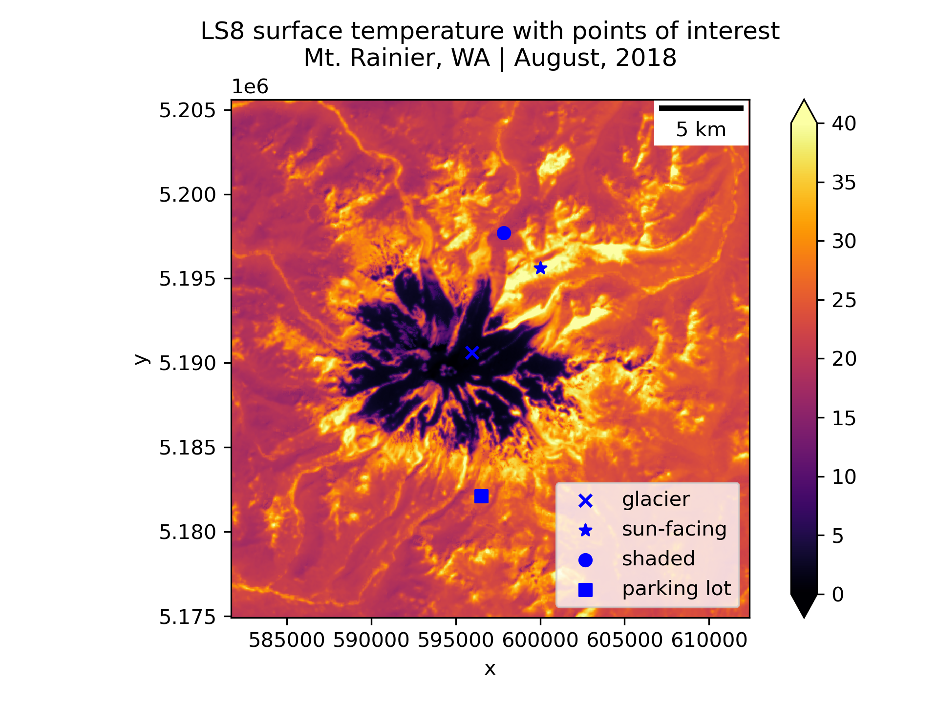
Written response: Do the temperatures seem reasonable for their respective locations?#
STUDENT WRITTEN RESPONSE HERE
Great work, you finished notebook 1! Move on to Notebook #2, but first…#
Save this notebook!
You can also do an add, commit, and push at this stage
Shut down the kernel to free RAM
Proceed to Notebook #2!