Lab 05 assignment (20 pts)#
UW Geospatial Data Analysis
CEE467/CEWA567
David Shean, Eric Gagliano, Quinn Brencher
Introduction#
Objectives#
Continue to explore GeoPandas functionality
Explore basic geometry operations (e.g., buffer, intersect, union)
Explore spatial filtering and spatial joins
Explore new visualization approaches (e.g., hexbin, interactive maps)
In order to cover some additional important vector concepts, let’s use a power plants dataset, and also explore some King County census data in tandem with some toxic release data.
Instructions#
For each question or task below, write some code in the empty cell and execute to preserve your output
If you are in the graduate section of the class, please complete the challenge questions
Work together, consult resources we’ve discussed, post on slack!
Remember, the lab assignment this week is broken into two notebooks!
Part 0: Prepare data#
!pip install -q censusdata
import matplotlib.pyplot as plt
import matplotlib.colors as colors
import numpy as np
import pandas as pd
import geopandas as gpd
from shapely.geometry import Point, Polygon
import xyzservices.providers as xyz
import os
import contextily as ctx
import censusdata
import seaborn as sns
import requests
import zipfile
import shutil
Load in the power plants data#
These data are a subset of a cool global power plant dataset:
Global Energy Observatory, Google, KTH Royal Institute of Technology in Stockholm, University of Groningen, World Resources Institute. 2018. Global Power Plant Database. Published on Resource Watch and Google Earth Engine; https://resourcewatch.org/ https://earthengine.google.com/
For details about this dataset, including a key to the column names, see https://developers.google.com/earth-engine/datasets/catalog/WRI_GPPD_power_plants#table-schema
Load the power plants geojson file into a GeoDataFrame and check the crs
# read in the data
pplant_fn = './data/conus_power_plants.geojson'
pplant_gdf = gpd.read_file(pplant_fn)
pplant_gdf.crs
<Geographic 2D CRS: EPSG:4326>
Name: WGS 84
Axis Info [ellipsoidal]:
- Lat[north]: Geodetic latitude (degree)
- Lon[east]: Geodetic longitude (degree)
Area of Use:
- name: World.
- bounds: (-180.0, -90.0, 180.0, 90.0)
Datum: World Geodetic System 1984 ensemble
- Ellipsoid: WGS 84
- Prime Meridian: Greenwich
# take a quick look
pplant_gdf.head()
| cap_year | capacitymw | comm_year | country | country_lg | fuel1 | fuel2 | fuel3 | fuel4 | gppd_idnr | ... | gwh_2014 | gwh_2015 | gwh_2016 | gwh_estimt | latitude | longitude | name | owner | source | geometry | |
|---|---|---|---|---|---|---|---|---|---|---|---|---|---|---|---|---|---|---|---|---|---|
| 0 | 0.0 | 149.0 | 1969.00000 | USA | United States of America | Gas | None | None | None | USA0001233 | ... | 0.0 | 0.0 | -0.209 | 613.166810 | 37.7328 | -99.9497 | Fort Dodge | Sunflower Electric Power Corp | U.S. Energy Information Administration | POINT (-99.9497 37.7328) |
| 1 | 0.0 | 730.2 | 2008.46946 | USA | United States of America | Gas | None | None | None | USA0056502 | ... | 0.0 | 0.0 | 333.957 | 3004.928891 | 38.4459 | -96.0652 | Emporia Energy Center | Westar Energy Inc | U.S. Energy Information Administration | POINT (-96.0652 38.4459) |
| 2 | 0.0 | 11.0 | 1962.00000 | USA | United States of America | Gas | None | None | None | USA0001332 | ... | 0.0 | 0.0 | 0.005 | 45.267348 | 37.2354 | -97.0110 | West 14th Street | City of Winfield - (KS) | U.S. Energy Information Administration | POINT (-97.011 37.2354) |
| 3 | 0.0 | 228.0 | 1957.50000 | USA | United States of America | Gas | None | None | None | USA0001242 | ... | 0.0 | 0.0 | 75.912 | 938.268676 | 37.5967 | -97.4136 | Murray Gill | Kansas Gas & Electric Co | U.S. Energy Information Administration | POINT (-97.4136 37.5967) |
| 4 | 0.0 | 43.7 | 1982.00000 | USA | United States of America | Gas | None | None | None | USA0050169 | ... | 0.0 | 0.0 | 0.000 | 179.834830 | 37.5813 | -97.4241 | Wichita Plant | Occidental Chemical Corporation | U.S. Energy Information Administration | POINT (-97.4241 37.5813) |
5 rows × 21 columns
Now we’ll read in the state polygons…#
states_url = 'http://eric.clst.org/assets/wiki/uploads/Stuff/gz_2010_us_040_00_5m.json'
states_gdf = gpd.read_file(states_url)
states_gdf
| GEO_ID | STATE | NAME | LSAD | CENSUSAREA | geometry | |
|---|---|---|---|---|---|---|
| 0 | 0400000US01 | 01 | Alabama | 50645.326 | MULTIPOLYGON (((-88.12466 30.28364, -88.08681 ... | |
| 1 | 0400000US02 | 02 | Alaska | 570640.950 | MULTIPOLYGON (((-166.10574 53.98861, -166.0752... | |
| 2 | 0400000US04 | 04 | Arizona | 113594.084 | POLYGON ((-112.53859 37.00067, -112.53454 37.0... | |
| 3 | 0400000US05 | 05 | Arkansas | 52035.477 | POLYGON ((-94.04296 33.01922, -94.04304 33.079... | |
| 4 | 0400000US06 | 06 | California | 155779.220 | MULTIPOLYGON (((-122.42144 37.86997, -122.4213... | |
| 5 | 0400000US08 | 08 | Colorado | 103641.888 | POLYGON ((-106.19055 40.99761, -106.06118 40.9... | |
| 6 | 0400000US09 | 09 | Connecticut | 4842.355 | POLYGON ((-71.79924 42.00806, -71.79792 41.935... | |
| 7 | 0400000US10 | 10 | Delaware | 1948.543 | MULTIPOLYGON (((-75.56493 39.58325, -75.57627 ... | |
| 8 | 0400000US11 | 11 | District of Columbia | 61.048 | POLYGON ((-77.0386 38.79151, -77.0389 38.80081... | |
| 9 | 0400000US12 | 12 | Florida | 53624.759 | MULTIPOLYGON (((-82.82158 27.96444, -82.8298 2... | |
| 10 | 0400000US13 | 13 | Georgia | 57513.485 | POLYGON ((-84.81048 34.98761, -84.80918 34.987... | |
| 11 | 0400000US15 | 15 | Hawaii | 6422.628 | MULTIPOLYGON (((-155.77823 20.24574, -155.7727... | |
| 12 | 0400000US16 | 16 | Idaho | 82643.117 | POLYGON ((-111.04416 43.02005, -111.04413 43.0... | |
| 13 | 0400000US17 | 17 | Illinois | 55518.930 | POLYGON ((-89.36603 42.50027, -89.36156 42.500... | |
| 14 | 0400000US18 | 18 | Indiana | 35826.109 | POLYGON ((-84.80248 40.52805, -84.80255 40.501... | |
| 15 | 0400000US19 | 19 | Iowa | 55857.130 | POLYGON ((-91.21771 43.50055, -91.21827 43.497... | |
| 16 | 0400000US20 | 20 | Kansas | 81758.717 | POLYGON ((-99.54112 36.99957, -99.55807 36.999... | |
| 17 | 0400000US21 | 21 | Kentucky | 39486.338 | MULTIPOLYGON (((-89.48511 36.49769, -89.49254 ... | |
| 18 | 0400000US22 | 22 | Louisiana | 43203.905 | MULTIPOLYGON (((-88.86507 29.75271, -88.88976 ... | |
| 19 | 0400000US23 | 23 | Maine | 30842.923 | MULTIPOLYGON (((-70.15259 43.74679, -70.15196 ... | |
| 20 | 0400000US24 | 24 | Maryland | 9707.241 | MULTIPOLYGON (((-76.04837 38.12055, -76.05681 ... | |
| 21 | 0400000US25 | 25 | Massachusetts | 7800.058 | MULTIPOLYGON (((-70.8274 41.60207, -70.82374 4... | |
| 22 | 0400000US26 | 26 | Michigan | 56538.901 | MULTIPOLYGON (((-85.82596 45.4043, -85.83352 4... | |
| 23 | 0400000US27 | 27 | Minnesota | 79626.743 | POLYGON ((-92.20469 46.70404, -92.20569 46.702... | |
| 24 | 0400000US28 | 28 | Mississippi | 46923.274 | MULTIPOLYGON (((-89.09562 30.23177, -89.07726 ... | |
| 25 | 0400000US29 | 29 | Missouri | 68741.522 | POLYGON ((-89.54501 36.33681, -89.56044 36.337... | |
| 26 | 0400000US30 | 30 | Montana | 145545.801 | POLYGON ((-105.0384 45.00034, -105.07661 45.00... | |
| 27 | 0400000US31 | 31 | Nebraska | 76824.171 | POLYGON ((-104.05325 41.00141, -104.05316 41.0... | |
| 28 | 0400000US32 | 32 | Nevada | 109781.180 | POLYGON ((-114.04214 40.99993, -114.04318 40.7... | |
| 29 | 0400000US33 | 33 | New Hampshire | 8952.651 | POLYGON ((-72.4521 43.16141, -72.45187 43.1701... | |
| 30 | 0400000US34 | 34 | New Jersey | 7354.220 | POLYGON ((-75.21088 39.86571, -75.21042 39.865... | |
| 31 | 0400000US35 | 35 | New Mexico | 121298.148 | POLYGON ((-105.998 32.00233, -106.09976 32.002... | |
| 32 | 0400000US36 | 36 | New York | 47126.399 | MULTIPOLYGON (((-74.04086 40.70012, -74.04002 ... | |
| 33 | 0400000US37 | 37 | North Carolina | 48617.905 | MULTIPOLYGON (((-75.75376 35.19961, -75.74522 ... | |
| 34 | 0400000US38 | 38 | North Dakota | 69000.798 | POLYGON ((-98.72438 45.93869, -98.90443 45.939... | |
| 35 | 0400000US39 | 39 | Ohio | 40860.694 | MULTIPOLYGON (((-82.83512 41.70897, -82.82572 ... | |
| 36 | 0400000US40 | 40 | Oklahoma | 68594.921 | POLYGON ((-96.94461 33.94922, -96.95231 33.944... | |
| 37 | 0400000US41 | 41 | Oregon | 95988.013 | POLYGON ((-121.92224 45.64908, -121.90827 45.6... | |
| 38 | 0400000US42 | 42 | Pennsylvania | 44742.703 | POLYGON ((-79.91617 39.72089, -80.07595 39.721... | |
| 39 | 0400000US44 | 44 | Rhode Island | 1033.814 | MULTIPOLYGON (((-71.38359 41.46478, -71.38928 ... | |
| 40 | 0400000US45 | 45 | South Carolina | 30060.696 | POLYGON ((-79.29075 33.11005, -79.29159 33.109... | |
| 41 | 0400000US46 | 46 | South Dakota | 75811.000 | POLYGON ((-104.05449 44.18038, -104.05539 44.2... | |
| 42 | 0400000US47 | 47 | Tennessee | 41234.896 | POLYGON ((-83.47211 36.59728, -83.3749 36.5973... | |
| 43 | 0400000US48 | 48 | Texas | 261231.711 | MULTIPOLYGON (((-97.13436 27.89633, -97.1336 2... | |
| 44 | 0400000US49 | 49 | Utah | 82169.620 | POLYGON ((-111.04655 41.25172, -111.04672 40.9... | |
| 45 | 0400000US50 | 50 | Vermont | 9216.657 | POLYGON ((-72.4338 43.233, -72.43447 43.23043,... | |
| 46 | 0400000US51 | 51 | Virginia | 39490.086 | MULTIPOLYGON (((-75.97361 37.83582, -75.9717 3... | |
| 47 | 0400000US53 | 53 | Washington | 66455.521 | MULTIPOLYGON (((-122.51954 48.28831, -122.5227... | |
| 48 | 0400000US54 | 54 | West Virginia | 24038.210 | POLYGON ((-80.07595 39.72135, -79.91617 39.720... | |
| 49 | 0400000US55 | 55 | Wisconsin | 54157.805 | MULTIPOLYGON (((-90.40331 47.02669, -90.40332 ... | |
| 50 | 0400000US56 | 56 | Wyoming | 97093.141 | POLYGON ((-110.04848 40.99756, -110.12164 40.9... | |
| 51 | 0400000US72 | 72 | Puerto Rico | 3423.775 | MULTIPOLYGON (((-65.3277 18.29584, -65.33745 1... |
Limit states_gdf to the lower 48#
We want to filter out Alaska, Puerto Rico, and Hawaii from this dataset
One possible approach would be to use boolean indexing on states_gdf, creating an index where states_gdf[‘NAME’] contains Alaska, Puero Rico, and Hawaii
Then you could index back into states_gdf where your index is False
Hint: Check out the .isin() function
# STUDENT CODE HERE
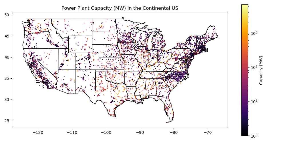
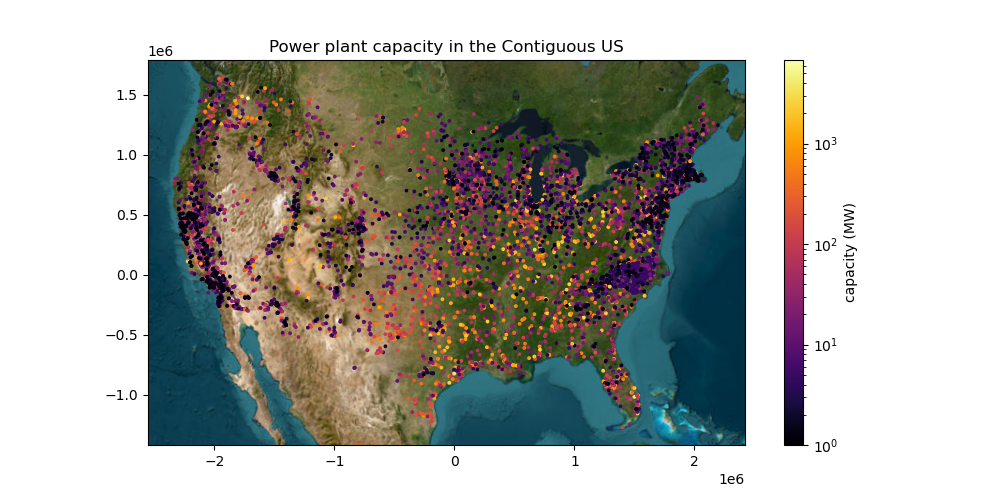
Create a quick plot of power plant capacity overlayed on top of the state polygons to verify everything looks good#
Can re-use plotting code near the end of Lab04
If plotting a variable that is highly skewed to one side, consider passing
norm=colors.LogNorm()to yourplot()function to create a logarithmic colorbar.Note that here we’re plotting in WGS84, not a projected coordinate system. This will result in some distortions!
# STUDENT CODE HERE
Extract the MultiPolygon geometry object for Washington from your reprojected states GeoDataFrame#
Use the state ‘NAME’ value to isolate the approprate GeoDataFrame record for Washington to create
wa_gdf
# STUDENT CODE HERE
Part 1: Geometric Operations for power plant points (4 pts)#
Clip the power plant points to Washington state polygon#
You could do this in two steps:
Identify records from the power plants GeoDataFrame that
intersectsthe WA state geometryExtract those records and store in a new GeoDataFrame
# STUDENT CODE HERE
Define an azimuthal equidistant projection for Washington State#
We’re going to do calculations of distance in this section, so we need to use a projection that preserves distance
Let’s quickly define a custom Azimuthal Equidistant projection for our power plant points and polgyons
ae_proj_str = f'+proj=aeqd +lat_0={wa_gdf.iloc[0].geometry.centroid.y:.2f} +lon_0={wa_gdf.iloc[0].geometry.centroid.x:.2f} +datum=WGS84 +units=m +no_defs'
pplant_gdf_wa = pplant_gdf_wa.to_crs(ae_proj_str)
wa_gdf = wa_gdf.to_crs(ae_proj_str)
Compute some statistics for the WA state power plants#
How many power plants are in WA state?
What is median
capacitymwcapacity of WA state power plants in megawatts?
# STUDENT CODE HERE
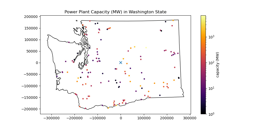
There are 138 power plants in Washington state.
# STUDENT CODE HERE
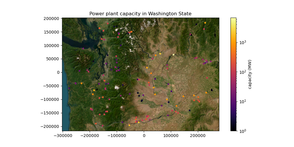
Plot the resulting points#
Add the WA polygon outline
Note that you don’t need/want to use the Polygon Geometry object here. Remember, you have a GeoDataFrame containing just the WA geometry. And you know how to plot GeoDataFrames.
Add the WA state centroid you calculated earlier using a distinct marker style (e.g.,
'*'or'x')Can use simple matplotlib
plotwith the coordinates, or can usewa_gdf.centroid.plot()
As above, consider passing
norm=colors.LogNorm()to yourplot()function to create a logarithmic colorbar.
# STUDENT CODE HERE
Find the distance from the power plants to the WA state centroid#
See the GeoDataFrame
distancefunctionCreate a plot showing this distance for each power plant point.
c = wa_gdf.iloc[0].geometry.centroid
# STUDENT CODE HERE
# STUDENT CODE HERE
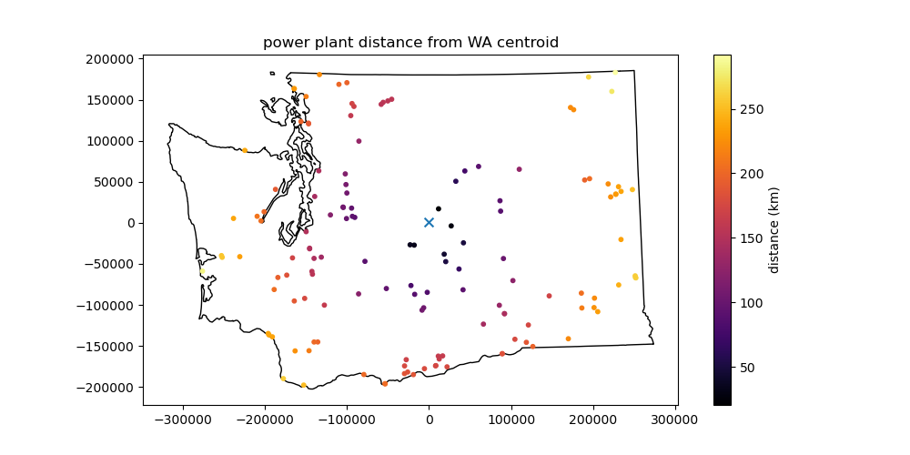
What is the distance between this point (point closest to the centroid) and the centroid in km?#
# STUDENT CODE HERE
What is the capacitymw value of this point?#
For this, we need to isolate the original GeoDataFrame record corresponding to the minimum distance
We talked about
argminorargmaxfor NumPy arrays. For a DataFrame, we want to use theidxmin()method on the column or DataSeries containing the distance values, which should give us the index value:https://pandas.pydata.org/docs/reference/api/pandas.DataFrame.idxmin.html
Can then use the index value to locate the corresponding record in the GeoDataFrame with standard Pandas indexing: https://pandas.pydata.org/docs/user_guide/indexing.html
# STUDENT CODE HERE
# STUDENT CODE HERE
# STUDENT CODE HERE
The closest power plant to the centroid of Washington state has a capacity of 1299.6 MW.
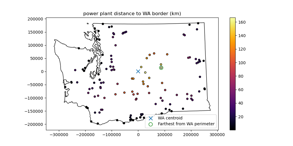
Challenge Question (GS required/UG +0.5): Which power plant is farthest from the WA state perimeter?#
Note that this is different than the above calcuations for point to point distance, you’re looking for point to polyline distance
What is the distance in km?
This should be pretty straightforward, combining elements from the above questions/demo
This kind of calculation can be useful to consider distance from the coast and climatology (temperature, precipitation and other environmental variables)
# STUDENT CODE HERE
# STUDENT CODE HERE
# STUDENT CODE HERE
Part 2: Aggregate power plants for state polygons and compute capacitymw statistics (3 pts)#
OK, we computed some stats for power plants within WA state. Now let’s find the power plants that intersect each state polygon.
Objectives:
Compute the total number of power plants and total
capacitymwenergy generation capacity for each stateGenerate choropleth maps for both
One approach would be to loop through each state polygon, and do an intersection operation like we did for WA state above. But this is inefficient, and doesn’t scale well. It is much more efficient to do a spatial join between the power plant points and the polygons with the intersection operator, then groupby and aggregate to compute the relevant statistics for each state.
You may have learned how to perform a join or spatial join in a GIS class, perhaps using ArcMap or QGIS here. Luckily, GeoPandas has you covered.
First, let’s define an Albers Equal Area projection for our data#
We’re going to be doing area-based calculations in this section, so we need to use a projection that preserves area
We need to project both the power plant points and the state polygons
# get extent and center coordinates
pplant_extent = pplant_gdf.total_bounds
pplant_center_x = (pplant_extent[0] + pplant_extent[2])/2
pplant_center_y = (pplant_extent[3] + pplant_extent[1])/2
# define proj string
aea_proj_str = f'+proj=aea +lat_1={pplant_extent[1]:.2f} +lat_2={pplant_extent[3]:.2f} +lat_0={pplant_center_y:.2f} +lon_0={pplant_center_x:.2f}'
# reproject
pplant_gdf_aea = pplant_gdf.to_crs(aea_proj_str)
states_gdf_aea = states_gdf.to_crs(aea_proj_str)
Now we can get rolling with analysis!
Start with a spatial join between the power plant points and state polygons#
Start by reviewing the Spatial Join documentation
Use the geopandas
sjoinmethod
Let’s extract the columns that matter to us#
Since we only care about
capacitymwvalues here let’s create some smaller GeoDataFrames:Extract the
['capacitymw', 'geometry']columns from the power plant GeoDataFrameExtract the
['NAME', 'geometry']columns from the states GeoDataFrame
pplant_gdf_aea_lite = pplant_gdf_aea[['capacitymw', 'geometry']]
states_gdf_aea_lite = states_gdf_aea[['NAME','geometry']]
Now try a spatial join between these two#
Use the power plant points as the “left” GeoDataFrame and the States as the “right” GeoDataFrame
Start by using default options (
op='intersects', how='inner')Note the output geometry type and columns
# STUDENT CODE HERE
| capacitymw | geometry | index_right | NAME | |
|---|---|---|---|---|
| 0 | 149.0 | POINT (-373798.752 116463.932) | 16 | Kansas |
| 1 | 730.2 | POINT (-38844.692 189244.381) | 16 | Kansas |
| 2 | 11.0 | POINT (-121518.346 52569.772) | 16 | Kansas |
| 3 | 228.0 | POINT (-155679.348 94157.393) | 16 | Kansas |
| 4 | 43.7 | POINT (-156617.964 92425.8) | 16 | Kansas |
| ... | ... | ... | ... | ... |
| 7863 | 1.3 | POINT (1763173.316 1010517.952) | 45 | Vermont |
| 7864 | 1.8 | POINT (1828872.636 991070.108) | 45 | Vermont |
| 7865 | 1.8 | POINT (1783973.835 1092752.901) | 45 | Vermont |
| 7866 | 1.8 | POINT (1787741.825 1101022.7) | 45 | Vermont |
| 7867 | 1.8 | POINT (1812915.624 1010086.014) | 45 | Vermont |
7868 rows × 4 columns
Now reverse the order of the two input GeoDataFrames#
Use default options again
# STUDENT CODE HERE
Which one makes more sense?#
Remember, we’re trying to add a State name to each power plant
You’ll need to decide which one to use moving forward
# STUDENT CODE HERE
Confidence check#
Run a
headon our new GeoDataFrameFor each power plant point, there should be a new column with the corresponding state NAME
# STUDENT CODE HERE
| capacitymw | geometry | index_right | NAME | |
|---|---|---|---|---|
| 0 | 149.0 | POINT (-373798.752 116463.932) | 16 | Kansas |
| 1 | 730.2 | POINT (-38844.692 189244.381) | 16 | Kansas |
| 2 | 11.0 | POINT (-121518.346 52569.772) | 16 | Kansas |
| 3 | 228.0 | POINT (-155679.348 94157.393) | 16 | Kansas |
| 4 | 43.7 | POINT (-156617.964 92425.8) | 16 | Kansas |
Now aggregate by state NAME#
Note: the GeoPandas doc example uses a
dissolveoperation here, which is a wrapper around thegroupbyandaggPandas functionshttps://geopandas.org/en/stable/docs/user_guide/aggregation_with_dissolve.html
But look at the geometry column for the points in your GeoDataFrame. The
dissolveis going to compute the union for the points in each state and return aMultiPointGeometry for each state, which we don’t really want/need. It will also take longer to run.Instead, let’s try a
groupbyoperation for theNAMEcolumn, and thenaggwith a list of functions we care about:['count', 'sum'](statistics for point count and mean point elevation for each state)We did this in Lab02!
# STUDENT CODE HERE
| count | sum | |
|---|---|---|
| NAME | ||
| Alabama | 71 | 31451.9 |
| Arizona | 121 | 32991.9 |
| Arkansas | 56 | 16341.8 |
| California | 1273 | 82100.4 |
| Colorado | 163 | 17838.5 |
| Connecticut | 94 | 7489.1 |
| Delaware | 25 | 3628.3 |
| District of Columbia | 2 | 24.9 |
| Florida | 148 | 66705.4 |
| Georgia | 157 | 39580.0 |
| Idaho | 135 | 5672.2 |
| Illinois | 204 | 50908.7 |
| Indiana | 141 | 28438.7 |
| Iowa | 228 | 18334.7 |
| Kansas | 131 | 16526.4 |
| Kentucky | 47 | 24066.4 |
| Louisiana | 83 | 28351.8 |
| Maine | 101 | 5211.7 |
| Maryland | 93 | 13710.0 |
| Massachusetts | 299 | 14769.4 |
| Michigan | 222 | 29868.9 |
| Minnesota | 304 | 17829.1 |
| Mississippi | 41 | 18073.9 |
| Missouri | 119 | 23758.3 |
| Montana | 51 | 6446.7 |
| Nebraska | 101 | 9186.8 |
| Nevada | 77 | 12213.3 |
| New Hampshire | 65 | 4699.7 |
| New Jersey | 257 | 20737.8 |
| New Mexico | 95 | 9264.8 |
| New York | 384 | 42593.2 |
| North Carolina | 552 | 35402.8 |
| North Dakota | 54 | 8334.6 |
| Ohio | 156 | 31533.0 |
| Oklahoma | 100 | 28318.4 |
| Oregon | 151 | 11397.9 |
| Pennsylvania | 212 | 48174.7 |
| Rhode Island | 27 | 2063.9 |
| South Carolina | 97 | 24738.1 |
| South Dakota | 34 | 4390.3 |
| Tennessee | 64 | 24029.0 |
| Texas | 404 | 128609.5 |
| Utah | 100 | 9798.3 |
| Vermont | 85 | 647.0 |
| Virginia | 135 | 28348.7 |
| Washington | 138 | 36879.8 |
| West Virginia | 35 | 16041.4 |
| Wisconsin | 173 | 17793.4 |
| Wyoming | 63 | 9480.2 |
Confidence check#
That groupby and agg should be pretty fast (~1-2 seconds)
Check the
type()of the outputSince
groupbyandaggare Pandas operation, you should now have a new PandasDataFrame(not a GeoPandasGeoDataFrame) with index of state names and columns forcountandmeanvalues in each state
# STUDENT CODE HERE
Part 3: Plots! (2 pts)#
How are we going to visualize these data?
We have
countpower plant points andsumof power plant capacity for each state! Objective #1 complete!We now want to visualize these values, but we lost our state Polygon/MultiPolygon Geometry along the way
No problem, we can combine our DataFrame with the original State GeoDataFrame
Can use
mergeto do an attribute join on the shared state'NAME'index for the twoTake a moment to review the
my_agg_df.merge?optionsIn this case, we have a common
NAMEfield, so we can use theon='NAME'here for attribute join
Careful about the order of the two inputs here (state GeoDataFrame and the DataFrame with your stats) - you want to preserve the index and geometry of the GeoDataFrame, adding the
countandmeancolumns.If you get it right, you should be able to
plot()the GeoPandas GeoDataFrame and get a map. If you got it backwards, the output ofplot()will be a line plot for the regular Pandas DataFrame
Combine states_gdf_aea_lite and pplant_gdf_aea_states_agg#
# STUDENT CODE HERE
| NAME | geometry | count | sum | |
|---|---|---|---|---|
| 0 | Alabama | MULTIPOLYGON (((708732.822 -707811.735, 712514... | 71 | 31451.9 |
| 1 | Arizona | POLYGON ((-1465661.328 152092.001, -1465314.16... | 121 | 32991.9 |
| 2 | Arkansas | POLYGON ((143568.999 -425106.846, 143453.305 -... | 56 | 16341.8 |
| 3 | California | MULTIPOLYGON (((-2277167.082 437548.205, -2277... | 1273 | 82100.4 |
| 4 | Colorado | POLYGON ((-869898.203 525860.898, -859309.622 ... | 163 | 17838.5 |
| 5 | Connecticut | POLYGON ((1914586.875 827355.12, 1916674.15 81... | 94 | 7489.1 |
| 6 | Delaware | MULTIPOLYGON (((1672374.733 490114.235, 167132... | 25 | 3628.3 |
| 7 | District of Columbia | POLYGON ((1567915.217 377568.875, 1567691.059 ... | 2 | 24.9 |
| 8 | Florida | MULTIPOLYGON (((1242485.092 -913944.857, 12416... | 148 | 66705.4 |
| 9 | Georgia | POLYGON ((962929.008 -150182.712, 963044.303 -... | 157 | 39580.0 |
| 10 | Idaho | POLYGON ((-1230181.552 805125.905, -1230203.4 ... | 135 | 5672.2 |
| 11 | Illinois | POLYGON ((503155.34 665167.903, 503516.948 665... | 204 | 50908.7 |
| 12 | Indiana | POLYGON ((894352.421 474951.802, 894675.136 47... | 141 | 28438.7 |
| 13 | Iowa | POLYGON ((348987.571 770124.612, 348959.631 76... | 228 | 18334.7 |
| 14 | Kansas | POLYGON ((-341967.525 31793.248, -343441.586 3... | 131 | 16526.4 |
| 15 | Kentucky | MULTIPOLYGON (((536161.774 -15266.298, 535511.... | 47 | 24066.4 |
| 16 | Louisiana | MULTIPOLYGON (((642856.893 -772479.666, 640773... | 83 | 28351.8 |
| 17 | Maine | MULTIPOLYGON (((1993500.901 1050797.037, 19934... | 101 | 5211.7 |
| 18 | Maryland | MULTIPOLYGON (((1665553.015 319169.587, 166474... | 93 | 13710.0 |
| 19 | Massachusetts | MULTIPOLYGON (((2002613.155 802194.458, 200300... | 299 | 14769.4 |
| 20 | Michigan | MULTIPOLYGON (((754921.168 1014852.429, 754632... | 222 | 29868.9 |
| 21 | Minnesota | POLYGON ((258053.196 1127649.709, 257983.22 11... | 304 | 17829.1 |
| 22 | Mississippi | MULTIPOLYGON (((617333.202 -720210.395, 619071... | 41 | 18073.9 |
| 23 | Missouri | POLYGON ((532055.49 -33817.124, 530696.779 -33... | 119 | 23758.3 |
| 24 | Montana | POLYGON ((-731942.509 966869.411, -734898.94 9... | 51 | 6446.7 |
| 25 | Nebraska | POLYGON ((-694630.265 509210.448, -694472.302 ... | 101 | 9186.8 |
| 26 | Nevada | POLYGON ((-1509379.882 621585.357, -1514309.94... | 77 | 12213.3 |
| 27 | New Hampshire | POLYGON ((1832486.548 941701.831, 1832272.334 ... | 65 | 4699.7 |
| 28 | New Jersey | POLYGON ((1694855.025 527587.343, 1694887.162 ... | 257 | 20737.8 |
| 29 | New Mexico | POLYGON ((-962156.637 -490075.176, -971543.292... | 95 | 9264.8 |
| 30 | New York | MULTIPOLYGON (((1769835.568 640821.672, 176988... | 384 | 42593.2 |
| 31 | North Carolina | MULTIPOLYGON (((1757076.83 -505.517, 1757744.4... | 552 | 35402.8 |
| 32 | North Dakota | POLYGON ((-238747.793 1041014.554, -252542.498... | 54 | 8334.6 |
| 33 | Ohio | MULTIPOLYGON (((1038876.036 627347.386, 103943... | 156 | 31533.0 |
| 34 | Oklahoma | POLYGON ((-120841.278 -320183.875, -121545.802... | 100 | 28318.4 |
| 35 | Oregon | POLYGON ((-2001881.083 1275307.447, -2000685.2... | 151 | 11397.9 |
| 36 | Pennsylvania | POLYGON ((1310406.813 439185.218, 1297170.347 ... | 212 | 48174.7 |
| 37 | Rhode Island | MULTIPOLYGON (((1962413.703 775852.024, 196207... | 27 | 2063.9 |
| 38 | South Carolina | POLYGON ((1486583.586 -291788.318, 1486513.265... | 97 | 24738.1 |
| 39 | South Dakota | POLYGON ((-663728.581 867745.595, -663122.263 ... | 34 | 4390.3 |
| 40 | Tennessee | POLYGON ((1059101.891 45001.574, 1067538.033 4... | 64 | 24029.0 |
| 41 | Texas | MULTIPOLYGON (((-148636.721 -1001679.649, -148... | 404 | 128609.5 |
| 42 | Utah | POLYGON ((-1261827.854 607316.873, -1266361.16... | 100 | 9798.3 |
| 43 | Vermont | POLYGON ((1832008.719 949915.85, 1832024.845 9... | 85 | 647.0 |
| 44 | Virginia | MULTIPOLYGON (((1678275.509 288759.333, 167854... | 135 | 28348.7 |
| 45 | Washington | MULTIPOLYGON (((-1965917.764 1572283.877, -196... | 138 | 36879.8 |
| 46 | West Virginia | POLYGON ((1297170.347 437108.531, 1310406.813 ... | 35 | 16041.4 |
| 47 | Wisconsin | MULTIPOLYGON (((392532.25 1169772.73, 392531.7... | 173 | 17793.4 |
| 48 | Wyoming | POLYGON ((-1185091.513 566352.116, -1191060.30... | 63 | 9480.2 |
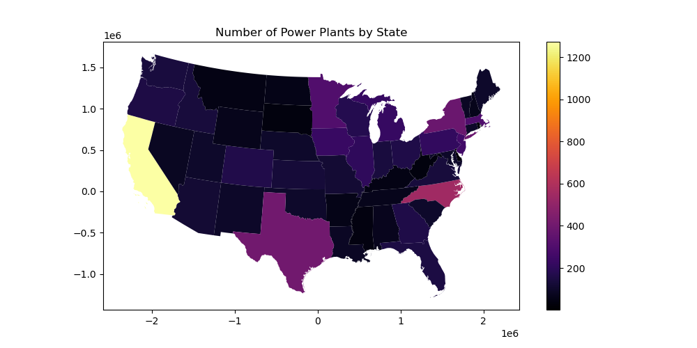
Create a choropleth map to visualize the count of power plants in each state#
https://geopandas.readthedocs.io/en/latest/mapping.html#choropleth-maps
# STUDENT CODE HERE
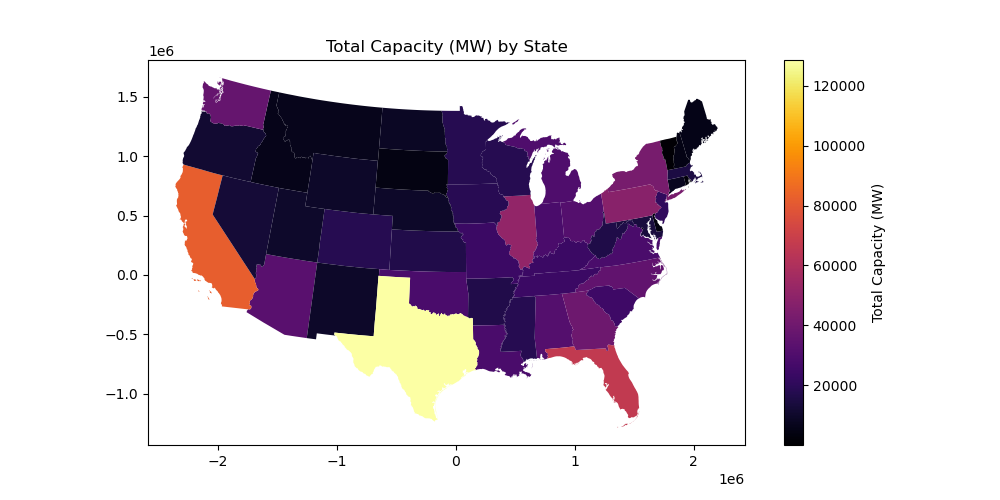
Create a choropleth map to visualize the total power plant capacity in megawatts in each state#
# STUDENT CODE HERE
Part 4: Point density visualization: hexbin plots (2 pts)#
OK, now we have statistics and plots for our existing polygons. But what if we want to compute similar statistics for a regularly spaced grid of cells? For our count, this will give us point density, allowing for better visualization of the spatial distribution.
We could define a set of adjacent rectangular polygons, and repeat our sjoin, groupby, agg sequence above. Or we can use some existing matplotlib functionality, and create a hexbin plot!
Hexagonal cells are preferable over a standard square/rectangular grid for various reasons, especially since projection distortion impacts spatial binning.
Here are some resources on generating hexbins using Python and matplotlib:
https://matplotlib.org/api/_as_gen/matplotlib.pyplot.hexbin.html
http://darribas.org/gds15/content/labs/lab_09.html
Note: an equal-area projection is always good idea for a hexbin plot. Fortunately, we started with our AEA projection, so we’re all set!
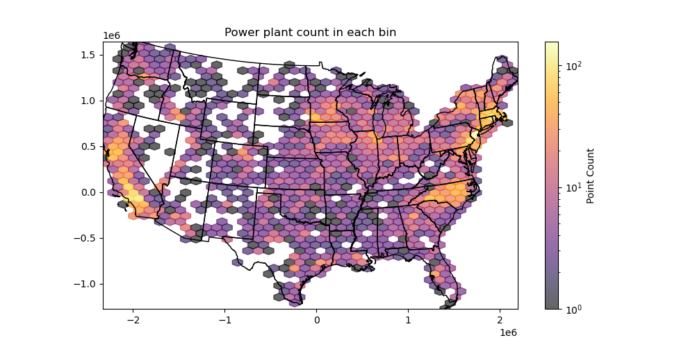
Create a hexbin that shows the number of power plants in each cell#
Play around with the
gridsizeoption to set the number of bins in each dimension (or specify the dimensions of your bins)Use the
mincntoption to avoid plotting cells with 0 countOverlay the state polygons to help visualize
Set your plot
xlimandylimto the power plant point boundsCan use linear color ramp with vmin and vmax options, or try a logarithmic color ramp, since we have a broad range of counts
# STUDENT CODE HERE
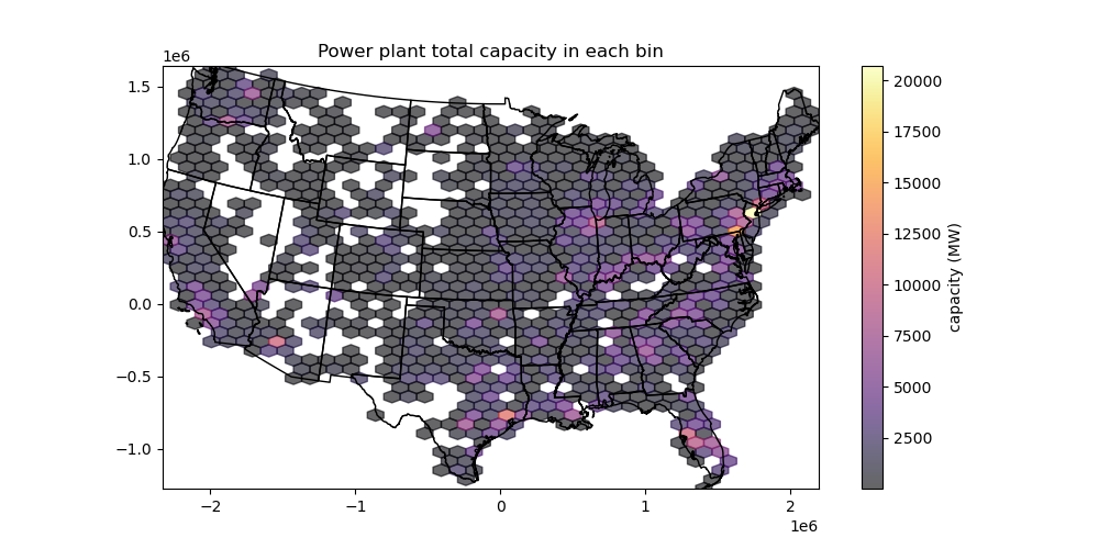
Create a second hexbin plot that shows the total energy generation capacity in each cell#
See documentation for the
Candreduce_C_functionoptions
# STUDENT CODE HERE
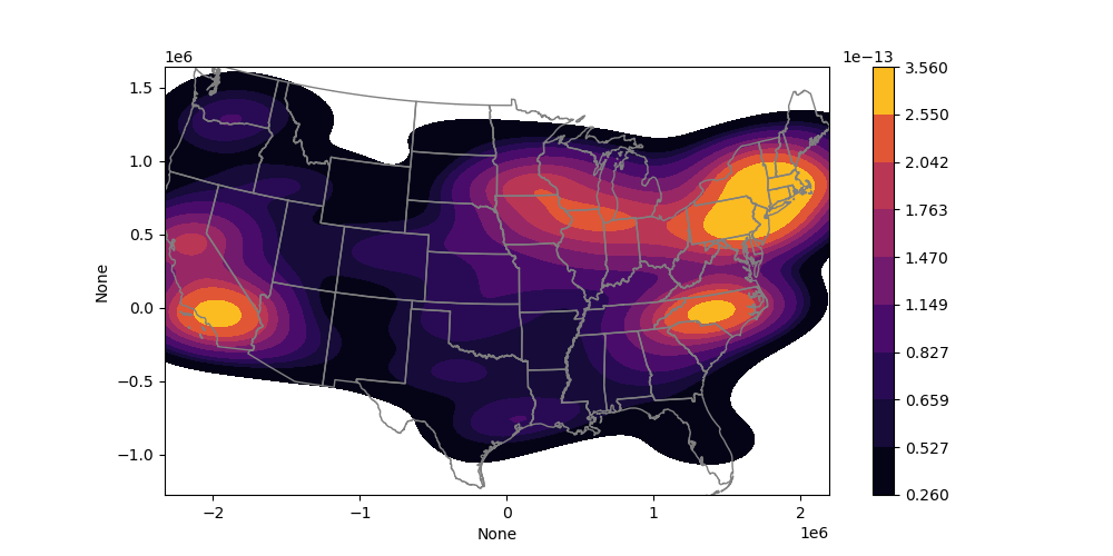
Challenge question (GS required/UG +0.5): Generate a Kernel Density Estimator (KDE) plot using seaborn#
This is another nice approach to estimate the point density on a continuous grid
See motivation here for an explanation: https://en.wikipedia.org/wiki/Multivariate_kernel_density_estimation#Motivation
Seaborn has a nice implementation for 2D data
https://seaborn.pydata.org/generated/seaborn.kdeplot.html#seaborn.kdeplot
https://seaborn.pydata.org/tutorial/distributions.html
# STUDENT CODE HERE
Static plots with tiled basemaps using contextily#
Our state outlines provide some context for our plots, but what if we want a raster map background
Freely available tiled web maps are great: https://en.wikipedia.org/wiki/Tiled_web_map
Can use the convenient
contextilypackage for this: https://github.com/geopandas/contextily
Plot the WA points using our custom projected coordinate system#
Make sure to pass in the appropriate CRS object to
add_basemapFor the particular basemap, try
ctx.providers.Esri.WorldImagery, and then at least one additional differentctx.provider
# STUDENT CODE HERE
Repeat for WA state#
Thought question: Do you note anything about the relationship between power plant locations and rivers in Washington?
# STUDENT CODE HERE
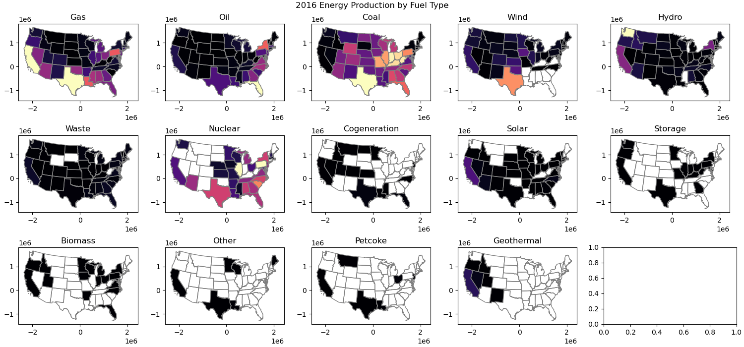
Challenge Question (GS required/UG +0.5): Make a figure with choropleth maps showing total energy generated in 2016 from each different source in each state.#
Use a loop for this
Could use a structure like
for fuel,ax in zip(pplant_gdf_aea_states.fuel1.unique(), axs.flatten()):
Use the
fuel1andgwh_2016columnsSet a common vmin and vmax to enable comparison between maps
Use string formatting to label each plot appropriately
# STUDENT CODE HERE
Part 5: Interactive plots (2 pts)#
See standalone notebook
Please submit this interactive notebook with all plots commented out (completion grade!)
Part 6: Exploring King County Census data (3 pts)#
Below are two functions for getting US Census data and Census tract geometries#
check out the censusdata package: https://github.com/jtleider/censusdata
def get_census_data(tables, state, county, year=2019):
    '''Download census data for a given state and county fips code.'''

    # Download the data
    data = censusdata.download('acs5', year,  # Use 2019 ACS 5-year estimates
                               censusdata.censusgeo([('state', state), ('county', county), ('tract', '*')]),
                               list(tables.keys()))

    # Rename the column
    data.rename(columns=tables, inplace=True)

    # Extract information from the first column
    data['Name'] = data.index.to_series().apply(lambda x: x.name)
    data['SummaryLevel'] = data.index.to_series().apply(lambda x: x.sumlevel())
    data['State'] = data.index.to_series().apply(lambda x: x.geo[0][1])
    data['County'] = data.index.to_series().apply(lambda x: x.geo[1][1])
    data['Tract'] = data.index.to_series().apply(lambda x: x.geo[2][1])
    data.reset_index(drop=True, inplace=True)
    data = data[['Tract','Name']+list(tables.values())].set_index('Tract')

    return data

def get_census_tract_geom(state_fips, county_fips):
    '''Download census tract geometries for a given state and county fips code, storing in /tmp and cleaning up after.'''

    temp_dir = "/tmp/census_tracts"
    zip_path = os.path.join(temp_dir, f'tl_2019_{state_fips}_tract.zip')

    # Ensure temp directory exists
    os.makedirs(temp_dir, exist_ok=True)

    # Download the file
    url = f'https://www2.census.gov/geo/tiger/TIGER2019/TRACT/tl_2019_{state_fips}_tract.zip'
    response = requests.get(url, stream=True)
    if response.status_code != 200:
        raise Exception(f"Failed to download file: {url}")

    # Save ZIP file to temp directory
    with open(zip_path, "wb") as file:
        file.write(response.content)

    # Extract the ZIP file
    with zipfile.ZipFile(zip_path, "r") as zip_ref:
        zip_ref.extractall(temp_dir)

    # Find the shapefile in extracted contents
    for file in os.listdir(temp_dir):
        if file.endswith(".shp"):
            shapefile_path = os.path.join(temp_dir, file)
            break

    # Read the shapefile into a GeoDataFrame
    tracts = gpd.read_file(shapefile_path)

    # Filter by county and set index
    tracts = tracts[tracts['COUNTYFP'] == county_fips]
    tracts = tracts.rename(columns={'TRACTCE': 'Tract'}).set_index('Tract')

    # Cleanup: Remove extracted files and ZIP file
    shutil.rmtree(temp_dir)

    return tracts[['geometry']]
Define our areas of interest#
Both functions will require Federal Information Processing System (FIPS) codes that identify geographic areas
I’ve started you with the correct state and county fips codes, but you can find more here: https://www.census.gov/geographies/reference-files/2017/demo/popest/2017-fips.html
# Define the state and county for Seattle
state_fips = '53'  # FIPS code for Washington
county_fips = '033'  # FIPS code for King County
Define our variables of interest#
I’ve started you with some of the most common variables, feel free to add your own and explore
Check out additional table IDs: https://www.census.gov/programs-surveys/acs/data/data-tables/table-ids-explained.html
Some variables we will have to calculate on our own :)
tables = {
'B19013_001E': 'MedianIncome',
'B01003_001E': 'TotalPopulation',
'B01002_001E': 'MedianAge',
'B17001_002E': 'PopulationBelowPovertyLevel',
'B02001_002E': 'PopulationWhiteAlone',
'B02001_003E': 'PopulationBlackAlone',
'B02001_004E': 'PopulationAmericanIndianAlaskaNativeAlone',
'B02001_005E': 'PopulationAsianAlone',
'B02001_006E': 'PopulationNativeHawaiianPacificIslanderAlone',
'B02001_007E': 'PopulationSomeOtherRaceAlone',
'B02001_008E': 'PopulationTwoOrMoreRaces',
'B03002_003E': 'PopulationNotHispanicWhiteAlone',
'B03003_003E': 'PopulationHispanic',
'B25064_001E': 'MedianGrossRent',
'B25077_001E': 'MedianHomeValue',
'B25035_001E': 'MedianYearStructureBuilt',
'B25001_001E': 'TotalHousingUnits',
'B25004_001E': 'TotalVacantHousingUnits',
'B25003_002E': 'OccupiedHousingUnitsOwnerOccupied',
'B25003_003E': 'OccupiedHousingUnitsRenterOccupied',
'B27001_005E': 'PopulationNoHealthInsuranceCoverage',
}
Pull in the census data#
census_df = get_census_data(tables, state_fips, county_fips)
census_df.head()
| Name | MedianIncome | TotalPopulation | MedianAge | PopulationBelowPovertyLevel | PopulationWhiteAlone | PopulationBlackAlone | PopulationAmericanIndianAlaskaNativeAlone | PopulationAsianAlone | PopulationNativeHawaiianPacificIslanderAlone | ... | PopulationNotHispanicWhiteAlone | PopulationHispanic | MedianGrossRent | MedianHomeValue | MedianYearStructureBuilt | TotalHousingUnits | TotalVacantHousingUnits | OccupiedHousingUnitsOwnerOccupied | OccupiedHousingUnitsRenterOccupied | PopulationNoHealthInsuranceCoverage | |
|---|---|---|---|---|---|---|---|---|---|---|---|---|---|---|---|---|---|---|---|---|---|
| Tract | |||||||||||||||||||||
| 020700 | Census Tract 207, King County, Washington | 82367 | 4064 | 39.4 | 406 | 2555 | 434 | 10 | 671 | 20 | ... | 2109 | 602 | 1617 | 489000 | 1974 | 1581 | 0 | 777 | 804 | 0 |
| 020800 | Census Tract 208, King County, Washington | 116563 | 4279 | 48.9 | 217 | 3618 | 64 | 19 | 423 | 0 | ... | 3420 | 207 | 1328 | 706900 | 1963 | 1787 | 39 | 1348 | 400 | 0 |
| 020900 | Census Tract 209, King County, Washington | 103690 | 3420 | 43.6 | 271 | 2378 | 342 | 5 | 439 | 0 | ... | 2366 | 118 | 1243 | 590100 | 1973 | 1511 | 181 | 955 | 375 | 0 |
| 021000 | Census Tract 210, King County, Washington | 98083 | 6024 | 41.4 | 369 | 3587 | 455 | 87 | 1254 | 67 | ... | 3339 | 564 | 1752 | 477600 | 1962 | 2363 | 193 | 1618 | 552 | 0 |
| 022001 | Census Tract 220.01, King County, Washington | 102143 | 5729 | 43.8 | 236 | 4107 | 35 | 14 | 473 | 56 | ... | 3963 | 687 | 1407 | 636600 | 1989 | 2473 | 93 | 1397 | 983 | 0 |
5 rows × 22 columns
Let’s calculate our own variables#
Create new columns in your census_data_gdf for…
RatioMedianGrossRentToIncome
PercentRented
PercentOwned
PopulationNonWhite (TotalPopulation - PopulationNotHispanicWhiteAlone)
# STUDENT CODE HERE
Now let’s use this convert_to_percentages() function to convert our raw population numbers to percentages#
def convert_to_percentages(df, total_population_column='TotalPopulation'):
    '''Converts population counts to percentages'''
    for column in df.columns:
        if column.startswith('Population'):
            new_column_name = 'Percent' + column
            df[new_column_name] = (df[column] / df[total_population_column]) * 100
            df.drop(column, axis=1, inplace=True)
    return df
census_df = convert_to_percentages(census_df)
census_df.head()
| Name | MedianIncome | TotalPopulation | MedianAge | MedianGrossRent | MedianHomeValue | MedianYearStructureBuilt | TotalHousingUnits | TotalVacantHousingUnits | OccupiedHousingUnitsOwnerOccupied | ... | PercentPopulationBlackAlone | PercentPopulationAmericanIndianAlaskaNativeAlone | PercentPopulationAsianAlone | PercentPopulationNativeHawaiianPacificIslanderAlone | PercentPopulationSomeOtherRaceAlone | PercentPopulationTwoOrMoreRaces | PercentPopulationNotHispanicWhiteAlone | PercentPopulationHispanic | PercentPopulationNoHealthInsuranceCoverage | PercentPopulationNonWhite | |
|---|---|---|---|---|---|---|---|---|---|---|---|---|---|---|---|---|---|---|---|---|---|
| Tract | |||||||||||||||||||||
| 020700 | Census Tract 207, King County, Washington | 82367 | 4064 | 39.4 | 1617 | 489000 | 1974 | 1581 | 0 | 777 | ... | 10.679134 | 0.246063 | 16.510827 | 0.492126 | 3.764764 | 5.437992 | 51.894685 | 14.812992 | 0.0 | 48.105315 |
| 020800 | Census Tract 208, King County, Washington | 116563 | 4279 | 48.9 | 1328 | 706900 | 1963 | 1787 | 39 | 1348 | ... | 1.495677 | 0.444029 | 9.885487 | 0.000000 | 0.210330 | 3.412012 | 79.925216 | 4.837579 | 0.0 | 20.074784 |
| 020900 | Census Tract 209, King County, Washington | 103690 | 3420 | 43.6 | 1243 | 590100 | 1973 | 1511 | 181 | 955 | ... | 10.000000 | 0.146199 | 12.836257 | 0.000000 | 2.573099 | 4.912281 | 69.181287 | 3.450292 | 0.0 | 30.818713 |
| 021000 | Census Tract 210, King County, Washington | 98083 | 6024 | 41.4 | 1752 | 477600 | 1962 | 2363 | 193 | 1618 | ... | 7.553121 | 1.444223 | 20.816733 | 1.112218 | 1.377822 | 8.150730 | 55.428287 | 9.362550 | 0.0 | 44.571713 |
| 022001 | Census Tract 220.01, King County, Washington | 102143 | 5729 | 43.8 | 1407 | 636600 | 1989 | 2473 | 93 | 1397 | ... | 0.610927 | 0.244371 | 8.256240 | 0.977483 | 9.128993 | 9.094083 | 69.174376 | 11.991622 | 0.0 | 30.825624 |
5 rows × 26 columns
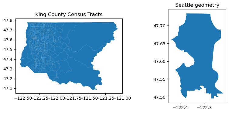
Let’s add geometries for the census tracts and Seattle#
Pull in the census geometries using the provided get_census_tract_geom() using the same FIPS codes
Geojson of Seattle available here: https://github.com/seattleflu/seattle-geojson
tract_geom_gdf = get_census_tract_geom(state_fips, county_fips)
seattle_gdf = gpd.read_file('https://raw.githubusercontent.com/seattleflu/seattle-geojson/master/seattle_geojsons/2016_seattle_city.geojson', engine='pyogrio')
f,ax=plt.subplots(1,2,figsize=(10,4))

tract_geom_gdf.plot(ax=ax[0])
seattle_gdf.plot(ax=ax[1])

ax[0].set_title('King County Census Tracts')
ax[1].set_title('Seattle geometry')
Text(0.5, 1.0, 'Seattle geometry')
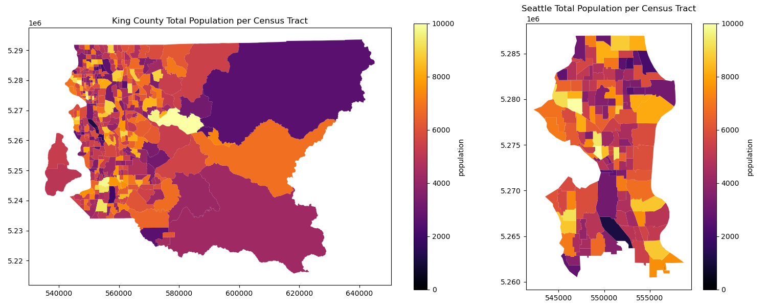
Combine the census data and census tract geometry and plot#
You can try .join() to create a combined dataframe
what should you put for the “how” argument?
If it is not already, convert the dataframe into a geodataframe
census_kc_gdfWhat crs is the new geodataframe in? reproject it to EPSG:32610!
Filter your new census_data_gdf by ‘TotalPopulation’ > 0 to get rid of empty tracts
Make sure your Seattle geodataframe is also in EPSG:32610, then use the .clip() operation to create
census_sea_gdfCreate a figure with two total population choropleth plots, one for King County, and one for Seattle
# STUDENT CODE HERE
# STUDENT CODE HERE
# STUDENT CODE HERE
# STUDENT CODE HERE
# STUDENT CODE HERE
Written response: Explore the map#
Use geopandas .explore() on
census_kc_gdfto explore the mapPass in a variable of interest to column
Be mindful of your vmin and vmax settings!
At submission time, please comment out this cell to reduce notebook size at turn in :)
Tell us something you saw!
# STUDENT CODE HERE
STUDENT WRITTEN RESPONSE HERE
Get a rough idea of variable correlation#
Use the pandas built-in .corr() functionality and store the correlation matrix in census_corr
Pass in numeric_only=True to avoid errors
Pass in census_corr to sns.heatmap() to visualize the correlations
# STUDENT CODE HERE
# STUDENT CODE HERE
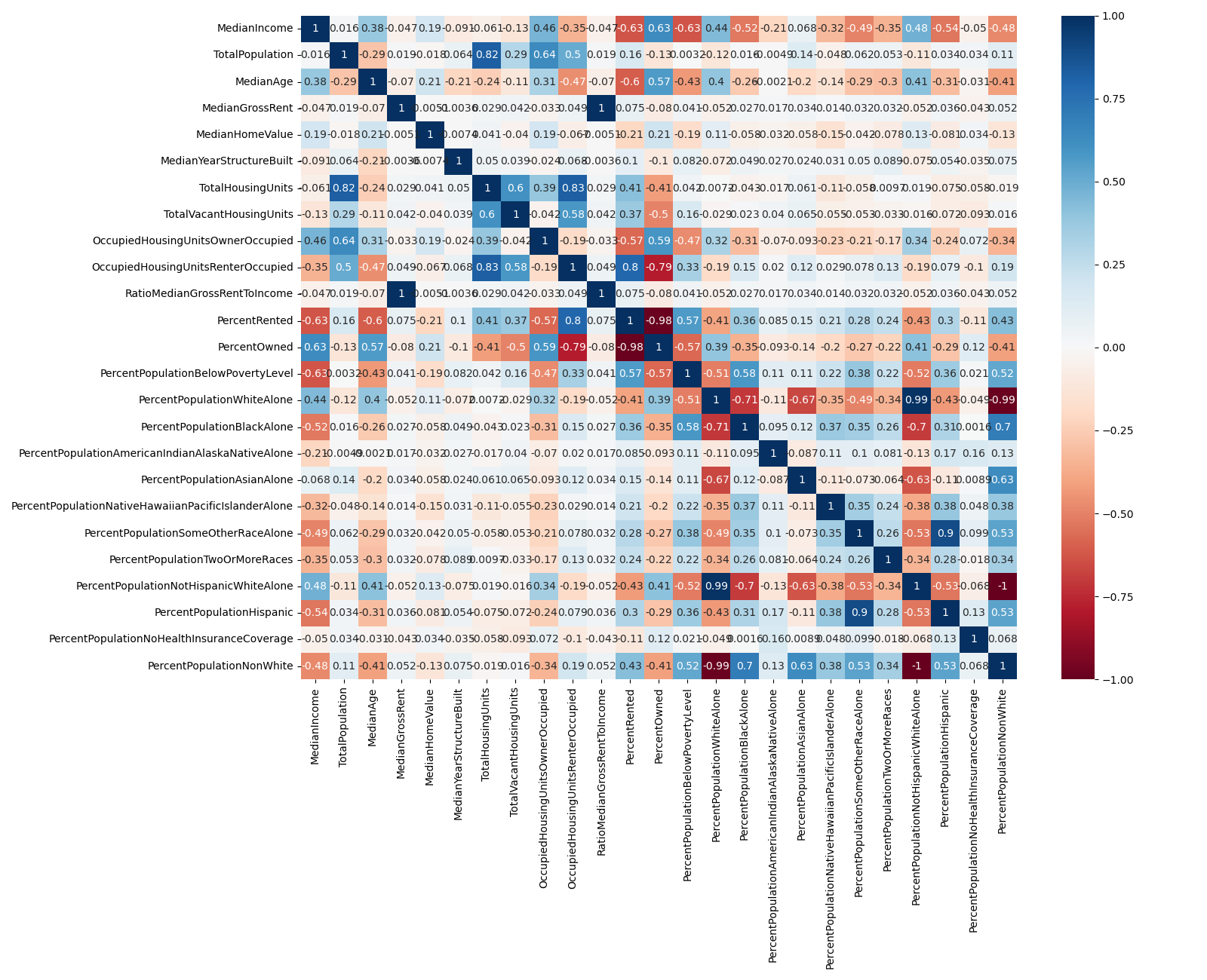
Written response: Try the variable correlation above for both census_kc_gdf and also census_sea_gdf What do you see?#
STUDENT WRITTEN RESPONSE HERE
Explore one of these relationships with a scatterplot#
Try your own, don’t copy the example!
Besides plotting some variable on x and y, try setting the color/size of your points to another variable as well
# STUDENT CODE HERE
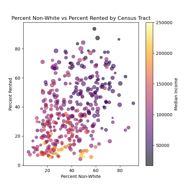
Written response: Describe an insight from the exploration of your plot!#
STUDENT WRITTEN RESPONSE HERE
Part 7: Distribution of toxic releases in King County (4 pts)#
Let’s explore how toxic releases are distributed across our census tracts. For this, let’s use the Toxic Release Inventory (TRI)
From the TRI website: “TRI tracks the management of certain toxic chemicals that may pose a threat to human health and the environment. U.S. facilities in different industry sectors must report annually how much of each chemical is released to the environment and/or managed through recycling, energy recovery and treatment. (A “release” of a chemical means that it is emitted to the air or water, or placed in some type of land disposal.)”
TRI has all sorts of information for the US, but we are going to be focused on releases in King County
Read more about the TRI here: https://www.epa.gov/toxics-release-inventory-tri-program/what-toxics-release-inventory
Let’s bring in the Toxic release data as a geodataframe in the correct crs#
For the sake of time, we’ve done done this for you and saved a geojson to the data folder.
The code to do this is preserved below
# def get_tri_data(year=2019):
#     '''Get the Toxic Release Inventory data for a given year'''
#     url = f'https://data.epa.gov/efservice/downloads/tri/mv_tri_basic_download/{year}_US/csv'
#     columns_of_interest = ['2. TRIFD','4. FACILITY NAME','8. ST','23. INDUSTRY SECTOR','37. CHEMICAL','65. ON-SITE RELEASE TOTAL', '12. LATITUDE','13. LONGITUDE']
#     tri_data = pd.read_csv(url,usecols=columns_of_interest)
#     tri_data = pd.read_csv(url)
#     tri_data = tri_data[columns_of_interest]
#     tri_data.columns = tri_data.columns.str.replace('^[0-9. ]*', '', regex=True)
#     return tri_data
# tri_df = pd.DataFrame()

# for year in range(1987,2022):
#     tri_df = pd.concat([tri_df,get_tri_data(year)])
# tri_df
# tri_wa_df = tri_df[tri_df['ST'] == 'WA']
# tri_wa_df = tri_wa_df.reset_index(drop=True)
# tri_wa_gdf = gpd.GeoDataFrame(tri_wa_df, geometry=gpd.points_from_xy(tri_wa_df.LONGITUDE, tri_wa_df.LATITUDE)).set_crs('EPSG:4326').to_crs('EPSG:32610')
# tri_kc_gdf = gpd.sjoin(tri_wa_gdf, tract_geom_gdf.to_crs(32610), predicate="intersects")
# tri_kc_gdf = tri_kc_gdf.reset_index(drop=True)
# tri_kc_gdf = tri_kc_gdf.drop(columns='Tract')
# tri_kc_gdf.to_file("data/tri_kc.geojson", driver="GeoJSON")
# read in data
tri_kc_gdf = gpd.read_file('data/tri_kc.geojson')
Clip locations to the convex hull of our census data#
Remember to do the unary_union before using convex hull!
Hint: use intersects :)
# STUDENT CODE HERE
Sort the geodataframe by ON-SITE RELEASE TOTAL#
# STUDENT CODE HERE
| TRIFD | FACILITY NAME | ST | INDUSTRY SECTOR | CHEMICAL | ON-SITE RELEASE TOTAL | LATITUDE | LONGITUDE | geometry | |
|---|---|---|---|---|---|---|---|---|---|
| 662 | 98106STTLS2414S | SEATTLE STEEL INC | WA | Primary Metals | Aluminum oxide (fibrous forms) | 2138500.0 | 47.569331 | -122.367332 | POINT (547585.548 5268628.876) |
| 683 | 98108THBNG7500E | BOEING COMMERCIAL AIRPLANE GROUP NORTH BOEING ... | WA | Transportation Equipment | Trichloroethylene | 682000.0 | 47.531169 | -122.310812 | POINT (551874.276 5264423.885) |
| 774 | 98108RHNPL9229E | RHONE-POULENC INC | WA | Chemicals | Toluene | 636166.0 | 47.520258 | -122.303946 | POINT (552401.934 5263215.89) |
| 565 | 98108RHNPL9229E | RHONE-POULENC INC | WA | Chemicals | Toluene | 570000.0 | 47.520258 | -122.303946 | POINT (552401.934 5263215.89) |
| 1853 | 98002BNGCM70015 | BOEING COMMERCIAL AIRPLANES - AUBURN | WA | Transportation Equipment | 1,1,1-Trichloroethane | 570000.0 | 47.283625 | -122.242770 | POINT (557263.362 5236961.139) |
| ... | ... | ... | ... | ... | ... | ... | ... | ... | ... |
| 5598 | 98032BRLNG20245 | BURLINGTON ENVIRONMENTAL LLC | WA | Hazardous Waste | Nitrate compounds (water dissociable; reportab... | 0.0 | 47.418259 | -122.238184 | POINT (557463.831 5251926.719) |
| 7190 | 98032VNWTR8201S | UNIVAR SOLUTIONS KENT | WA | Chemical Wholesalers | Toluene | 0.0 | 47.411106 | -122.230700 | POINT (558036.206 5251137.334) |
| 7191 | 98032XTCMT5411S | EXOTIC METALS FORMING CO | WA | Transportation Equipment | Nickel compounds | 0.0 | 47.399148 | -122.264995 | POINT (555461.544 5249783.393) |
| 2320 | 98032MRCNN1220N | REXAM BEVERAGE CAN CO RE: KENT WA FACILITY | WA | Fabricated Metals | Nitric acid | 0.0 | 47.404217 | -122.238960 | POINT (557420.559 5250365.608) |
| 3636 | 98108TMPRS701SO | TRIM SYSTEMS | WA | Plastics and Rubber | Ethylene glycol | 0.0 | 47.538461 | -122.325001 | POINT (550799.249 5265224.911) |
9147 rows × 9 columns
Written response: What do you notice? What are the lowest values, and why do you think those are the lowest values?#
STUDENT WRITTEN RESPONSE HERE
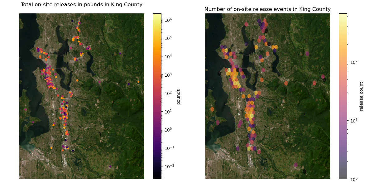
Make a figure with two plots. On the left, the ON-SITE RELEASE TOTAL as points, and on the right, a hexbin plot of release_count.#
Make the colorscale logarithmic
# STUDENT CODE HERE
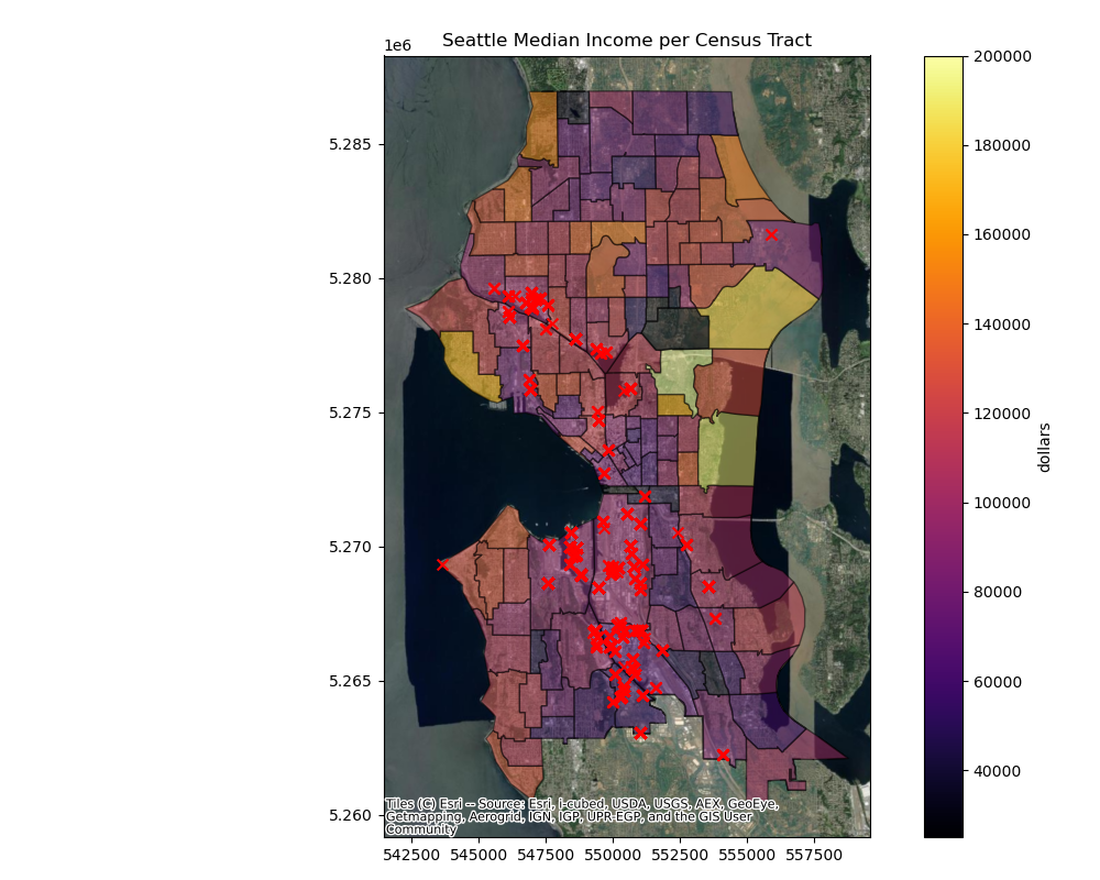
Plot the release sites on top of the median income census data#
Now focus on Seattle: create
tri_sea_gdfby clippingtri_kc_gdfPlot
tri_sea_gdfon top of ‘MedianIncome’ fromcensus_sea_gdf
# STUDENT CODE HERE
# STUDENT CODE HERE
Written response: What do you notice about the distribution of toxic releases as it relates to median income?#
STUDENT WRITTEN RESPONSE HERE
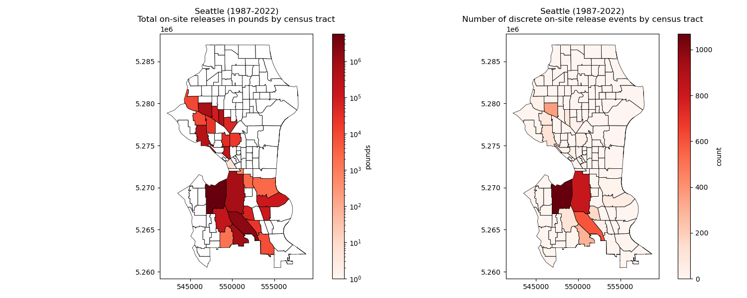
Do a spatial join to get the census tract for each facility in Seattle#
First buffer each facility by 100m
Then join the facilities with the census tracts
Find the total releases in pounds per tract (groupby tract, then sum)
Find the total number of discrete release events per tract (groupby tract, then count)
tri_sea_gdf.loc[:,'geometry'] = tri_sea_gdf.buffer(100)
# STUDENT CODE HERE
census_sea_gdf['TRI_RELEASE_SUM'] = tri_sea_join_census_gdf.groupby('Tract')['ON-SITE RELEASE TOTAL'].sum().sort_index()
census_sea_gdf['TRI_RELEASE_SUM'] = census_sea_gdf['TRI_RELEASE_SUM'].fillna(0)
# STUDENT CODE HERE
Create choropleth maps of Seattle: one for total on-site release (pounds), and one for number of discrete on-site release events#
# STUDENT CODE HERE
Written response: Take a moment to reflect. What do you see?#
STUDENT WRITTEN RESPONSE HERE
Submit your work#
Save this notebook with all code and output (Make sure when you save the notebook, all cells show their outputs).
Use the terminal to stage, commit, and push your notebook to your GitHub repository. It should look something like this…
git add 01_lab.ipynb
git commit -m “Completed Lab 01 exercises”
git push
Verify that your notebook appears in your GitHub repository. Double check to make sure all the ouputs are visible!