Lab 04 assignment notebook 2 (20 pts)#
Notebook 2 of 2
UW Geospatial Data Analysis
CEE467/CEWA567
David Shean, Eric Gagliano, Quinn Brencher
Part 0: Setup from Notebook #1#
import geopandas as gpd
import rasterio as rio
import rioxarray as rxr
import matplotlib.pyplot as plt
from matplotlib_scalebar.scalebar import ScaleBar
from pathlib import Path
import os
import numpy as np
import xarray as xr
#May want to use interactive plotting for zoom/pan and live coordinate display
#%matplotlib widget
%matplotlib inline
imgdir = f'{Path.home()}/gda_demo_data/LS8_data'
!ls -lh $imgdir
total 1.3G
-rw-r--r-- 1 eric eric 1.2M Jan 26 11:31 LC08_L2SP_046027_20180818_02_T1_rendered_preview.png
-rw-r--r-- 1 eric eric  81M Jan 26 11:27 LC08_L2SP_046027_20180818_20200831_02_T1_SR_B1.TIF
-rw-r--r-- 1 eric eric  81M Jan 26 11:28 LC08_L2SP_046027_20180818_20200831_02_T1_SR_B2.TIF
-rw-r--r-- 1 eric eric  82M Jan 26 11:28 LC08_L2SP_046027_20180818_20200831_02_T1_SR_B3.TIF
-rw-r--r-- 1 eric eric  83M Jan 26 11:29 LC08_L2SP_046027_20180818_20200831_02_T1_SR_B4.TIF
-rw-r--r-- 1 eric eric  92M Jan 26 11:29 LC08_L2SP_046027_20180818_20200831_02_T1_SR_B5.TIF
-rw-r--r-- 1 eric eric  90M Jan 26 11:30 LC08_L2SP_046027_20180818_20200831_02_T1_SR_B6.TIF
-rw-r--r-- 1 eric eric  84M Jan 26 11:31 LC08_L2SP_046027_20180818_20200831_02_T1_ST_B10.TIF
-rw-r--r-- 1 eric eric 115M Jan 27 19:39 LC08_L2SP_046027_20180818_20200831_02_T1_ST_B10_4326.TIF
-rw-r--r-- 1 eric eric 1.5M Jan 26 11:27 LC08_L2SP_046027_20181224_02_T1_rendered_preview.png
-rw-r--r-- 1 eric eric  91M Jan 26 11:23 LC08_L2SP_046027_20181224_20200829_02_T1_SR_B1.TIF
-rw-r--r-- 1 eric eric  91M Jan 26 11:24 LC08_L2SP_046027_20181224_20200829_02_T1_SR_B2.TIF
-rw-r--r-- 1 eric eric  92M Jan 26 11:24 LC08_L2SP_046027_20181224_20200829_02_T1_SR_B3.TIF
-rw-r--r-- 1 eric eric  91M Jan 26 11:25 LC08_L2SP_046027_20181224_20200829_02_T1_SR_B4.TIF
-rw-r--r-- 1 eric eric  96M Jan 26 11:26 LC08_L2SP_046027_20181224_20200829_02_T1_SR_B5.TIF
-rw-r--r-- 1 eric eric  90M Jan 26 11:26 LC08_L2SP_046027_20181224_20200829_02_T1_SR_B6.TIF
-rw-r--r-- 1 eric eric  77M Jan 26 11:27 LC08_L2SP_046027_20181224_20200829_02_T1_ST_B10.TIF
#Pre-identified cloud-free Image IDs used for the lab
august_id = 'LC08_L2SP_046027_20180818_20200831_02_T1' # August 2018
december_id = 'LC08_L2SP_046027_20181224_20200829_02_T1' # # December 2018
# B10 is the thermal infrared /surface temperture band
tir_august_fn = os.path.join(imgdir, august_id+'_ST_B10.TIF')
tir_december_fn = os.path.join(imgdir, december_id+'_ST_B10.TIF')

swir_august_fn = os.path.join(imgdir, august_id+'_SR_B6.TIF')
swir_december_fn = os.path.join(imgdir, december_id+'_SR_B6.TIF')

nir_august_fn = os.path.join(imgdir, august_id+'_SR_B5.TIF')
nir_december_fn = os.path.join(imgdir, december_id+'_SR_B5.TIF')

red_august_fn = os.path.join(imgdir, august_id+'_SR_B4.TIF')
red_december_fn = os.path.join(imgdir, december_id+'_SR_B4.TIF')

green_august_fn = os.path.join(imgdir, august_id+'_SR_B3.TIF')
green_december_fn = os.path.join(imgdir, december_id+'_SR_B3.TIF')

blue_august_fn = os.path.join(imgdir, august_id+'_SR_B2.TIF')
blue_december_fn = os.path.join(imgdir, december_id+'_SR_B2.TIF')
We’ve had practice opening Landsat-8 data using rioxarray, squeezing, selecting a window, masking, and scaling to a geophysical variable! Since we’re going to repeat this process many more times for the remainder of this lab, let’s build a quick function that accepts a filename amd returns a raster of the given geophysical variable over Mt. Rainier as a masked Xarray DataArray#
#Scale and offset values for L2 Landsat products
#Surface Reflectance 0.0000275 + -0.2
sr_scale = 0.0000275
sr_offset = -0.2

st_scale = 0.00341802
st_offset = 149.0

rainier_x_slice = slice(581685.0, 612405.0)
rainier_y_slice = slice(5205615.0, 5174895.0)

def rxr_read_crop_mask_scale_ls8(fn):
    """Pass in a filename, read the raster file with rioxarray, mask nodata values, and scale to either surface reflectance or surface temperature"""
    da = rxr.open_rasterio(fn,masked=True).squeeze().sel(x=rainier_x_slice, y=rainier_y_slice)

    if fn.endswith('ST_B10.TIF'):
        da = da * st_scale + st_offset
        da = da - 273.15
    else:
        da = da * sr_scale + sr_offset

    return da
Part 6: Composite images (3 pts)#
First, please take a look at this quick explainer on composite imagery.
The many bands of Landsat-8 allow for diverse composite images with different use cases.
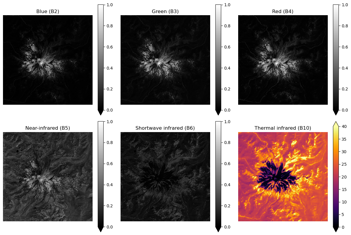
Let’s take a look at all of the bands we downloaded for the August 2018 acqusition#
all_august_bands = [blue_august_fn, green_august_fn, red_august_fn, nir_august_fn, swir_august_fn, tir_august_fn]
f,axs=plt.subplots(2,3,figsize=(12,8))

band_names = ['Blue', 'Green', 'Red', 'Near-infrared', 'Shortwave infrared', 'Thermal infrared']
for band,ax in zip(all_august_bands, axs.flat):

    da = rxr_read_crop_mask_scale_ls8(band)

    if 'ST' in band:
        da.plot.imshow(ax=ax,cmap='inferno',vmin=0,vmax=40)
    else:
        da.plot.imshow(ax=ax,cmap='gray',vmin=0,vmax=1)


    ax.set_title(f"{band_names.pop(0)} ({band.split('_')[-1].split('.')[0]})")

    ax.axis('off')

    ax.set_aspect('equal')

f.tight_layout()
Let’s plot some composite images!#
First, figure out what bands you’ll need and read them in using the helper function we just defined
rxr_read_crop_mask_scale_ls8(fn)For example
red_august_da = rxr_read_crop_mask_scale_ls8(red_august_fn)
Use xarray’s concat function to merge the xarray DataArrays along a new band dimension
Check out the rioxarray tutorial for a refresher on this
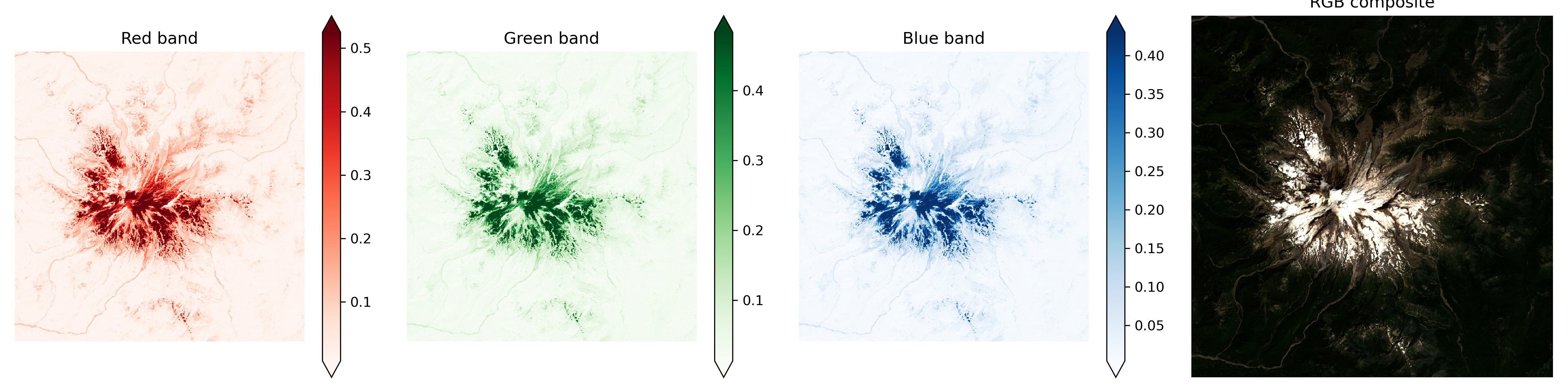
Create a figure with 4 plots: red, green, blue, and the “true” / “natural” RGB composite image#
Try using colormaps that correspond to the band (e.g. ‘Reds’ for the red band)
Set
vmin=0andvmax=1for the single band plots
red_august_da = rxr_read_crop_mask_scale_ls8(red_august_fn)
green_august_da = rxr_read_crop_mask_scale_ls8(green_august_fn)
blue_august_da = rxr_read_crop_mask_scale_ls8(blue_august_fn)
# STUDENT CODE HERE
<xarray.DataArray (band: 3, y: 1024, x: 1024)> Size: 13MB
array([[[0.020495  , 0.021705  , 0.0201925 , ..., 0.01466499,
         0.01210749, 0.00966001],
        [0.0198625 , 0.01933999, 0.01744249, ..., 0.0189275 ,
         0.0096875 , 0.00933   ],
        [0.01681   , 0.01593   , 0.0150225 , ..., 0.01727749,
         0.0115025 , 0.01142   ],
        ...,
        [0.012135  , 0.01031999, 0.0114475 , ..., 0.01263   ,
         0.012575  , 0.01309749],
        [0.011585  , 0.01199751, 0.01252   , ..., 0.0112    ,
         0.01293249, 0.01265749],
        [0.012245  , 0.01232749, 0.0112275 , ..., 0.01504999,
         0.0146925 , 0.0137575 ]],

       [[0.037435  , 0.03922249, 0.0376275 , ..., 0.02602249,
         0.02329999, 0.0221725 ],
        [0.03515249, 0.03427249, 0.0319075 , ..., 0.02731501,
         0.0232725 , 0.024675  ],
        [0.031385  , 0.0281675 , 0.02769999, ..., 0.0280575 ,
         0.0268475 , 0.02791999],
...
        [0.02539   , 0.022695  , 0.0248675 , ..., 0.0283875 ,
         0.0282225 , 0.02959751],
        [0.0244    , 0.02539   , 0.02802999, ..., 0.02627   ,
         0.02858   , 0.02775499],
        [0.02412499, 0.02607749, 0.02462   , ..., 0.030285  ,
         0.03058749, 0.0299    ]],

       [[0.01851501, 0.0185975 , 0.016425  , ..., 0.01285   ,
         0.01131   , 0.01031999],
        [0.0182125 , 0.0160675 , 0.01477499, ..., 0.01628751,
         0.008395  , 0.0095225 ],
        [0.015985  , 0.01351   , 0.01254749, ..., 0.01532499,
         0.00971501, 0.0107325 ],
        ...,
        [0.00801   , 0.00713   , 0.007515  , ..., 0.00922   ,
         0.0092475 , 0.009385  ],
        [0.00746   , 0.00831249, 0.008505  , ..., 0.008725  ,
         0.009385  , 0.0095775 ],
        [0.00842249, 0.00834   , 0.007625  , ..., 0.01064999,
         0.01070499, 0.01070499]]], dtype=float32)
Coordinates:
  * band         (band) int64 24B 1 1 1
  * x            (x) float64 8kB 5.817e+05 5.817e+05 ... 6.124e+05 6.124e+05
  * y            (y) float64 8kB 5.206e+06 5.206e+06 ... 5.175e+06 5.175e+06
spatial_ref int64 8B 0# STUDENT CODE HERE
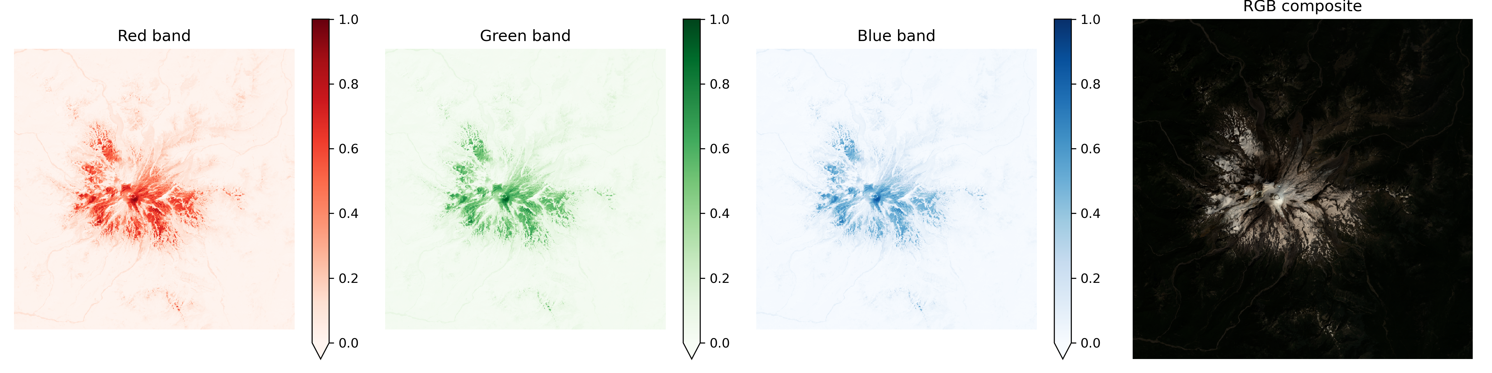
These plots are pretty faint#
Even though the surface reflectance values go from 0 to 1, most of the values are close to 0. Check out the following histograms…
f,axs = plt.subplots(1,3,figsize=(12,3),sharex=True)

red_august_da.plot.hist(ax=axs[0],bins=1000,color='r',alpha=0.5);
green_august_da.plot.hist(ax=axs[1],bins=1000,color='g',alpha=0.5);
blue_august_da.plot.hist(ax=axs[2],bins=1000,color='b',alpha=0.5);

axs[0].set_title('Red band')
axs[1].set_title('Green band')
axs[2].set_title('Blue band')

f.tight_layout()
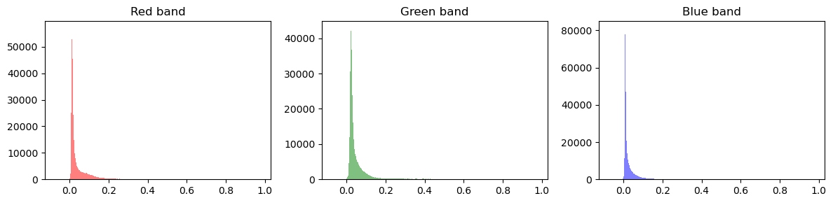
We can address this a couple of ways: we can either change the actual array values, or change how we plot!#
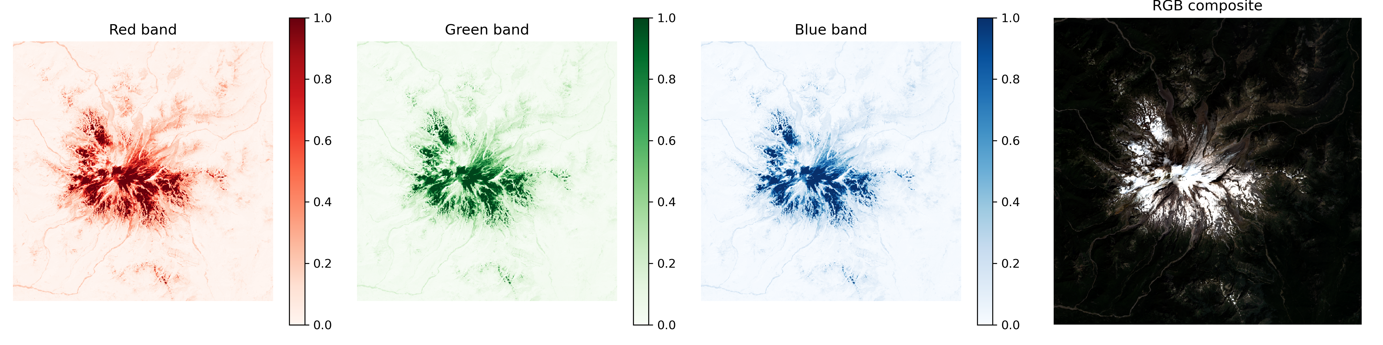
Recreate the figure of the 3 seperate bands and the RGB composite. This time, use the provided function to create a normalized version of each DataArray, mapping the 2nd percentile of values to 0 and the 98th percentile to 1. For the RGB composite, you’ll need to use xr.concat on the newly normalized rasters. Keep vmin=0 and vmax=1#
def percentile_stretch(da, pmin=2, pmax=98):

    min_val = da.quantile(pmin/100)
    max_val = da.quantile(pmax/100)

    stretched = da.clip(min_val,max_val)
    stretched = (stretched - min_val) / (max_val - min_val)

    return stretched
# STUDENT CODE HERE
# STUDENT CODE HERE
red_august_norm_da = None
green_august_norm_da = None
blue_august_norm_da = None
rgb_august_norm_da = None
Now we’ll try it the other way. Recreate the figure of the 3 seperate bands and the RGB composite. This time, for each band, adjust each vmin and vmax such that they represent the 2nd and 98th percentile of the band values. Also, in the rgb image plot call, set robust=True#
Don’t use the normalized DataArrays we just made!
Read about the robust option here
red_percentile_2 = red_august_da.quantile(0.02)
red_percentile_98 = red_august_da.quantile(0.98)

green_percentile_2 = green_august_da.quantile(0.02)
green_percentile_98 = green_august_da.quantile(0.98)

blue_percentile_2 = blue_august_da.quantile(0.02)
blue_percentile_98 = blue_august_da.quantile(0.98)
# STUDENT CODE HERE
Written response: What makes these two approaches to contrast enhancement different? Why might we prefer one over the other?#
STUDENT WRITTEN RESPONSE HERE
Let’s get back to composite images#
Make a similar figure for color-infrared as described in the explainer above. Use robust=True on all plots in the figure#
# STUDENT CODE HERE
# STUDENT CODE HERE
<xarray.DataArray (band: 3, y: 1024, x: 1024)> Size: 13MB
array([[[0.46368504, 0.4773525 , 0.44704753, ..., 0.11834   ,
         0.08800749, 0.09017999],
        [0.4457    , 0.4263125 , 0.3925975 , ..., 0.06653   ,
         0.12034748, 0.157115  ],
        [0.38674003, 0.36611503, 0.3560775 , ..., 0.08327751,
         0.1772175 , 0.19388251],
        ...,
        [0.235215  , 0.21401249, 0.22520499, ..., 0.229385  ,
         0.2224    , 0.2434925 ],
        [0.22704749, 0.2374975 , 0.25086248, ..., 0.2078525 ,
         0.2253425 , 0.229825  ],
        [0.23920251, 0.23975249, 0.22803749, ..., 0.2269925 ,
         0.24143   , 0.2401375 ]],

       [[0.020495  , 0.021705  , 0.0201925 , ..., 0.01466499,
         0.01210749, 0.00966001],
        [0.0198625 , 0.01933999, 0.01744249, ..., 0.0189275 ,
         0.0096875 , 0.00933   ],
        [0.01681   , 0.01593   , 0.0150225 , ..., 0.01727749,
         0.0115025 , 0.01142   ],
...
        [0.012135  , 0.01031999, 0.0114475 , ..., 0.01263   ,
         0.012575  , 0.01309749],
        [0.011585  , 0.01199751, 0.01252   , ..., 0.0112    ,
         0.01293249, 0.01265749],
        [0.012245  , 0.01232749, 0.0112275 , ..., 0.01504999,
         0.0146925 , 0.0137575 ]],

       [[0.037435  , 0.03922249, 0.0376275 , ..., 0.02602249,
         0.02329999, 0.0221725 ],
        [0.03515249, 0.03427249, 0.0319075 , ..., 0.02731501,
         0.0232725 , 0.024675  ],
        [0.031385  , 0.0281675 , 0.02769999, ..., 0.0280575 ,
         0.0268475 , 0.02791999],
        ...,
        [0.02539   , 0.022695  , 0.0248675 , ..., 0.0283875 ,
         0.0282225 , 0.02959751],
        [0.0244    , 0.02539   , 0.02802999, ..., 0.02627   ,
         0.02858   , 0.02775499],
        [0.02412499, 0.02607749, 0.02462   , ..., 0.030285  ,
         0.03058749, 0.0299    ]]], dtype=float32)
Coordinates:
  * band         (band) int64 24B 1 1 1
  * x            (x) float64 8kB 5.817e+05 5.817e+05 ... 6.124e+05 6.124e+05
  * y            (y) float64 8kB 5.206e+06 5.206e+06 ... 5.175e+06 5.175e+06
spatial_ref int64 8B 0# STUDENT CODE HERE
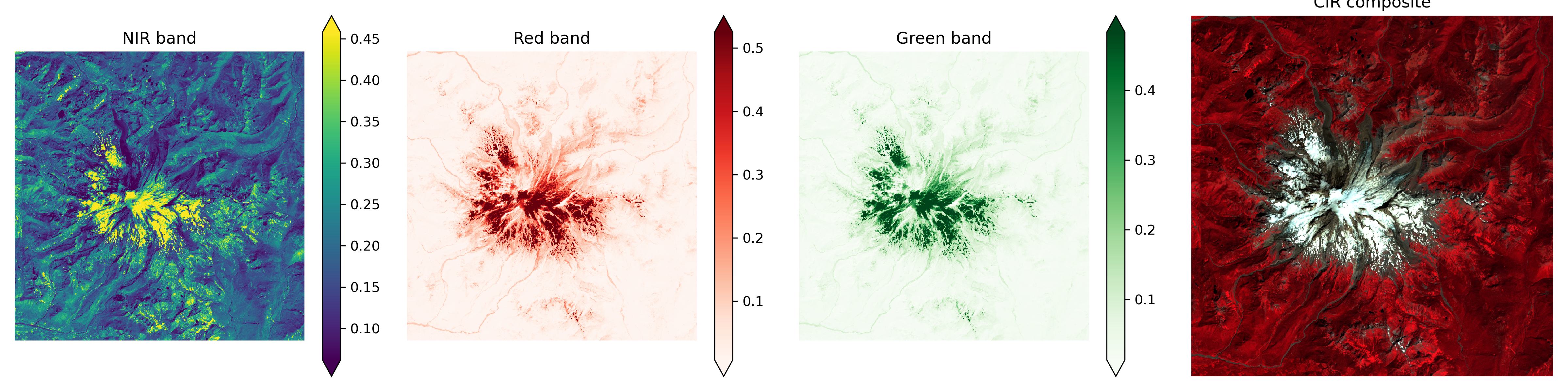
Written response: How might this CIR composite plot be useful?#
STUDENT WRITTEN RESPONSE HERE
Part 7: Raster band math and index ratios (3 pts)#
Let’s use some common band ratios to classify vegetation, snow, and water
Calculate NDVI (normalized difference vegetation index), clip values to [-1,1], and plot with robust=True#
Hint: Use the built-in DataArray method .clip for this!
# STUDENT CODE HERE
# STUDENT CODE HERE
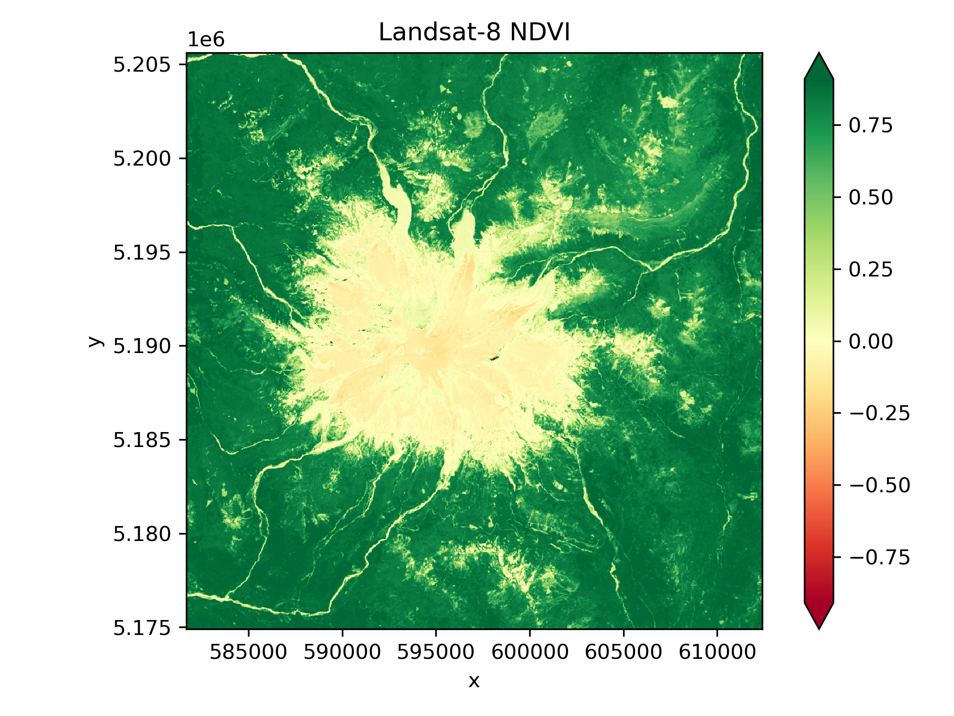
Written response: What differences do you see in NDVI values for dense conifer trees (most of the scene) vs. open meadows or recently logged plots dominated by grass and other deciduous plants?#
STUDENT WRITTEN RESPONSE HERE
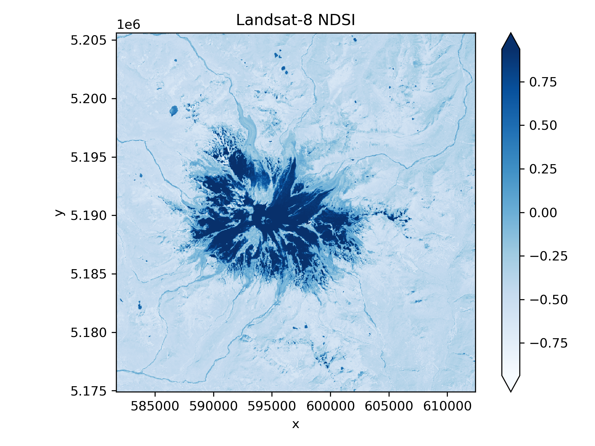
Calculate NDSI (normalized difference snow index), clip values to [-1,1], and plot with robust=True#
# STUDENT CODE HERE
# STUDENT CODE HERE
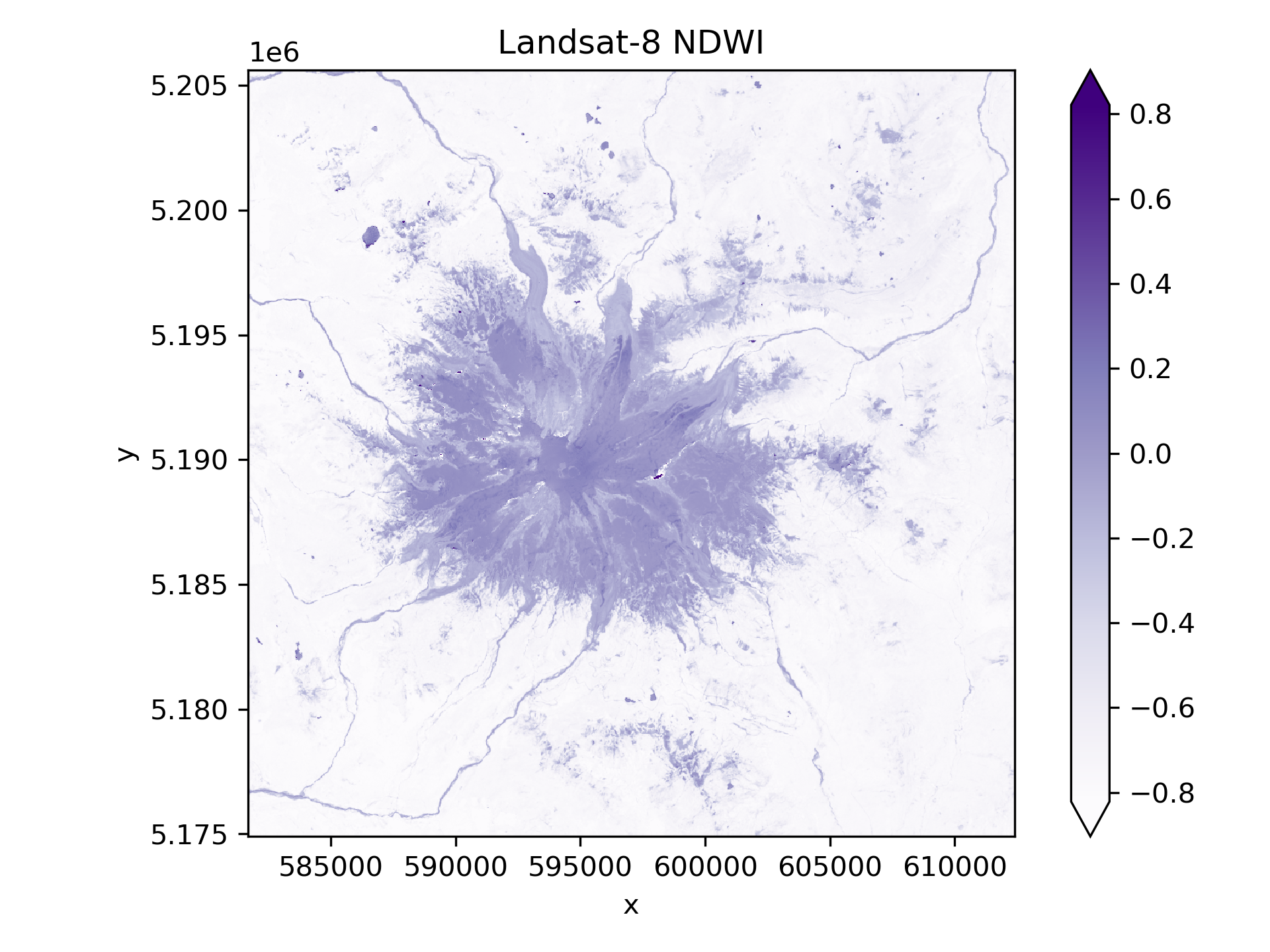
Calculate NDWI (normalized difference water index), clip values to [-1,1], and plot with robust=True#
# STUDENT CODE HERE
# STUDENT CODE HERE
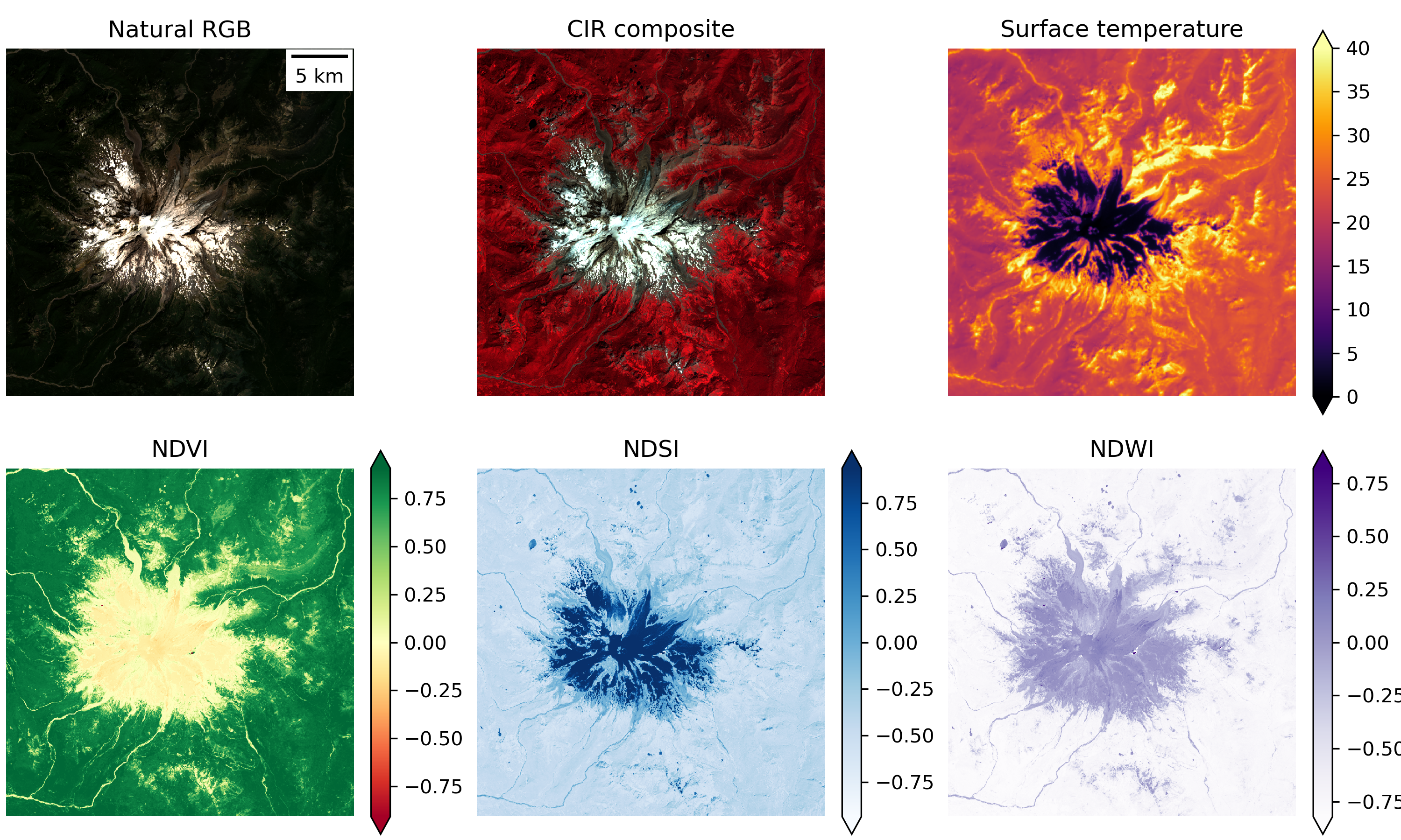
Create a figure with linked RGB, CIR, surface temperature, NDVI, NDSI, and NDWI products#
Add a scalebar on the RGB plot!
Use the pan/zoom functionality of
%matplotlib widgetto explore the scene a bitZoom in on some vegetation, snow near the summit, and surface water like Mowich Lake
When you turn in the lab, make sure the plot is saved as a static plot and not the interactive version
Note how the different indices change (see interactive values for cursor position on each subplot), which should hopefully provide better sense of what the different indices are showing
# STUDENT CODE HERE
Written response: Pan and zoom around interactively. Write about one thing or feature that you found interesting, making sure to incorporate information from at least three of the rasters.#
STUDENT WRITTEN RESPONSE HERE
Part 8: Raster thresholding (2 pts)#
Create a binary vegetation mask#
We need to define a cutoff value (threshold) for NDVI values to define a boolean vegetation mask
NDVI values above this threshold will be classified as “vegetation”
NDVI values below this threshold will be classified as “not vegetation”
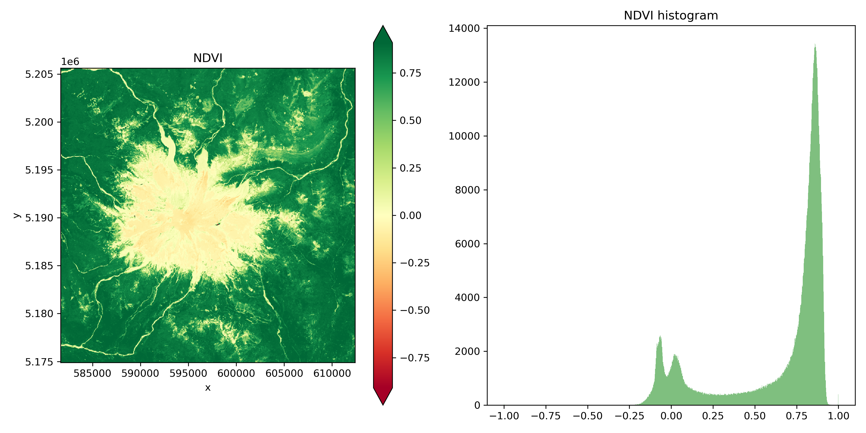
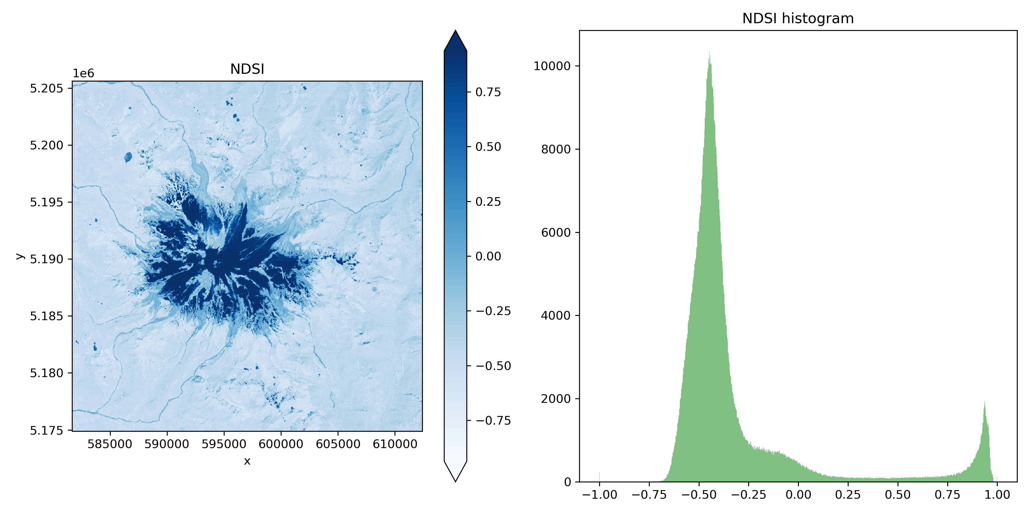
To decide on a threshold, create a figure with an NDVI plot on the left and a histogram of NDVI values on the right#
# STUDENT CODE HERE
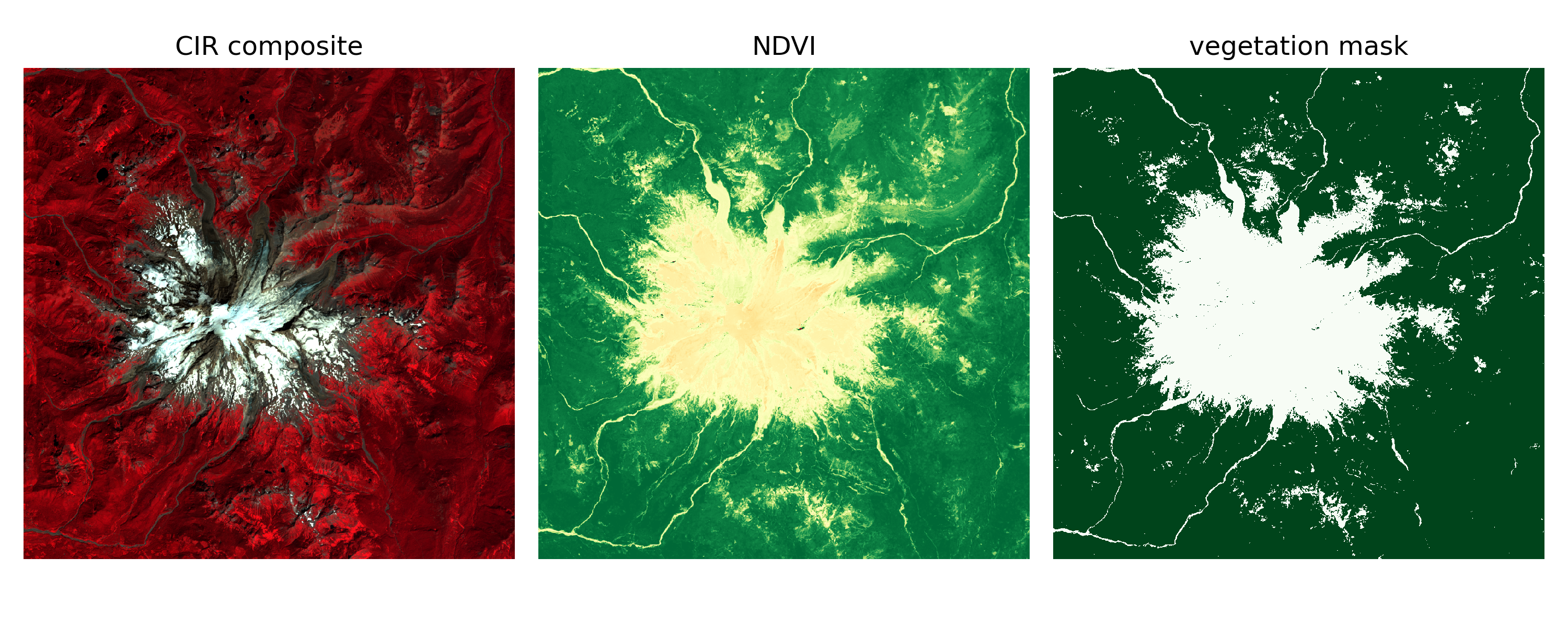
Based on the histogram, choose an NDVI threshold and create a binary vegetation mask. Then create a figure with three subplots: CIR, NDVI, and your new veegtation mask.#
# STUDENT CODE HERE
<xarray.DataArray (y: 1024, x: 1024)> Size: 1MB
array([[ True,  True,  True, ...,  True,  True,  True],
       [ True,  True,  True, ...,  True,  True,  True],
       [ True,  True,  True, ...,  True,  True,  True],
       ...,
       [ True,  True,  True, ...,  True,  True,  True],
       [ True,  True,  True, ...,  True,  True,  True],
       [ True,  True,  True, ...,  True,  True,  True]])
Coordinates:
    band         int64 8B 1
  * x            (x) float64 8kB 5.817e+05 5.817e+05 ... 6.124e+05 6.124e+05
  * y            (y) float64 8kB 5.206e+06 5.206e+06 ... 5.175e+06 5.175e+06
spatial_ref int64 8B 0# STUDENT CODE HERE
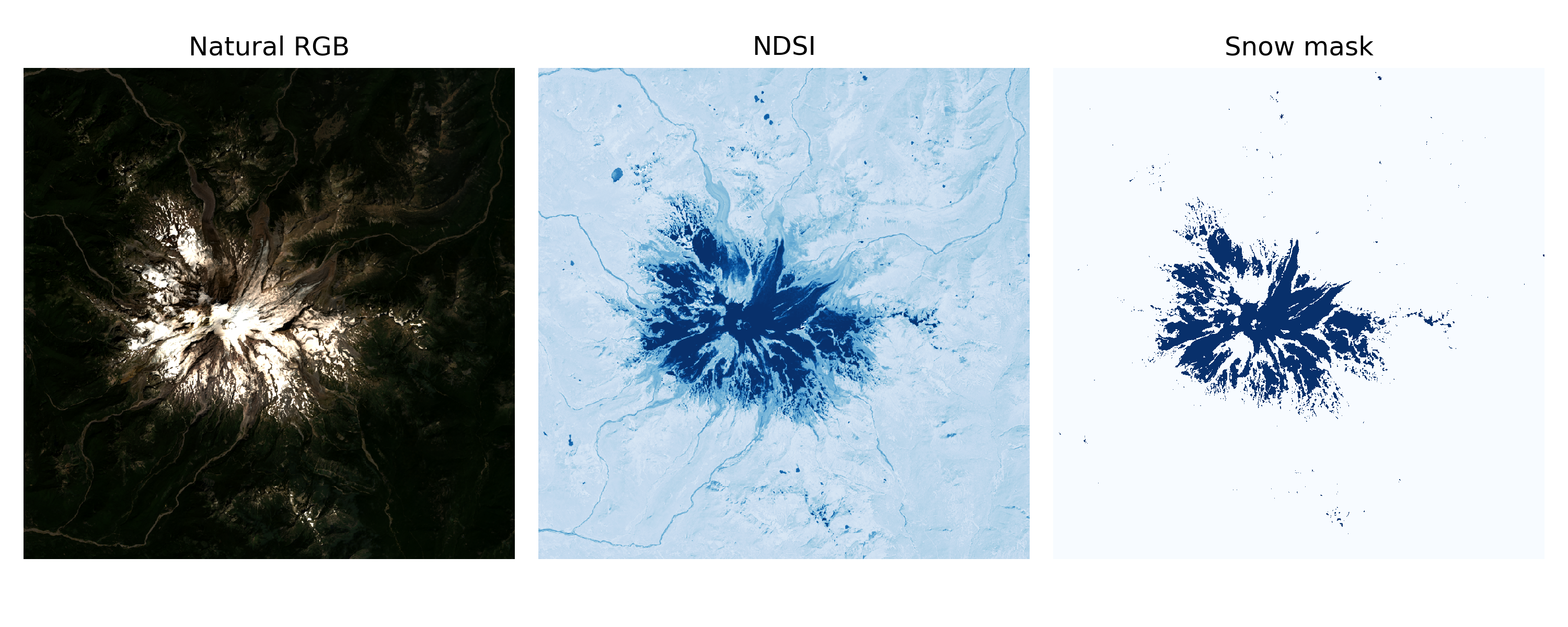
Create a binary snow mask. Then, create a figure with natural RGB, NDSI, and your new binary snow mask#
Follow a similar procedure with thresholding to create a snow mask from NDSI
# STUDENT CODE HERE
# STUDENT CODE HERE
# STUDENT CODE HERE
Part 9: Raster area and change (3 pts)#
Use your snow mask to estimate the area (km2) covered by snow in August and in December#
Bring in the December rasters, creating a natural RGB composite an NDSI image, and a binary snow mask#
Use the same NDSI threshold for both August and December!
# STUDENT CODE HERE
# STUDENT CODE HERE
<xarray.DataArray (y: 1024, x: 1024)> Size: 4MB
array([[-0.12144855, -0.22127382, -0.13928398, ...,  1.        ,
         1.        ,  1.        ],
       [-0.14421098, -0.14118597, -0.03769719, ...,  1.        ,
         1.        , -1.        ],
       [-0.00795951,  0.02210915,  0.01732341, ...,  1.        ,
         1.        ,  1.        ],
       ...,
       [-0.13700016, -0.14488819, -0.13657251, ...,  0.21691905,
         0.2368435 ,  0.38473162],
       [-0.15323447, -0.15313424, -0.15563335, ...,  0.11950976,
         0.19356021,  0.2021742 ],
       [-0.15105893, -0.15632582, -0.1772668 , ...,  0.11733061,
         0.15551701,  0.2443123 ]], dtype=float32)
Coordinates:
    band         int64 8B 1
  * x            (x) float64 8kB 5.817e+05 5.817e+05 ... 6.124e+05 6.124e+05
  * y            (y) float64 8kB 5.206e+06 5.206e+06 ... 5.175e+06 5.175e+06
spatial_ref int64 8B 0# STUDENT CODE HERE
Create a figure with two rows and three columns. The top row should be the August image and bottom row should be the December image. The columns should be natural RGB image, NDSI, and snow mask#
# STUDENT CODE HERE
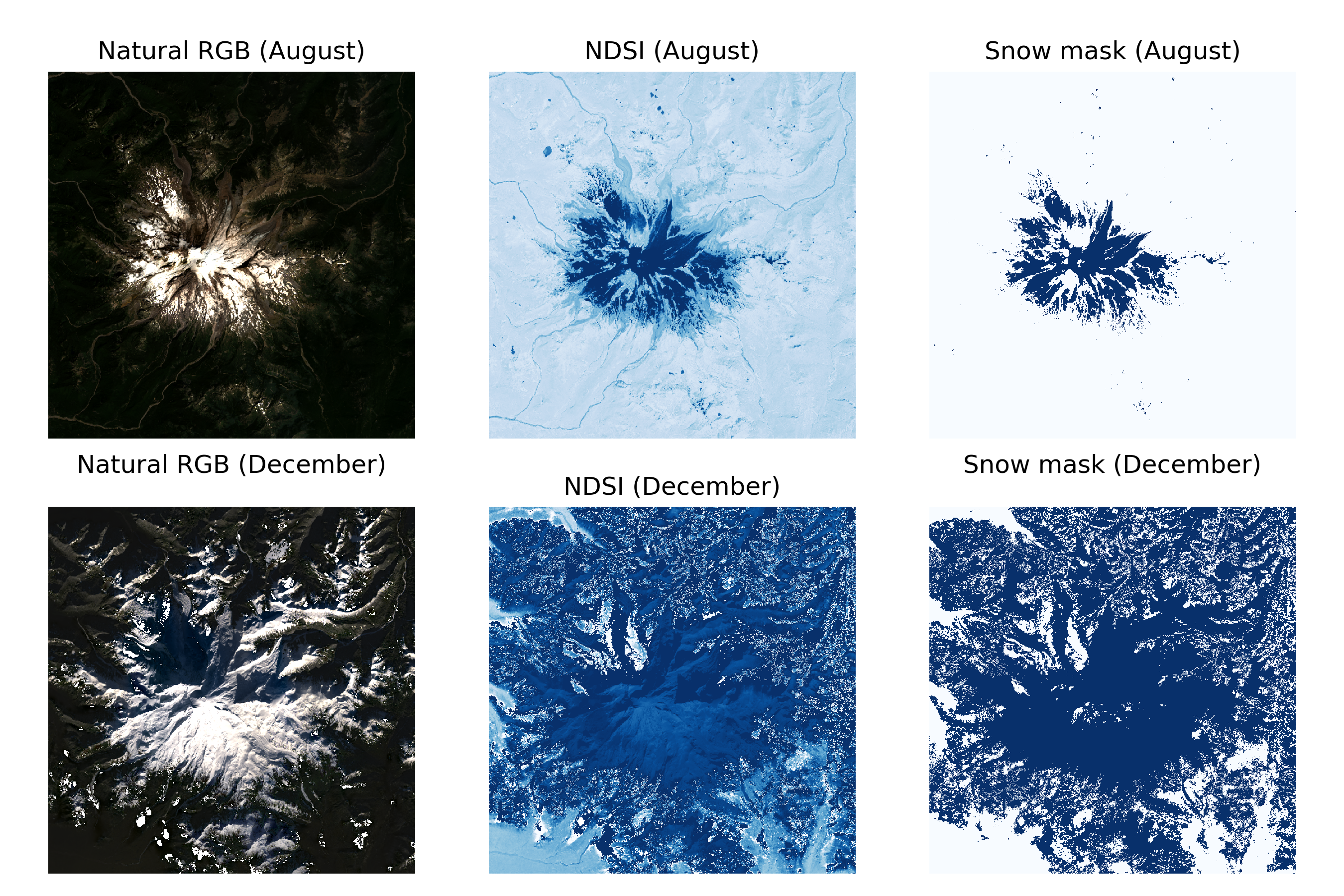
Written response: What do you think is going on in the December image? Why do things look a little strange?#
STUDENT WRITTEN RESPONSE HERE
Calculate the snow extent for both images in km2#
You will need to count the number of snow pixels and multiply by the area of each pixel
Confidence check: look at the RGB image, your snow mask, and estimate the percentage of the windowed area (~31 x 31 km) covered by snow
Hint: Snow-covered area of ~60-70 km2 seems reasonable
Note: Based on what we learned in our earlier lab on CRS/projections, this calculation should really be done using an equal-area projection. Fine to estimate with default UTM projection here–we will cover raster reprojection in the Raster 2 lab.
# STUDENT CODE HERE
# STUDENT CODE HERE
Snow extent in August: 66.13 km^2
Snow extent in December: 672.83 km^2
Submit your work#
Make sure to do this process for both notebooks!
Save this notebook with all code and output (Make sure when you save the notebook, all cells show their outputs).
Use the terminal to stage, commit, and push your notebook to your GitHub repository. It should look something like this…
git add 01_lab.ipynb
git commit -m “Completed Lab 01 exercises”
git push
Verify that your notebook appears in your GitHub repository. Double check to make sure all the ouputs are visible!