Lab 06 assignment (20 pts)#
UW Geospatial Data Analysis
CEE467/CEWA567
David Shean, Eric Gagliano, Quinn Brencher
Introduction#
Objectives#
Continue to explore raster data
Learn strategies for dynamic DEM downloading
Explore raster reprojection, clipping, sampling at points, and zonal statistics
Explore local sea level rise and road hazards using DEMs
Instructions#
For each question or task below, write some code in the empty cell and execute to preserve your output
If you are in the graduate section of the class, please complete at least 2 extra credit problems
Work together, consult resources we’ve discussed, post on slack!
Follow the submission instructions at the end of the lab!
Part 0: Imports and filenames#
First, let’s import the libraries we’ll need. Make sure to shut down any other kernels you have running!#
import os
import requests
import numpy as np
import pandas as pd
import geopandas as gpd
import rasterio as rio
from rasterio import plot, mask
from rasterio.warp import calculate_default_transform, reproject, Resampling
import matplotlib.pyplot as plt
import rasterstats
import rioxarray as rxr
from matplotlib_scalebar.scalebar import ScaleBar
from pathlib import Path
#%matplotlib widget
dem_data = f'{Path.home()}/gda_demo_data/dem_data'
# If you see no output for this cell, run the Jupyterbook demo notebook to query and download data (06_demo.ipynb)
!ls -lh $dem_data
total 813M
-rw-r--r-- 1 eric eric 3.8M Feb  9 13:17 SEA_COP30.tif
-rw-r--r-- 1 eric eric 780K Feb  9 13:17 SEA_SRTMGL1.tif
-rw-r--r-- 1 eric eric 142M Feb  9 13:21 WA_COP90.tif
-rw-r--r-- 1 eric eric 199M Feb  9 14:53 WA_COP90_utm_gdalwarp.tif
-rw-r--r-- 1 eric eric 176M Feb 12 10:45 WA_COP90_utm_gdalwarp_lzw.tif
-rw-r--r-- 1 eric eric  50M Feb 12 10:45 WA_COP90_utm_gdalwarp_lzw_hs.tif
-rw-r--r-- 1 eric eric 199M Feb 12 12:32 WA_COP90_utm_gdalwarp_lzw_slope.tif
-rw-r--r-- 1 eric eric  46M Feb  9 13:20 WA_SRTMGL3.tif
#We will use the Copernicus 90m dataset for these exercises
dem_fn = os.path.join(dem_data, "WA_COP90.tif")
dem_fn
'/home/eric/gda_demo_data/dem_data/WA_COP90.tif'
Part 1: Prepare DEM data (1 pts)#
Reproject the WA DEM data using the command line gdalwarp#
See demo for an example of gdalwarp
We could do this using rioxarray (or even rasterio), but for use cases where we have a file already on disk and we’d like to create another file on disk, gdalwarp is convenient
Output should be LZW compressed and tiled
to account for the fact that the Copernicus DEM doesn’t have a nodata value set in the metadata, pass in
-srcnodata 0
# Define desired CRS for output and filename of the projected raster
dst_crs = 'EPSG:32610'
proj_fn = os.path.splitext(dem_fn)[0]+'_utm_gdalwarp_lzw.tif'
# STUDENT CODE HERE
Prepare the projected data#
Open the raster as
dem_dausing rioxarrayInspect the crs and cofirm this raster is in the correct crs
Use
xarray’s.where()functionality to mask all values less than or equal to 0Do a quick plot to make sure everything looks good
# STUDENT CODE HERE
# STUDENT CODE HERE
# STUDENT CODE HERE
# STUDENT CODE HERE
Using gdaldem as we did in the demo, create a shaded relief map for the projected DEM#
# Define desired output filename of the hillshade raster
hs_fn = os.path.splitext(proj_fn)[0]+'_hs.tif'
# STUDENT CODE HERE
Now load the hillshade raster you just created as hs_da using rioxarray#
# STUDENT CODE HERE
<xarray.DataArray (y: 5851, x: 8877)> Size: 208MB
[51939327 values with dtype=float32]
Coordinates:
    band         int64 8B 1
  * x            (x) float64 71kB 3.647e+05 3.648e+05 ... 9.748e+05 9.749e+05
  * y            (y) float64 47kB 5.446e+06 5.446e+06 ... 5.043e+06 5.043e+06
    spatial_ref  int64 8B 0
Attributes:
    AREA_OR_POINT:  Area
    scale_factor:   1.0
add_offset: 0.0Prepare the states geodataframe#
We’ve created
states_gdffor youNow create
states_proj_gdf, which is the states_gdf reprojected todem_da’s crsFinally create
wa_state_gdf, a geodataframe of just the Washington row
#states_url = 'http://eric.clst.org/assets/wiki/uploads/Stuff/gz_2010_us_040_00_5m.json'
states_url = 'http://eric.clst.org/assets/wiki/uploads/Stuff/gz_2010_us_040_00_500k.json'
states_gdf = gpd.read_file(states_url)
states_gdf
| GEO_ID | STATE | NAME | LSAD | CENSUSAREA | geometry | |
|---|---|---|---|---|---|---|
| 0 | 0400000US23 | 23 | Maine | 30842.923 | MULTIPOLYGON (((-67.61976 44.51975, -67.61541 ... | |
| 1 | 0400000US25 | 25 | Massachusetts | 7800.058 | MULTIPOLYGON (((-70.83204 41.6065, -70.82374 4... | |
| 2 | 0400000US26 | 26 | Michigan | 56538.901 | MULTIPOLYGON (((-88.68443 48.11578, -88.67563 ... | |
| 3 | 0400000US30 | 30 | Montana | 145545.801 | POLYGON ((-104.0577 44.99743, -104.25014 44.99... | |
| 4 | 0400000US32 | 32 | Nevada | 109781.180 | POLYGON ((-114.0506 37.0004, -114.05 36.95777,... | |
| 5 | 0400000US34 | 34 | New Jersey | 7354.220 | POLYGON ((-75.52684 39.65571, -75.52634 39.656... | |
| 6 | 0400000US36 | 36 | New York | 47126.399 | MULTIPOLYGON (((-71.94356 41.28668, -71.9268 4... | |
| 7 | 0400000US37 | 37 | North Carolina | 48617.905 | MULTIPOLYGON (((-82.60288 36.03983, -82.60074 ... | |
| 8 | 0400000US39 | 39 | Ohio | 40860.694 | MULTIPOLYGON (((-82.81349 41.72347, -82.81049 ... | |
| 9 | 0400000US42 | 42 | Pennsylvania | 44742.703 | POLYGON ((-75.41504 39.80179, -75.42804 39.809... | |
| 10 | 0400000US44 | 44 | Rhode Island | 1033.814 | MULTIPOLYGON (((-71.28157 41.64821, -71.27817 ... | |
| 11 | 0400000US47 | 47 | Tennessee | 41234.896 | POLYGON ((-81.67754 36.58812, -81.68014 36.585... | |
| 12 | 0400000US48 | 48 | Texas | 261231.711 | MULTIPOLYGON (((-97.13436 27.89633, -97.1336 2... | |
| 13 | 0400000US49 | 49 | Utah | 82169.620 | POLYGON ((-114.0506 37.0004, -114.05175 37.088... | |
| 14 | 0400000US53 | 53 | Washington | 66455.521 | MULTIPOLYGON (((-123.09055 49.00198, -123.0353... | |
| 15 | 0400000US55 | 55 | Wisconsin | 54157.805 | MULTIPOLYGON (((-90.45525 47.024, -90.45713 47... | |
| 16 | 0400000US72 | 72 | Puerto Rico | 3423.775 | MULTIPOLYGON (((-65.58734 18.38199, -65.59122 ... | |
| 17 | 0400000US24 | 24 | Maryland | 9707.241 | MULTIPOLYGON (((-76.07147 38.2035, -76.04879 3... | |
| 18 | 0400000US01 | 01 | Alabama | 50645.326 | MULTIPOLYGON (((-85.00237 31.00068, -85.02411 ... | |
| 19 | 0400000US02 | 02 | Alaska | 570640.950 | MULTIPOLYGON (((-164.9762 54.1346, -164.93777 ... | |
| 20 | 0400000US04 | 04 | Arizona | 113594.084 | POLYGON ((-109.04522 36.99908, -109.04524 36.9... | |
| 21 | 0400000US05 | 05 | Arkansas | 52035.477 | POLYGON ((-94.55929 36.4995, -94.51948 36.4992... | |
| 22 | 0400000US06 | 06 | California | 155779.220 | MULTIPOLYGON (((-122.44632 37.86105, -122.4385... | |
| 23 | 0400000US08 | 08 | Colorado | 103641.888 | POLYGON ((-102.04224 36.99308, -102.0545 36.99... | |
| 24 | 0400000US09 | 09 | Connecticut | 4842.355 | MULTIPOLYGON (((-71.85957 41.3224, -71.86824 4... | |
| 25 | 0400000US10 | 10 | Delaware | 1948.543 | MULTIPOLYGON (((-75.55945 39.62981, -75.5591 3... | |
| 26 | 0400000US11 | 11 | District of Columbia | 61.048 | POLYGON ((-77.0386 38.79151, -77.0389 38.80081... | |
| 27 | 0400000US12 | 12 | Florida | 53624.759 | MULTIPOLYGON (((-85.15642 29.67963, -85.1374 2... | |
| 28 | 0400000US13 | 13 | Georgia | 57513.485 | POLYGON ((-81.44412 30.70971, -81.44872 30.709... | |
| 29 | 0400000US15 | 15 | Hawaii | 6422.628 | MULTIPOLYGON (((-171.73761 25.7921, -171.72237... | |
| 30 | 0400000US16 | 16 | Idaho | 82643.117 | POLYGON ((-111.04669 42.00157, -111.41587 42.0... | |
| 31 | 0400000US17 | 17 | Illinois | 55518.930 | POLYGON ((-87.53233 39.99778, -87.53254 39.987... | |
| 32 | 0400000US18 | 18 | Indiana | 35826.109 | POLYGON ((-88.02803 37.79922, -88.02938 37.803... | |
| 33 | 0400000US19 | 19 | Iowa | 55857.130 | POLYGON ((-95.76564 40.58521, -95.7589 40.5889... | |
| 34 | 0400000US20 | 20 | Kansas | 81758.717 | POLYGON ((-94.61808 36.99814, -94.62522 36.998... | |
| 35 | 0400000US21 | 21 | Kentucky | 39486.338 | MULTIPOLYGON (((-83.67541 36.60081, -83.67561 ... | |
| 36 | 0400000US22 | 22 | Louisiana | 43203.905 | MULTIPOLYGON (((-88.86507 29.75271, -88.88976 ... | |
| 37 | 0400000US27 | 27 | Minnesota | 79626.743 | POLYGON ((-91.37161 43.50094, -91.37695 43.500... | |
| 38 | 0400000US28 | 28 | Mississippi | 46923.274 | MULTIPOLYGON (((-88.71072 30.2508, -88.6568 30... | |
| 39 | 0400000US29 | 29 | Missouri | 68741.522 | POLYGON ((-89.5391 36.4982, -89.53452 36.49143... | |
| 40 | 0400000US31 | 31 | Nebraska | 76824.171 | POLYGON ((-95.76564 40.58521, -95.76853 40.583... | |
| 41 | 0400000US33 | 33 | New Hampshire | 8952.651 | MULTIPOLYGON (((-72.45852 42.72685, -72.45849 ... | |
| 42 | 0400000US35 | 35 | New Mexico | 121298.148 | POLYGON ((-109.05004 31.3325, -109.05017 31.48... | |
| 43 | 0400000US38 | 38 | North Dakota | 69000.798 | POLYGON ((-96.56328 45.93524, -96.5769 45.9352... | |
| 44 | 0400000US40 | 40 | Oklahoma | 68594.921 | POLYGON ((-94.61792 36.49941, -94.61531 36.484... | |
| 45 | 0400000US41 | 41 | Oregon | 95988.013 | POLYGON ((-117.22007 44.30138, -117.22245 44.2... | |
| 46 | 0400000US45 | 45 | South Carolina | 30060.696 | POLYGON ((-78.54109 33.85111, -78.55394 33.847... | |
| 47 | 0400000US46 | 46 | South Dakota | 75811.000 | POLYGON ((-96.44341 42.4895, -96.45971 42.4860... | |
| 48 | 0400000US50 | 50 | Vermont | 9216.657 | POLYGON ((-72.04008 44.15575, -72.04271 44.152... | |
| 49 | 0400000US51 | 51 | Virginia | 39490.086 | MULTIPOLYGON (((-76.04653 37.95359, -76.04169 ... | |
| 50 | 0400000US54 | 54 | West Virginia | 24038.210 | POLYGON ((-81.9683 37.5378, -81.9654 37.54117,... | |
| 51 | 0400000US56 | 56 | Wyoming | 97093.141 | POLYGON ((-109.05008 41.00066, -109.17368 41.0... |
# STUDENT CODE HERE
# STUDENT CODE HERE
| GEO_ID | STATE | NAME | LSAD | CENSUSAREA | geometry | |
|---|---|---|---|---|---|---|
| 14 | 0400000US53 | 53 | Washington | 66455.521 | MULTIPOLYGON (((493377.499 5427679.393, 497411... |
Use rioxarray’s .clip() to clip the dem_da to a WA state dataarray wa_dem_da#
Check out the documentation for the
.clip()function here
# STUDENT CODE HERE
<xarray.DataArray (y: 5832, x: 8727)> Size: 204MB
array([[nan, nan, nan, ..., nan, nan, nan],
[nan, nan, nan, ..., nan, nan, nan],
[nan, nan, nan, ..., nan, nan, nan],
...,
[nan, nan, nan, ..., nan, nan, nan],
[nan, nan, nan, ..., nan, nan, nan],
[nan, nan, nan, ..., nan, nan, nan]], dtype=float32)
Coordinates:
band int64 8B 1
* x (x) float64 70kB 3.711e+05 3.712e+05 ... 9.71e+05 9.71e+05
* y (y) float64 47kB 5.445e+06 5.444e+06 ... 5.044e+06 5.044e+06
spatial_ref int64 8B 0
Attributes:
AREA_OR_POINT: Point
scale_factor: 1.0
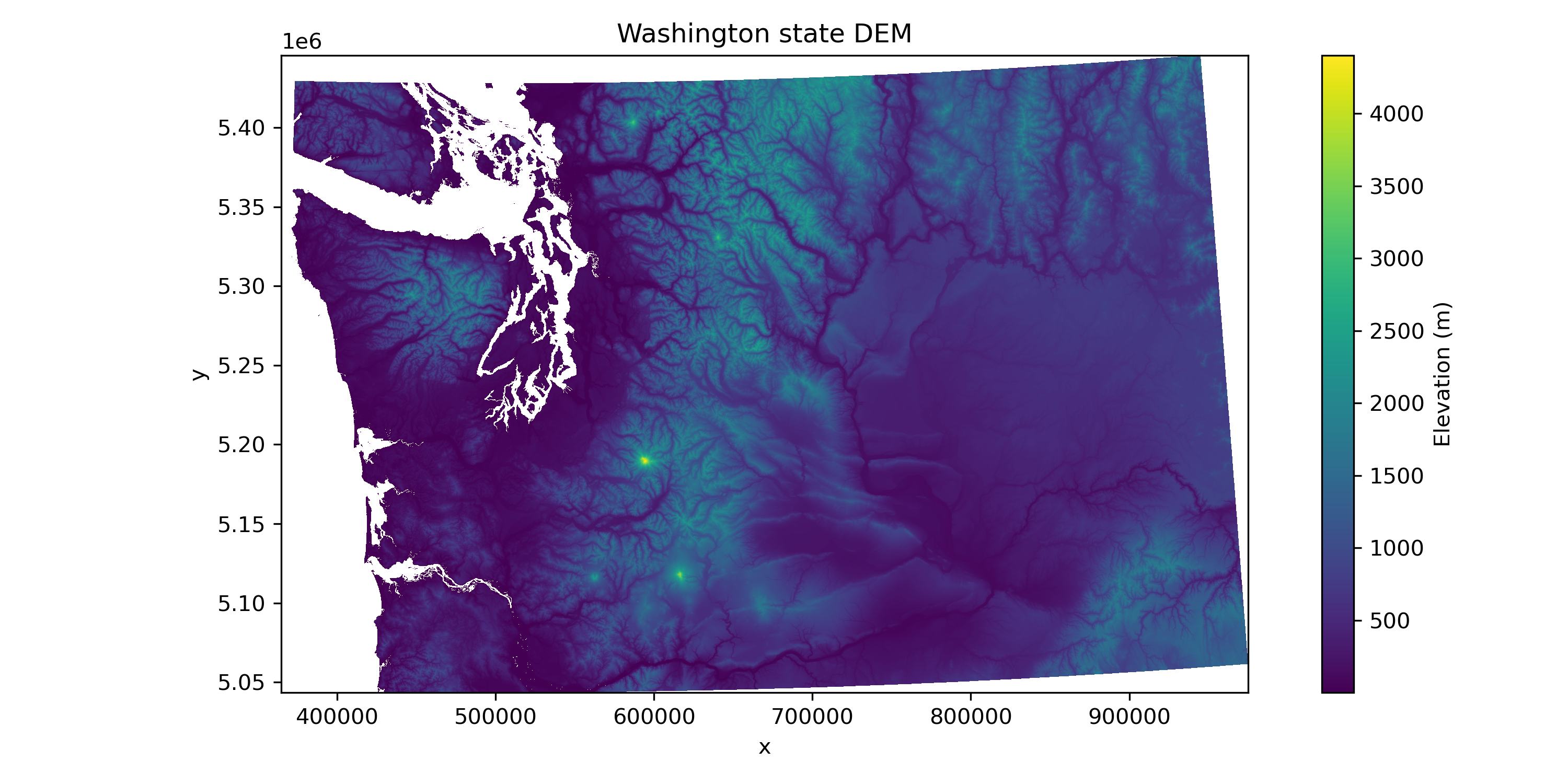
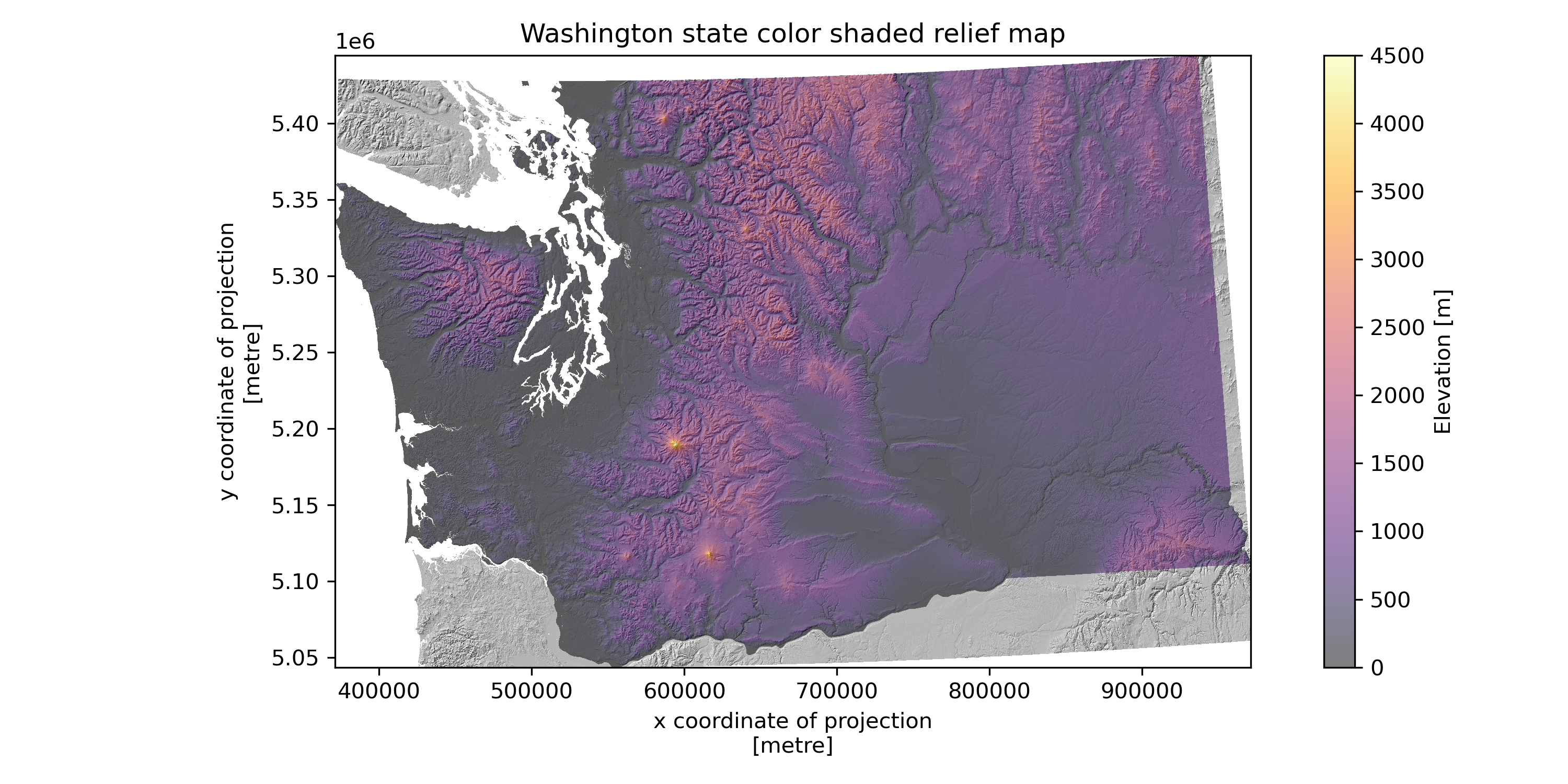
add_offset: 0.0Part 2: DEM visualization and basic analysis (4 pts)#
Create a color shaded relief map#
You should already have the projected, clipped DEM (
wa_dem_da) and the hillshade created from the projected, unclipped DEM (hs_da)Create a plot overlaying color elevation values on the hillshade
either be mindful of the order that you call these plots, or learn about
zorderhere and pass it in to your.imshow()callUse the
alphaargument toimshow()to set transparency of the DEMAdd a colorbar only for the DEM
# STUDENT CODE HERE
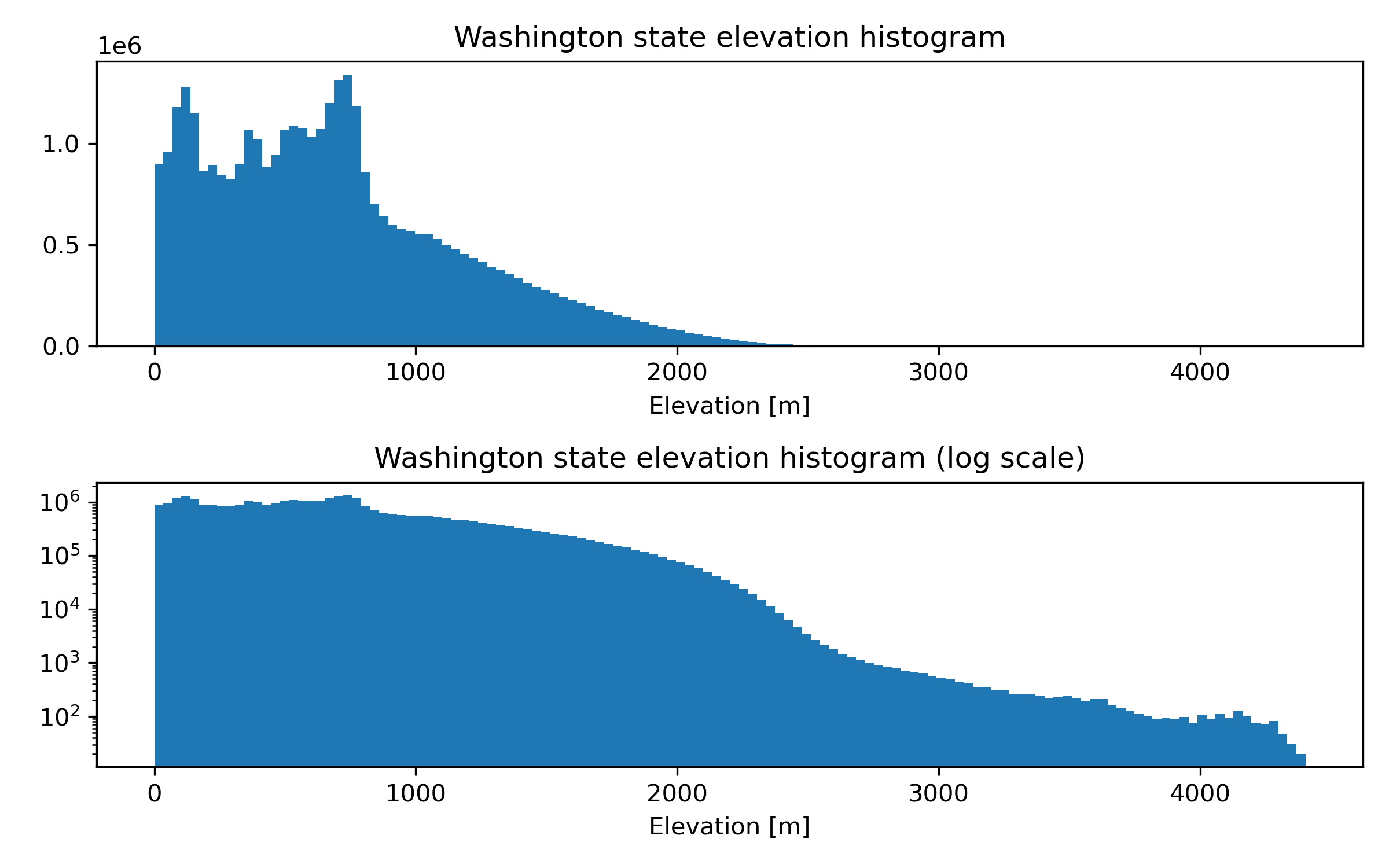
Create a figure with two histograms of elevation values (one regular scale, and another log scale). According to your clipped DEM, What is the maximum elevation in WA state? Use f string formatting to report your results with 2 decmials of precision.#
# STUDENT CODE HERE
# STUDENT CODE HERE
Written response: Look up the maximum elevation of Washington state. How do these values compare, and if they are different, why do you think this is?#
STUDENT WRITTEN RESPONSE HERE
Create a figure for Washington state with an elevation histogram and a binary map of areas above 1 mile (1) and below 1 mile (0). What percentage of Washington state is >1 mile above sea level?#
Make sure to pay attention to units :)
Think back to lab04 and the NDSI threshold approach to determine snow-covered area
Remember, that you have a regular grid here where each pixel is approximately the same dimensions on the ground
After you’ve calculated a binary map, remove the pixels outside of the Washington geometry to avoid inflating the total number of pixels in Washington
As we know, this kind of calculation should be done in an equal-area projection, but fine to estimate with UTM projection here
# STUDENT CODE HERE
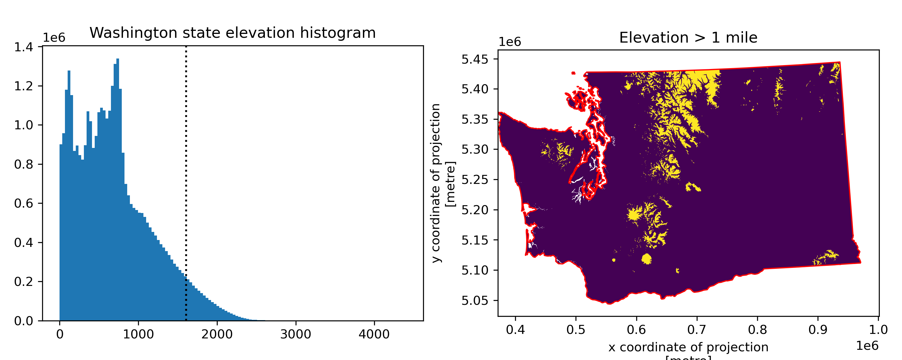
# STUDENT CODE HERE
Part 3: Volume estimation of Whidbey Island (8 pts)#
In the Raster 1 lab, we computed snow-covered area from a 2D array with known pixel dimensions (30x30 m for Landsat-8)
Now, let’s add a third dimension to compute volume from a 2D array of elevation values
Imagine dividing the domain up into 1 cubic meter blocks - your elevation values are like stacks of these 1-m cubes above some reference datum
Volume (and volume change) calculations are common operations with gridded DEMs. The analysis is often referred to as “cut/fill”. For example:
Measuring quarry slag pile volume
Measuring ice sheet and glacier change
Now we’d like to do this for Whidbey Island…
Clip our DEM to the Whidbey Island geometry#
First, extract the Whidbey Island polygon from the WA state geometry to have an area over which to compute volume. We done this for you!
Then clip the DEM by the Whidbey Island geometry
whidbey_gdf = gpd.GeoDataFrame(geometry=gpd.GeoSeries(wa_state_gdf.geometry.iloc[0].geoms[7]),crs=wa_state_gdf.crs)
whidbey_gdf
| geometry | |
|---|---|
| 0 | POLYGON ((535640.328 5348457.49, 535403.34 534... |
# STUDENT CODE HERE
<xarray.DataArray (y: 819, x: 458)> Size: 2MB
array([[nan, nan, nan, ..., nan, nan, nan],
       [nan, nan, nan, ..., nan, nan, nan],
       [nan, nan, nan, ..., nan, nan, nan],
       ...,
       [nan, nan, nan, ..., nan, nan, nan],
       [nan, nan, nan, ..., nan, nan, nan],
       [nan, nan, nan, ..., nan, nan, nan]], dtype=float32)
Coordinates:
band int64 8B 1
* x (x) float64 4kB 5.171e+05 5.172e+05 ... 5.485e+05 5.485e+05
* y (y) float64 7kB 5.362e+06 5.362e+06 ... 5.306e+06 5.306e+06
spatial_ref int64 8B 0
Attributes:
AREA_OR_POINT: Point
scale_factor: 1.0
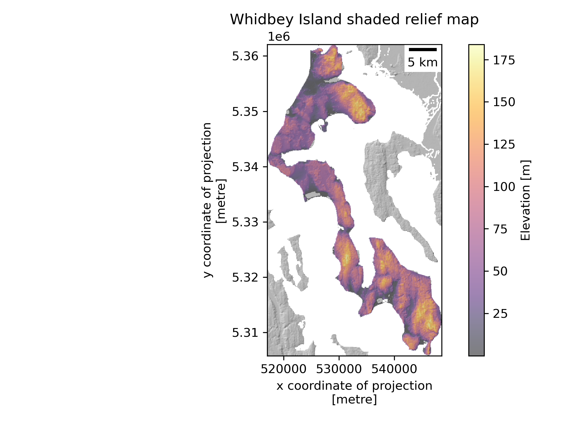
add_offset: 0.0Create a shaded relief map of the clipped Whidbey DEM#
Make sure there is a colorbar and scalebar
# STUDENT CODE HERE
Here we’ll define a “bottom” surface for our volume calculation#
Let’s use a constant elevation above the geoid (mean sea level) as our “baseline” elevation
Since our DEM values are height above the EGM96 geoid, we can use 0 here
Note that this bottom surface can also be more complex: a planar fit to elevations around a polygon, lake bathymetry, etc.
baseline_elev = 0
Compute the area and volume of Whidbey Island#
Compute the height of the DEM above this “baseline” elevation
Do this by calculating the area of Whidbey using the known pixel size (remember
.rio.resolution()fromrioxarray) and pixel count, then multiply by the average height to get volumeConvert the total volume to km^3
# STUDENT CODE HERE
# STUDENT CODE HERE
We’re gonna need a bigger boat…#
Sea level rise is very real
Current global average rates are ~3.6 mm/yr
This may not sound like much, but over 100 years, thats 36 cm or ~1.2 feet! And the rate is increasing nonlinearly.
Some good references:
U.S. Interagency report from 2022: https://oceanservice.noaa.gov/hazards/sealevelrise/sealevelrise-tech-report.html
https://www.ipcc.ch/srocc/chapter/chapter-4-sea-level-rise-and-implications-for-low-lying-islands-coasts-and-communities/
https://archive.ipcc.ch/publications_and_data/ar4/wg1/en/faq-5-1.html
https://www.ipcc.ch/site/assets/uploads/2018/02/WG1AR5_Chapter13_FINAL.pdf
http://www.antarcticglaciers.org/glaciers-and-climate/what-is-the-global-volume-of-land-ice-and-how-is-it-changing/
Let’s do some rough inundation calculations using our DEM
Note that in practice, we wouldn’t use a global DEM product like SRTM or COP30 for this, but would use a very accurate airborne lidar datset (like the most recent lidar data available from USGS 3DEP or WA DNR)
There are many other caveats here, as sea level rise is much more complex than just “filling the bathtub” (see the IPCC report), but we’re learning concepts and techniques, so let’s start with a simple case.
Create a function to compute the area and volume of whidbey island above sea level for the following…#
1 meter of sea level rise
10 meters of sea level rise
20 meters of sea level rise
66 meters of sea level rise (roughly the total if all land ice melted, without accounting for thermal expansion)
Add a visualization component to your function#
Create plots using the Whidbey Polygon as “reference shoreline”, and plot valid DEM values above the sea level with fixed color ramp limits
Add notation for area and volume above sea level
#def slr_plot(dem_ma, sl=0):
# STUDENT CODE HERE
slr_values = (0,1,10,20,66)
for i in slr_values:
    slr_plot(whidbey_dem_da, sl=i)


Challenge question: Create area and volume inundation curves (GS: Attempt required / UG: +1 pts)#
Starting with sea level of 0, increase by 1 m increments until Whidbey is totally submerged
Create plots for:
exposed area vs sea level
exposed volume vs sea level
# STUDENT CODE HERE
# STUDENT CODE HERE
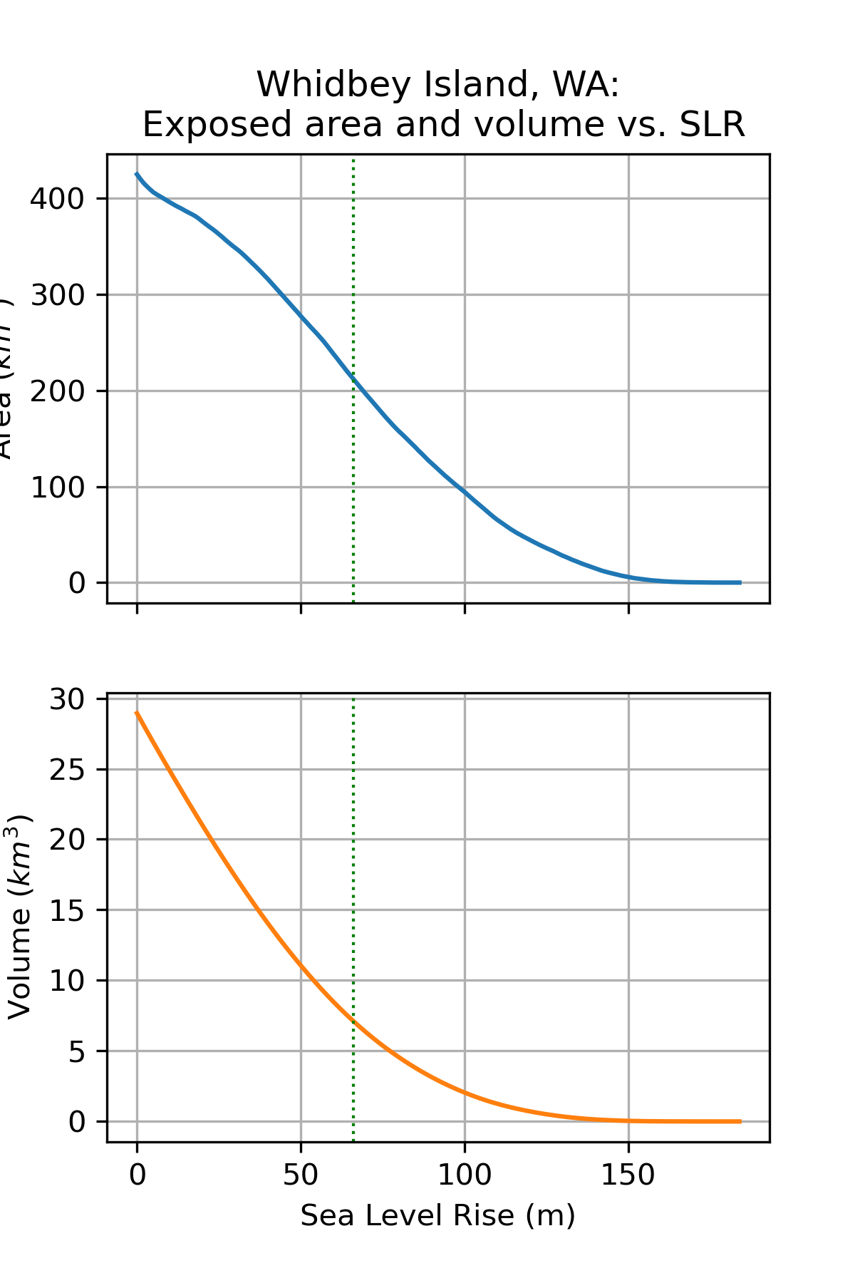
Written response: Whether you did the previous question or not, please take a look at the example output. Are these curves linear? When is the incrimental area loss the greatest? Now take a look at this website and enter a sea level rise level we looked at. In the future, where in the world do you think people will be most affected by sea level rise?#
STUDENT WRITTEN RESPONSE HERE
Part 4: Sampling rasters with geometries (3 pts)#
We saw in lab 4 how we can sample points from rasters easily using xarray. Now we’d like to use geometries to sample rasters! For instance, we could look at the other islands in Washington to see which has the highest mean elevation, or highest elevation variability. We’ve created a geodataframe for you of the Washington state islands, and have added an area column. Note that these don’t have island names attached!
wa_islands_gdf = gpd.GeoDataFrame(geometry=gpd.GeoSeries(wa_state_gdf.geometry.iloc[0].geoms),crs=wa_state_gdf.crs)
wa_islands_gdf.drop(8,inplace=True) # dropping the large WA geometry so we are just focusing on islands
wa_islands_gdf["area"] = wa_islands_gdf.area/1E6
wa_islands_gdf
| geometry | area | |
|---|---|---|
| 0 | POLYGON ((493377.499 5427679.393, 497411.378 5... | 12.369752 |
| 1 | POLYGON ((498125.387 5396104.484, 498551.144 5... | 12.980913 |
| 2 | POLYGON ((522358.867 5398294.937, 524355.92 53... | 24.253250 |
| 3 | POLYGON ((522162.791 5385381.969, 522250.804 5... | 4.001026 |
| 4 | POLYGON ((521044.354 5384006.526, 522512.242 5... | 24.361715 |
| 5 | POLYGON ((525853.989 5381767.464, 526356.093 5... | 21.914111 |
| 6 | POLYGON ((550576.904 5318743.139, 551953.366 5... | 1.765456 |
| 7 | POLYGON ((535640.328 5348457.49, 535403.34 534... | 448.596553 |
| 9 | POLYGON ((503819.099 5403118.917, 502354.404 5... | 1.226159 |
| 10 | POLYGON ((507586.836 5399225.791, 505614.976 5... | 6.176774 |
| 11 | POLYGON ((512438.978 5398928.77, 511275.607 53... | 0.884280 |
| 12 | POLYGON ((517890.167 5393548, 516422.885 53936... | 1.513438 |
| 13 | POLYGON ((490383.028 5389193.184, 490003.51 53... | 14.167604 |
| 14 | POLYGON ((530936.449 5388051.768, 530655.733 5... | 0.853965 |
| 15 | POLYGON ((492252.922 5386706.68, 491265.27 538... | 2.402406 |
| 16 | POLYGON ((496675.778 5384040.205, 496150.164 5... | 1.110354 |
| 17 | POLYGON ((529284.001 5383655.741, 528687.031 5... | 1.036148 |
| 18 | POLYGON ((508430.842 5381665.095, 507553.52 53... | 165.044560 |
| 19 | POLYGON ((509418.745 5362769.935, 507745.73 53... | 108.777328 |
| 20 | POLYGON ((503647.136 5329414.619, 505275.143 5... | 1.776146 |
| 21 | POLYGON ((538729.495 5264055.844, 537876.854 5... | 2.277689 |
| 22 | POLYGON ((538297.255 5241989.66, 537406.38 524... | 107.700866 |
| 23 | POLYGON ((512253.499 5233545.804, 511964.915 5... | 1.538207 |
| 24 | POLYGON ((529644.08 5229343.435, 529418.163 52... | 15.684670 |
| 25 | POLYGON ((524296.578 5226344.363, 523258.677 5... | 19.288300 |
| 26 | POLYGON ((527360.963 5221485.387, 527324.008 5... | 1.125969 |
| 27 | POLYGON ((522657.002 5219065.67, 521843.295 52... | 24.010880 |
| 28 | POLYGON ((513144.601 5381652, 513143.798 53819... | 1.004253 |
| 29 | POLYGON ((503731.605 5376951.972, 502537.119 5... | 24.320284 |
| 30 | POLYGON ((514197.833 5375375.055, 513537.632 5... | 18.301091 |
| 31 | POLYGON ((533413.116 5374116.616, 533020.855 5... | 0.547263 |
| 32 | POLYGON ((502594.587 5366267.175, 498416.077 5... | 171.396513 |
Plot the WA island geometries on top of a shaded relief map#
You can set your xlims and ylims to
ax.set_xlim([480000,560000])andax.set_ylim([5200000,5420000])
# STUDENT CODE HERE
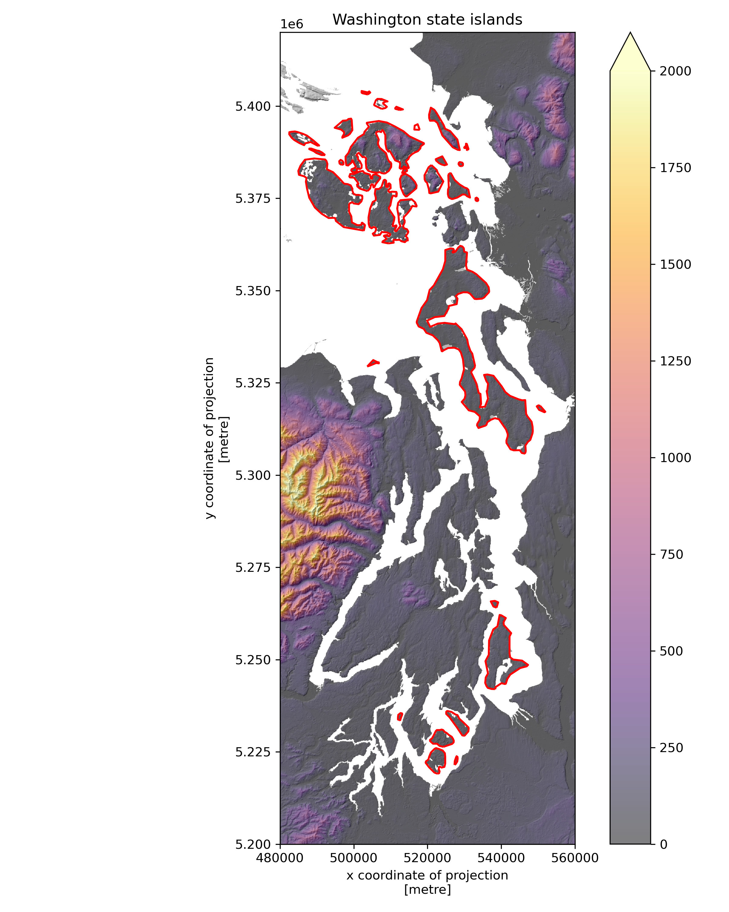
Add elevation_mean and elevation_std columns to the geodataframe#
Hint: one possible method would loop through the geodataframe, clip the DEM by that row’s geometry, use xarray’s builtin mean and std functions, and add these values to the geodataframe
# STUDENT CODE HERE
| geometry | area | elevation_mean | elevation_std | |
|---|---|---|---|---|
| 0 | POLYGON ((493377.499 5427679.393, 497411.378 5... | 12.369752 | 42.598793 | 25.707930 |
| 1 | POLYGON ((498125.387 5396104.484, 498551.144 5... | 12.980913 | 60.742802 | 37.345104 |
| 2 | POLYGON ((522358.867 5398294.937, 524355.92 53... | 24.253250 | 150.514313 | 136.826019 |
| 3 | POLYGON ((522162.791 5385381.969, 522250.804 5... | 4.001026 | 32.318024 | 15.352254 |
| 4 | POLYGON ((521044.354 5384006.526, 522512.242 5... | 24.361715 | 194.967041 | 120.928894 |
| 5 | POLYGON ((525853.989 5381767.464, 526356.093 5... | 21.914111 | 48.657471 | 31.647987 |
| 6 | POLYGON ((550576.904 5318743.139, 551953.366 5... | 1.765456 | 56.812164 | 17.463062 |
| 7 | POLYGON ((535640.328 5348457.49, 535403.34 534... | 448.596553 | 68.084488 | 38.189163 |
| 9 | POLYGON ((503819.099 5403118.917, 502354.404 5... | 1.226159 | 29.336145 | 10.363745 |
| 10 | POLYGON ((507586.836 5399225.791, 505614.976 5... | 6.176774 | 34.927296 | 16.215761 |
| 11 | POLYGON ((512438.978 5398928.77, 511275.607 53... | 0.884280 | 39.506493 | 15.666217 |
| 12 | POLYGON ((517890.167 5393548, 516422.885 53936... | 1.513438 | 22.130949 | 9.321194 |
| 13 | POLYGON ((490383.028 5389193.184, 490003.51 53... | 14.167604 | 58.779362 | 38.645962 |
| 14 | POLYGON ((530936.449 5388051.768, 530655.733 5... | 0.853965 | 17.524363 | 14.278227 |
| 15 | POLYGON ((492252.922 5386706.68, 491265.27 538... | 2.402406 | 60.271034 | 27.545017 |
| 16 | POLYGON ((496675.778 5384040.205, 496150.164 5... | 1.110354 | 37.016724 | 15.710987 |
| 17 | POLYGON ((529284.001 5383655.741, 528687.031 5... | 1.036148 | 62.753143 | 24.030741 |
| 18 | POLYGON ((508430.842 5381665.095, 507553.52 53... | 165.044560 | 163.602722 | 149.080841 |
| 19 | POLYGON ((509418.745 5362769.935, 507745.73 53... | 108.777328 | 52.280388 | 29.445436 |
| 20 | POLYGON ((503647.136 5329414.619, 505275.143 5... | 1.776146 | 33.330933 | 16.564713 |
| 21 | POLYGON ((538729.495 5264055.844, 537876.854 5... | 2.277689 | 56.900578 | 22.883148 |
| 22 | POLYGON ((538297.255 5241989.66, 537406.38 524... | 107.700866 | 90.965004 | 34.575779 |
| 23 | POLYGON ((512253.499 5233545.804, 511964.915 5... | 1.538207 | 31.836172 | 12.931045 |
| 24 | POLYGON ((529644.08 5229343.435, 529418.163 52... | 15.684670 | 56.701618 | 31.367323 |
| 25 | POLYGON ((524296.578 5226344.363, 523258.677 5... | 19.288300 | 50.673149 | 24.446152 |
| 26 | POLYGON ((527360.963 5221485.387, 527324.008 5... | 1.125969 | 52.720879 | 23.880995 |
| 27 | POLYGON ((522657.002 5219065.67, 521843.295 52... | 24.010880 | 52.762386 | 25.759649 |
| 28 | POLYGON ((513144.601 5381652, 513143.798 53819... | 1.004253 | 56.699722 | 23.412815 |
| 29 | POLYGON ((503731.605 5376951.972, 502537.119 5... | 24.320284 | 53.258434 | 25.885468 |
| 30 | POLYGON ((514197.833 5375375.055, 513537.632 5... | 18.301091 | 153.137070 | 68.956070 |
| 31 | POLYGON ((533413.116 5374116.616, 533020.855 5... | 0.547263 | 78.034897 | 18.919979 |
| 32 | POLYGON ((502594.587 5366267.175, 498416.077 5... | 171.396513 | 66.536835 | 51.232857 |
Written response: Which island has the highest mean elevation? What about the greatest standard deviation? For the island with the highest standard deviation, please plot it and try to figure out the islands name using its shape and location.#
STUDENT WRITTEN RESPONSE HERE
Part 5: Zonal stats (4 pts)#
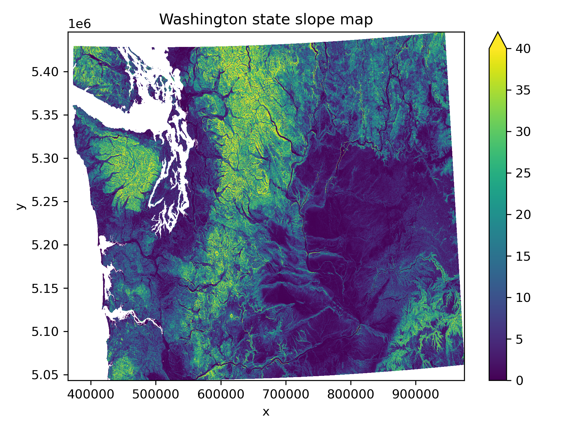
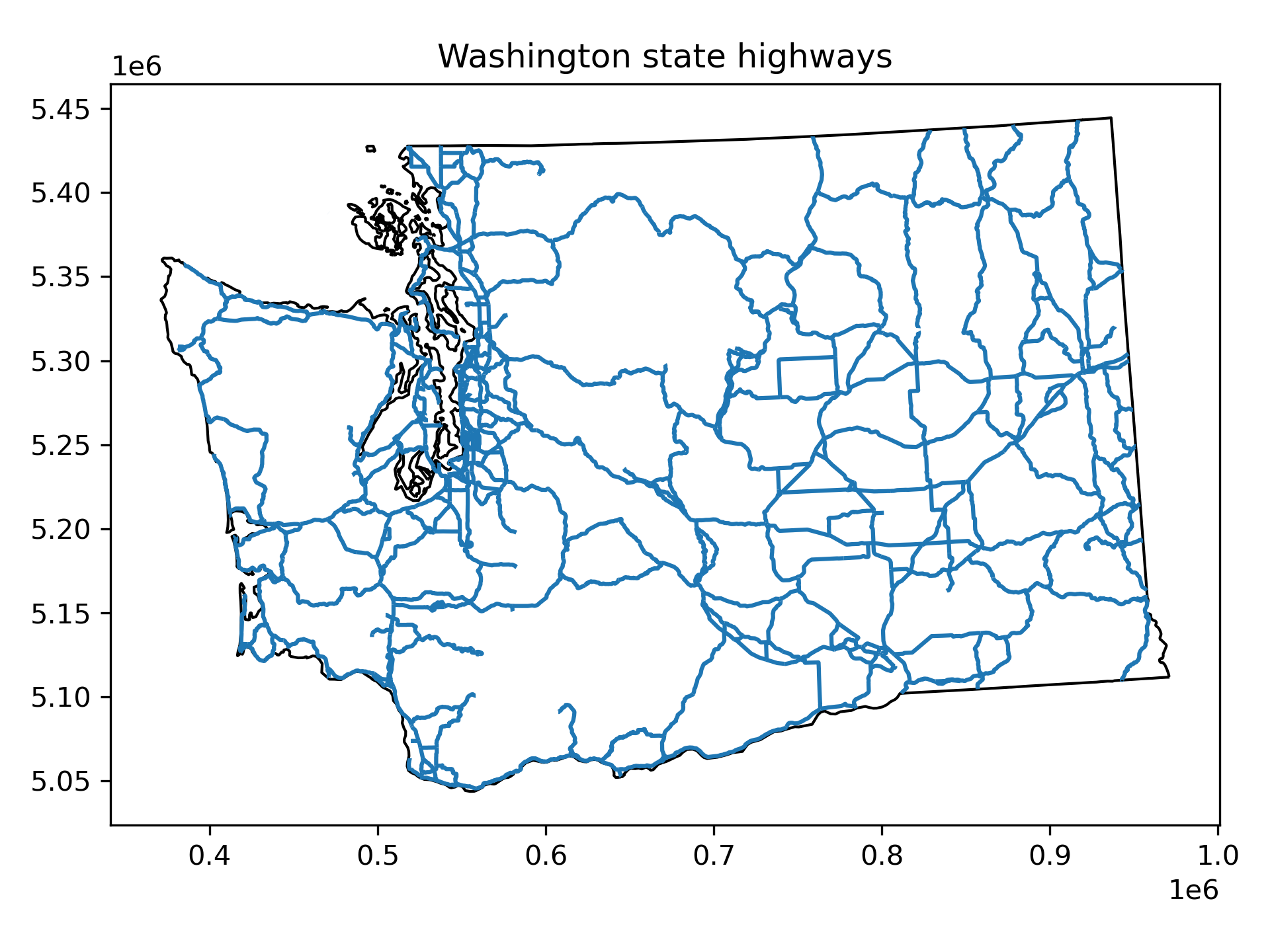
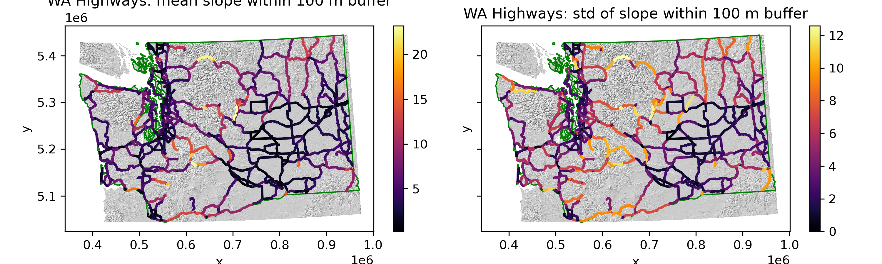
We’d like to answer the question: Which sections of WA highways are surrounded by the steepest slopes?
Requires sampling a derived DEM product (slope) around Polyline objects (highways)
This is important for geohazards (rockfall, avalanches)
You can probably make an informed guess here based on knowledge of the terrain and WA highway network
Note that in practice, you would want to higher resolution DEM with higher accuracy (e.g., DTM from airborne lidar), but same concept/method applies
Compute surface slope and plot#
Easy to use
gdaldemcommand line utility here (like hillshade generation above) to create a new tif file with slope valuesCan also compute slope directly from our DEM array using
np.gradient
slope_fn = os.path.splitext(proj_fn)[0]+'_slope.tif'
# STUDENT CODE HERE
# STUDENT CODE HERE
<xarray.DataArray (y: 5851, x: 8877)> Size: 208MB
[51939327 values with dtype=float32]
Coordinates:
    band         int64 8B 1
  * x            (x) float64 71kB 3.647e+05 3.648e+05 ... 9.748e+05 9.749e+05
  * y            (y) float64 47kB 5.446e+06 5.446e+06 ... 5.043e+06 5.043e+06
    spatial_ref  int64 8B 0
Attributes:
    AREA_OR_POINT:  Area
    scale_factor:   1.0
add_offset: 0.0# STUDENT CODE HERE
Prepare highway data#
We’ll use some polyline data from Washington State Department of Transportation (WSDOT) here
https://www.wsdot.wa.gov/mapsdata/geodatacatalog/maps/NOSCALE/DOT_TDO/LRS/sr500kjpg.htm
from datetime import datetime
year = datetime.now().year - 2
#year = 2021

#Link to WA DOT highway data (requires updating each year)
#wa_dot_highway_url = 'https://data.wsdot.wa.gov/geospatial/DOT_TDO/LRS/Historic/500kLRS_2020.zip'
wa_dot_highway_url = f'https://data.wsdot.wa.gov/geospatial/DOT_TDO/LRS/500kLRS_{year}.zip'
#Relative path of the shapefile within the zip archive
wa_dot_highway_shp_fn = f'500k/sr500klines_{year}1231.shp'

#Open zip file and contained shapefile on-the-fly with GeoPandas
highways_gdf = gpd.read_file(f'zip+{wa_dot_highway_url}!{wa_dot_highway_shp_fn}')
highways_gdf = highways_gdf.to_crs(dst_crs)
highways_gdf
| BARM | EARM | REGION | DISPLAY | RT_TYPEA | RT_TYPEB | LRS_Date | RouteID | StateRoute | RelRouteTy | RelRouteQu | SHAPE_STLe | geometry | |
|---|---|---|---|---|---|---|---|---|---|---|---|---|---|
| 0 | 212.81 | 213.46 | EA | 2 | US | 2 | 20231231 | 002 | 002 | None | None | 3413.387059 | LINESTRING (820555.58 5298852.974, 820619.146 ... |
| 1 | 213.46 | 242.68 | EA | 2 | US | 2 | 20231231 | 002 | 002 | None | None | 154217.182705 | LINESTRING (821529.627 5298486.191, 822158.751... |
| 2 | 242.68 | 243.47 | EA | 2 | US | 2 | 20231231 | 002 | 002 | None | None | 4116.114242 | LINESTRING (863590.057 5289216.121, 864246.265... |
| 3 | 243.47 | 253.01 | EA | 2 | US | 2 | 20231231 | 002 | 002 | None | None | 50376.876336 | LINESTRING (864829.94 5289365.616, 865088.408 ... |
| 4 | 253.01 | 255.89 | EA | 2 | US | 2 | 20231231 | 002 | 002 | None | None | 15290.597916 | LINESTRING (880029.098 5291008.477, 881836.927... |
| ... | ... | ... | ... | ... | ... | ... | ... | ... | ... | ... | ... | ... | ... |
| 1035 | 0.48 | 0.51 | SC | 970 | SR | 0 | 20231231 | 970 | 970 | None | None | 467.956867 | LINESTRING (659291.702 5228115.833, 659429.812... |
| 1036 | 0.51 | 0.60 | SC | 970 | SR | 0 | 20231231 | 970 | 970 | None | None | 646.207071 | LINESTRING (659429.812 5228080.232, 659612.641... |
| 1037 | 0.60 | 2.69 | SC | 970 | SR | 0 | 20231231 | 970 | 970 | None | None | 9945.506285 | LINESTRING (659612.641 5228006.991, 660348.756... |
| 1038 | 2.69 | 10.31 | SC | 970 | SR | 0 | 20231231 | 970 | 970 | None | None | 40612.531248 | LINESTRING (662410.766 5226841.516, 662759.34 ... |
| 1039 | 0.00 | 15.02 | NC | 971 | SR | 0 | 20231231 | 971 | 971 | None | None | 76589.725431 | LINESTRING (711509.694 5294629.359, 711220.395... |
1040 rows × 13 columns
Plot the highway data#
# STUDENT CODE HERE
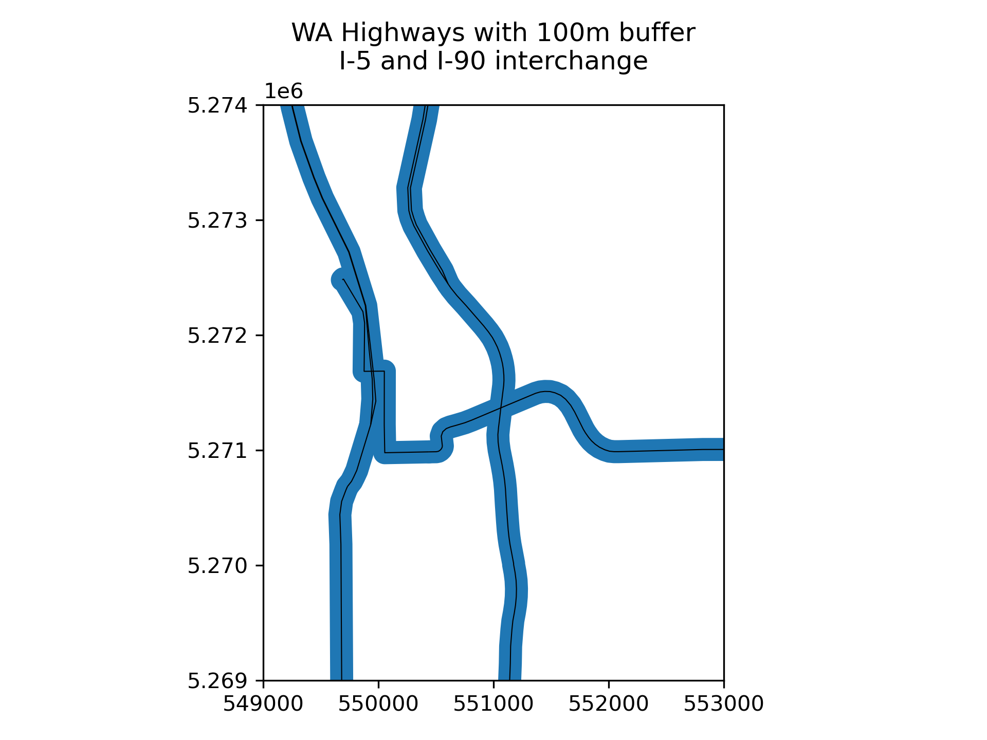
Compute polygons for a 100 m buffer around the polylines. Create a sample plot around the I-5 and I-90 interchange with the original and buffered lines.#
Remember that the output of
bufferis a GeoSeries of Polygons - want to create a new GeoDataFrame and use this as thegeometryTo select the I-5 and I-90 area you can use these limits:
ax.set_ylim(5.269E6, 5.274E6)ax.set_xlim(5.49E5, 5.53E5)
# STUDENT CODE HERE
| BARM | EARM | REGION | DISPLAY | RT_TYPEA | RT_TYPEB | LRS_Date | RouteID | StateRoute | RelRouteTy | RelRouteQu | SHAPE_STLe | geometry | |
|---|---|---|---|---|---|---|---|---|---|---|---|---|---|
| 0 | 212.81 | 213.46 | EA | 2 | US | 2 | 20231231 | 002 | 002 | None | None | 3413.387059 | POLYGON ((820647.736 5298929.835, 820656.174 5... |
| 1 | 213.46 | 242.68 | EA | 2 | US | 2 | 20231231 | 002 | 002 | None | None | 154217.182705 | POLYGON ((822167.307 5298420.143, 822657.594 5... |
| 2 | 242.68 | 243.47 | EA | 2 | US | 2 | 20231231 | 002 | 002 | None | None | 4116.114242 | POLYGON ((864239.532 5289359.444, 864518.698 5... |
| 3 | 243.47 | 253.01 | EA | 2 | US | 2 | 20231231 | 002 | 002 | None | None | 50376.876336 | POLYGON ((865036.585 5289607.756, 865043.098 5... |
| 4 | 253.01 | 255.89 | EA | 2 | US | 2 | 20231231 | 002 | 002 | None | None | 15290.597916 | POLYGON ((881799.822 5291819.793, 882495.798 5... |
| ... | ... | ... | ... | ... | ... | ... | ... | ... | ... | ... | ... | ... | ... |
| 1035 | 0.48 | 0.51 | SC | 970 | SR | 0 | 20231231 | 970 | 970 | None | None | 467.956867 | POLYGON ((659454.773 5228177.067, 659464.145 5... |
| 1036 | 0.51 | 0.60 | SC | 970 | SR | 0 | 20231231 | 970 | 970 | None | None | 646.207071 | POLYGON ((659649.828 5228099.819, 659658.748 5... |
| 1037 | 0.60 | 2.69 | SC | 970 | SR | 0 | 20231231 | 970 | 970 | None | None | 9945.506285 | POLYGON ((660385.941 5227804.949, 660387.648 5... |
| 1038 | 2.69 | 10.31 | SC | 970 | SR | 0 | 20231231 | 970 | 970 | None | None | 40612.531248 | POLYGON ((662737.254 5226952.755, 663204.724 5... |
| 1039 | 0.00 | 15.02 | NC | 971 | SR | 0 | 20231231 | 971 | 971 | None | None | 76589.725431 | POLYGON ((709446.871 5305866.855, 709539.519 5... |
1040 rows × 13 columns
# STUDENT CODE HERE
Now use rasterstats.zonal_stats to compute and plot slope statistics within those polygons#
See the
rasterstatsdocumentation: https://pythonhosted.org/rasterstats/manual.html#zonal-statisticsThe docs example uses a shapefile on disk and raster on disk, but we already have our features and raster loaded in memory!
Can pass in the GeoDataFrame containing buffered Polygon features instead of a filename
Can pass in the slope NumPy array instead of the xarray dataarray (remember to use
.valuesto access the underlying numpy array), but need to provide the appropriatetransformto theaffinekeywordShould also pass the appropriate rasterio dataset
nodatavalue
Compute stats and add the following columns to the
highways_gdfgeodataframe for each highway segment:mean slope
std of slope (a roughness metric)
Create some plots to visualize
If you’re plotting the GeoDataFrame containing the original LINESTRING geometry objects, choose an appropriate
linewidth
# STUDENT CODE HERE
# STUDENT CODE HERE
# STUDENT CODE HERE
# STUDENT CODE HERE
Sort the highway sections by either their respective slope mean or standard deviation with the highest values at the top. Plot the sections of highway with the 5 highest of these values.#
# STUDENT CODE HERE
# STUDENT CODE HERE
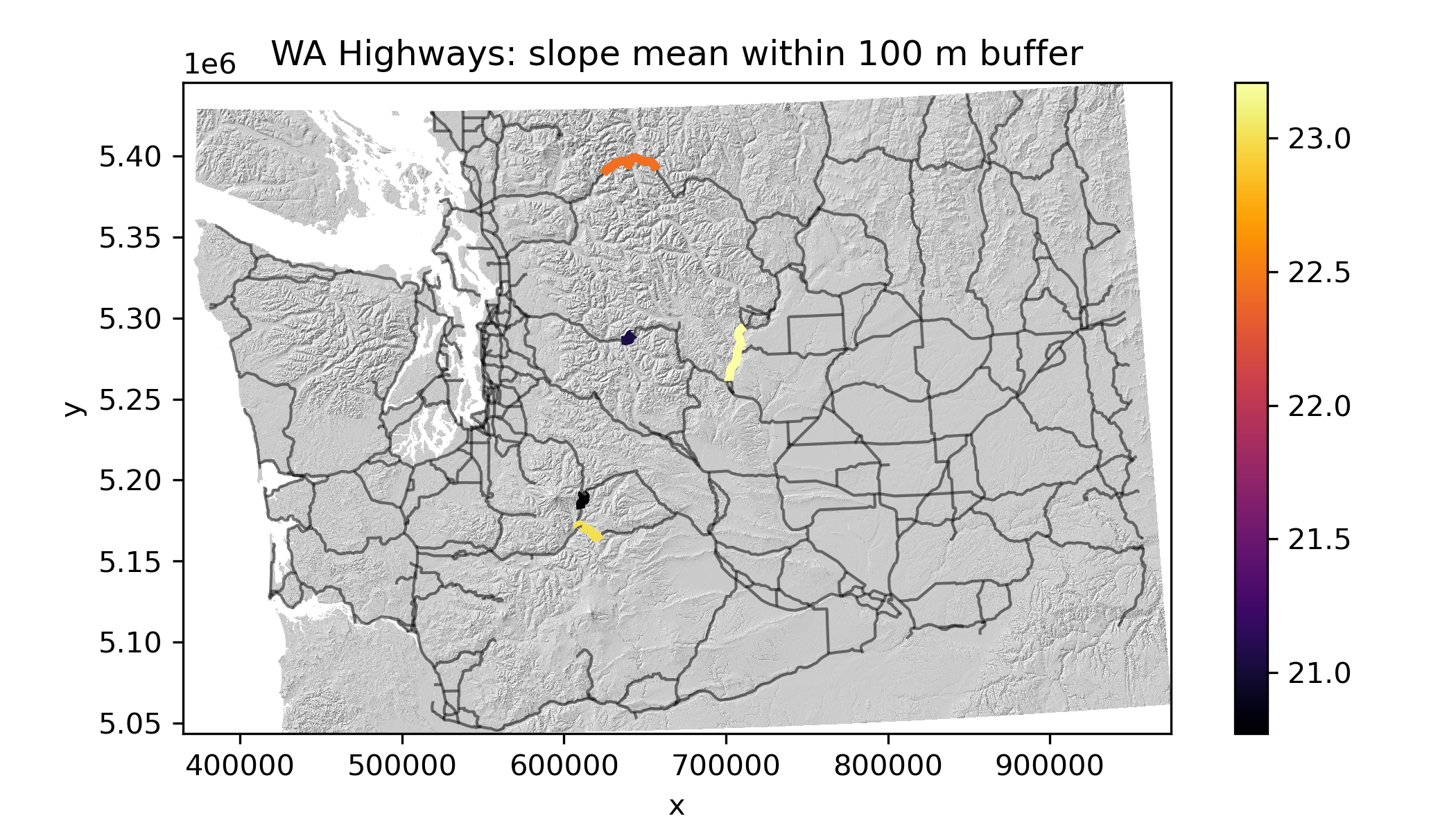
Written response: Which section of the highway might you close first during periods of extreme winter weather?#
STUDENT WRITTEN RESPONSE HERE
Submission#
Save the completed notebook (make sure to fully run the notebook and check all cell output is visible)
Use the
git add; git commit -m 'message'; git pushworkflow to push your work to the remote repositoryideally you’ve been using add / commit / push as you make progress on this notebook
Check the remote repository to check all of the files you want to submit have been pushed
Scroll through your jupyter notebook on your remote repository and make sure all output and plots are visible
When you have completed your last push, submit the url pointing to your Github repository to the corresponding Canvas assignment