Lab 09 assignment notebook 1 (20 pts)

Lab 09 assignment notebook 1 (20 pts)#

Notebook 1 of 2

UW Geospatial Data Analysis
CEE467/CEWA567
David Shean, Eric Gagliano, Quinn Brencher

Introduction#

Objectives#

Get experience pulling in data from STAC catalogs
Get experience designing well-crafted, well-documented functions and classes
Explore Python script, module and package creation
Explore coseismic landslide detection using Sentinel-2 NDVI time series
Get exposure to Dask and continue exploring our core geospatial packages
Get exposure to some basic computer vision approaches for raster analysis

Instructions#

For each question or task below, write some code in the empty cell and execute to preserve your output
If you are in the graduate section of the class, please complete the challenge questions
Work together, consult resources we’ve discussed, post on Slack!
Follow the submission instructions at the end of the lab!

Background#

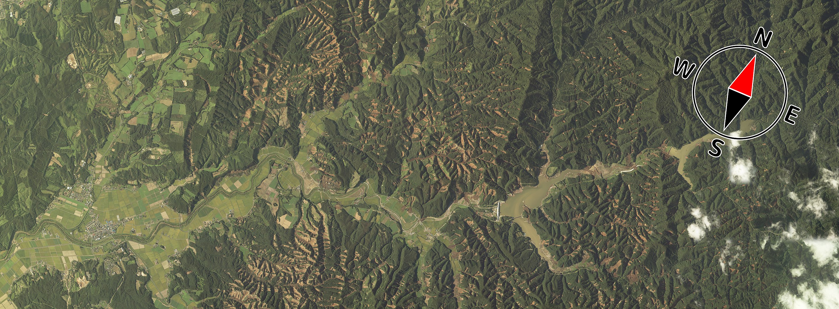
In this lab, we’re going to design a Python workflow that creates inventories of earthquake-triggered (coseismic) landslides. Our work will culminate in a script that takes an earthquake date and a bounding box and produces an inventory of landslides that have occured following the earthquake using change in NDVI. Coseismic landslides can compound the damage caused by earthquakes and are a major concern in the Pacific Northwest. After an earthquake occurs, identifying the location of landslides using remote sensing data can help with disaster response. To develop our landslide inventory workflow, we’ll use the 2018 Hokkaido Eastern Iburi earthquake in Japan, which caused ~5,600 landslides. This earthquake and the ensuing landslides were responsible for $3.32 billion in damage, 41 deaths, and 691 injuries.

../../_images/2db7b1cd-1ee1-4830-9def-07d85096f5b1-Quake008.webp

../../_images/2880px-Ground_surface_in_northern_Atsuma_Town_after_2018_earthquake.jpg

import pystac_client
import planetary_computer
import xarray as xr
import rasterio as rio
import rioxarray
import geopandas as gpd
import odc.stac
import matplotlib.pyplot as plt
import pandas as pd
import numpy as np
from scipy.optimize import curve_fit
import os
import rasterstats
from rioxarray import merge
import scipy.ndimage as ndimage
from skimage.segmentation import watershed
from skimage.feature import peak_local_max
from skimage.measure import label
from shapely.geometry import shape
from rasterio.features import shapes, rasterize
import xyzservices.providers as xyz

Part 1: Loading data (4 pts)#

To detect landslides, we’re going to use Sentinel-2 imagery to create an NDVI time series. Where there’s a substantial decrease in NDVI, we can infer that a landslide likely occured. Ideally, we would simply compare NDVI before and after the earthquake, and wherever NDVI decreased by a certain amount, we would classify that pixel as a landslide. The trouble is that NDVI changes seasonally as plants adjust to winter, crops are harvested, etc. Any changes in NDVI caused by landslides will be superimposed on this seasonal change, and it may be difficult to tell if a drop in NDVI is caused by a normal seasonal change or a landslide.

To address this issue, rather than comparing NDVI immediately before and after the earthquake, we’ll try to measure how different NDVI is from normal NDVI during a given season, before and after the earthquake. In other words, we’re going to compute the NDVI anomaly (difference from median NDVI in a given season). To do this, we first need to compute median NDVI for each season prior to the earthquake.

1.1 Seasonal NDVI#

Query the Planetary Computer STAC catalog to find Sentinel-2 Level 2A data prior to the earthquake for our area of interest.#

Print the number of items returned.

use query={"eo:cloud_cover": {"lt": 80}} in your search to only include scenes with < 80% cloud cover.
As a start date for your search time period, you can use '2015-06-27', which is the beginning of the Sentinel-2 Level 2A data archive
To get an end date for your search time period, use the following function to find the day before the earthquake.

def calculate_date_before(date_str, days_padding=1):
    date = pd.Timestamp(date_str)  # Convert string to pandas Timestamp
    date_before = date - pd.DateOffset(days=days_padding)
    return date_before.strftime("%Y-%m-%d")

end_date = calculate_date_before(earthquake_date)

# STUDENT CODE HERE

Returned 62 Items

Use `odc-stac` to load these items into an Xarray dataset called `pre_earthquake_s2_ds`.#

Load only the Red, NIR, and Scene Classification Map (SCL) bands
Use chunks={"x": 256, "y": 256}
Use groupby='solar_day'
Load only the data within our bbox

Do not do .compute() yet!

# STUDENT CODE HERE

pre_earthquake_s2_ds

<xarray.Dataset> Size: 336MB
Dimensions:      (y: 565, x: 826, time: 60)
Coordinates:
  * y            (y) float64 5kB 4.734e+06 4.734e+06 ... 4.728e+06 4.728e+06
  * x            (x) float64 7kB 5.737e+05 5.737e+05 ... 5.819e+05 5.819e+05
    spatial_ref  int32 4B 32654
  * time         (time) datetime64[ns] 480B 2015-12-25T01:30:52.029000 ... 20...
Data variables:
    B04          (time, y, x) float32 112MB dask.array<chunksize=(1, 256, 256), meta=np.ndarray>
    B08          (time, y, x) float32 112MB dask.array<chunksize=(1, 256, 256), meta=np.ndarray>
    SCL          (time, y, x) float32 112MB dask.array<chunksize=(1, 256, 256), meta=np.ndarray>

Great! Now we’re going to:

Add a new band for NDVI
Mask unreliable pixels
Drop the variables we no longer need

We have done this for you.

# calculate NDVI
pre_earthquake_s2_ds['NDVI'] = (pre_earthquake_s2_ds['B08'] - pre_earthquake_s2_ds['B04'])/(pre_earthquake_s2_ds['B08'] + pre_earthquake_s2_ds['B04'])

# mask unreliable pixels
bad_scl = [0, 1, 8, 9]
pre_earthquake_s2_ds['NDVI'] = pre_earthquake_s2_ds['NDVI'].where(~pre_earthquake_s2_ds['SCL'].isin(bad_scl))

# drop unnneeded data variables 
pre_earthquake_s2_ds = pre_earthquake_s2_ds.drop_vars(['B04', 'B08', 'SCL'])

Plot median NDVI for each month#

# STUDENT CODE HERE

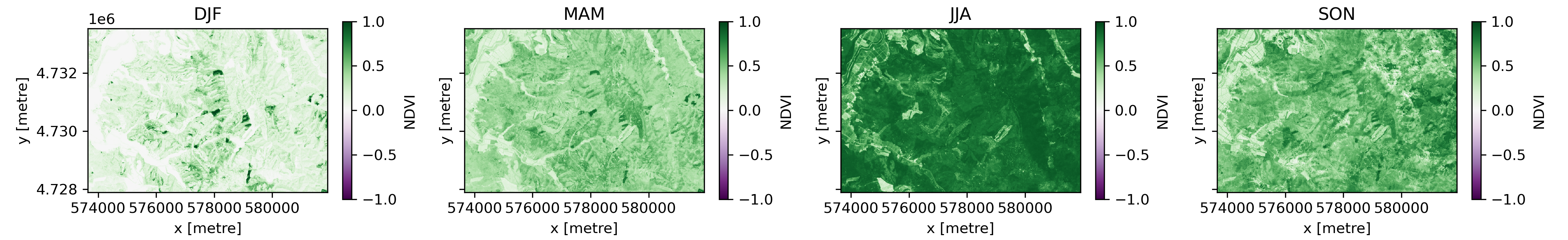
Written Response: Describe the seasonal evolution of NDVI at this location and speculate about what might cause it.#

STUDENT WRITTEN RESPONSE HERE

Excellent! Now we have our baseline seasonal NDVI that we can use to calculate the NDVI anomaly.

1.2 NDVI time series#

Now we need to create a Sentinel-2 NDVI time series that spans the period before and after the eartquake. Use the calculate_date_range function below to find the dates three months before and three months after the earthquake date (which we stored in a variable in Part 0).

def calculate_date_range(date_str, months_padding=3):
    date = pd.Timestamp(date_str)  # Convert string to pandas Timestamp
    start_date = date - pd.DateOffset(months=months_padding)
    end_date = date + pd.DateOffset(months=months_padding)
    return start_date.strftime("%Y-%m-%d"), end_date.strftime("%Y-%m-%d")

date_range = calculate_date_range(earthquake_date)

Query the Planetary Computer STAC catalog for Sentinel-2 images within our date range for our area of interest#

Again, print the number of items returned.

this time, use query={"eo:cloud_cover": {"lt": 50}}

# STUDENT CODE HERE

Returned 10 Items

Use `odc-stac` to load the data into an Xarray dataset called `s2_ds`#

Again,

Load only the Red, NIR, and Scene Classification Map (SCL) bands
Use chunks={"x": 256, "y": 256}
Use groupby='solar_day'
Load only the data within our bbox

Do not do .compute() yet!

# STUDENT CODE HERE

s2_ds

<xarray.Dataset> Size: 56MB
Dimensions:      (y: 565, x: 826, time: 10)
Coordinates:
  * y            (y) float64 5kB 4.734e+06 4.734e+06 ... 4.728e+06 4.728e+06
  * x            (x) float64 7kB 5.737e+05 5.737e+05 ... 5.819e+05 5.819e+05
    spatial_ref  int32 4B 32654
  * time         (time) datetime64[ns] 80B 2018-06-07T01:26:49.024000 ... 201...
Data variables:
    B04          (time, y, x) float32 19MB dask.array<chunksize=(1, 256, 256), meta=np.ndarray>
    B08          (time, y, x) float32 19MB dask.array<chunksize=(1, 256, 256), meta=np.ndarray>
    SCL          (time, y, x) float32 19MB dask.array<chunksize=(1, 256, 256), meta=np.ndarray>

As above, we have done the following for you:

Add a new band for NDVI
Mask unreliable pixels
Drop the variables we no longer need

# calculate NDVI
s2_ds['NDVI'] = (s2_ds['B08'] - s2_ds['B04'])/(s2_ds['B08'] + s2_ds['B04'])

# mask unreliable pixels
cloud_nodata_values = [0, 1, 8, 9]
s2_ds['NDVI'] = s2_ds['NDVI'].where(~s2_ds['SCL'].isin(cloud_nodata_values))

# drop unnneeded data variables 
s2_ds = s2_ds.drop_vars(['B04', 'B08', 'SCL'])

Ok, now for each NDVI raster in our time series, let’s calculate the NDVI anomaly. We’ll do this by subtracting the median monthly NDVI from each NDVI raster and creating a new data variable called 'NDVI_anomaly'. Next, we’ll do .compute() to trigger the computations and load the Dataset into memory. We have done this for you.

# extract month index from the time dimension of the time series dataset
s2_ds = s2_ds.assign_coords(season=s2_ds['time'].dt.season)

# calcualate the ndvi anomaly by subtracting the median monthly NDVI for the appropriate month
s2_ds['NDVI_anomaly'] = s2_ds['NDVI'] - seasonal_ds.sel(season=s2_ds['season'])['NDVI']

s2_ds = s2_ds.compute()

Now we’re ready to start looking for landslides!

Use the `s2_ds` Dataset to create a figure with the following 6 panels:#

Median NDVI before the earthquake
Median NDVI after the earthquake
Difference in median NDVI before vs after the earthquake
Median NDVI anomaly before the earthquake
Median NDVI anomaly after the earthquake
Difference in median NDVI anomaly before vs after the earthquake

# STUDENT CODE HERE

# STUDENT CODE HERE

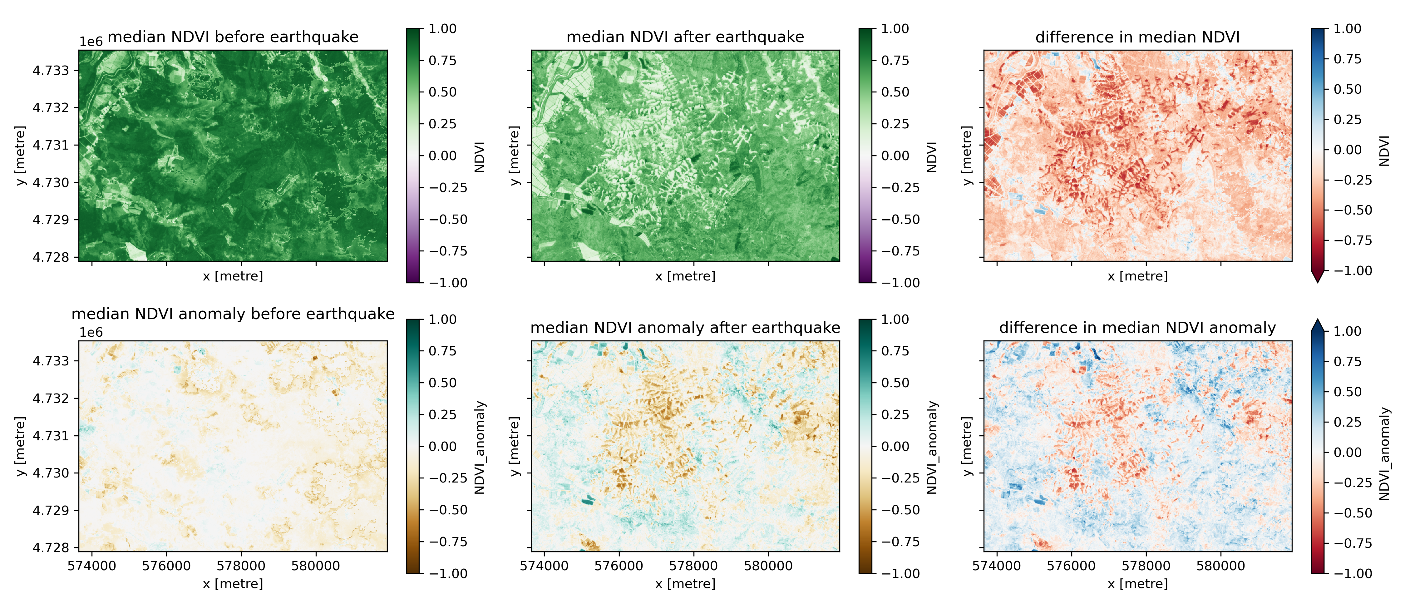
Written Response: Take a moment to consider these plots.#

Describe NDVI and NDVI anomaly change you beleive to be caused by landslides
Describe NDVI and NDVI anomaly change you beleive is not caused by landslides
Describe two other interesting things that you notice that may be relevant for this analysis. (Hint: take a look at the agricultural fields along the river in the top left corner of these plots).

STUDENT WRITTEN RESPONSE HERE

1.3 Copernicus 30m DEM#

Bring in a DEM for our area of interest.#

Query the Planetary Computer STAC catalog for the Copernicus 30m DEM tiles that overlap our area of interest and print how many items were returned. https://planetarycomputer.microsoft.com/dataset/cop-dem-glo-30

# STUDENT CODE HERE

Returned 2 Items

Great. Now use the code below to merge these tiles into a single Xarray DataArray, clip to the area of interest, and reproject to the same CRS as the Sentinel-1 images (the local UTM zone). We’ll pad the area of interest slightly to avoid issues at the edge of the DEM.

data = []
for item in items:
    dem_path = planetary_computer.sign(item.assets['data']).href
    data.append(rioxarray.open_rasterio(dem_path))
cop30_da = merge.merge_arrays(data)  
cop30_da = cop30_da.rio.write_nodata(0)

padding = 0.02 # degrees
padded_bbox = (bbox[0]-padding, bbox[1]-padding, bbox[2]+padding, bbox[3]+padding)

# clip to aoi
cop30_da = cop30_da.rio.clip_box(*padded_bbox,crs="EPSG:4326").squeeze()

# reproject to Sentinel-2 crs (UTM zone)
cop30_da = cop30_da.rio.reproject(s2_ds.rio.crs)

Part 2: Fitting a step function, landslide classification, generating a landslide inventory (3 pts)#

In this section, most of the code is written for you. There are a few spots where we ask for a small contribution or a written response. Nonetheless, please go through this code carefully so you understand what it does, as we’ll be using it later!

2.1 Fitting a step function#

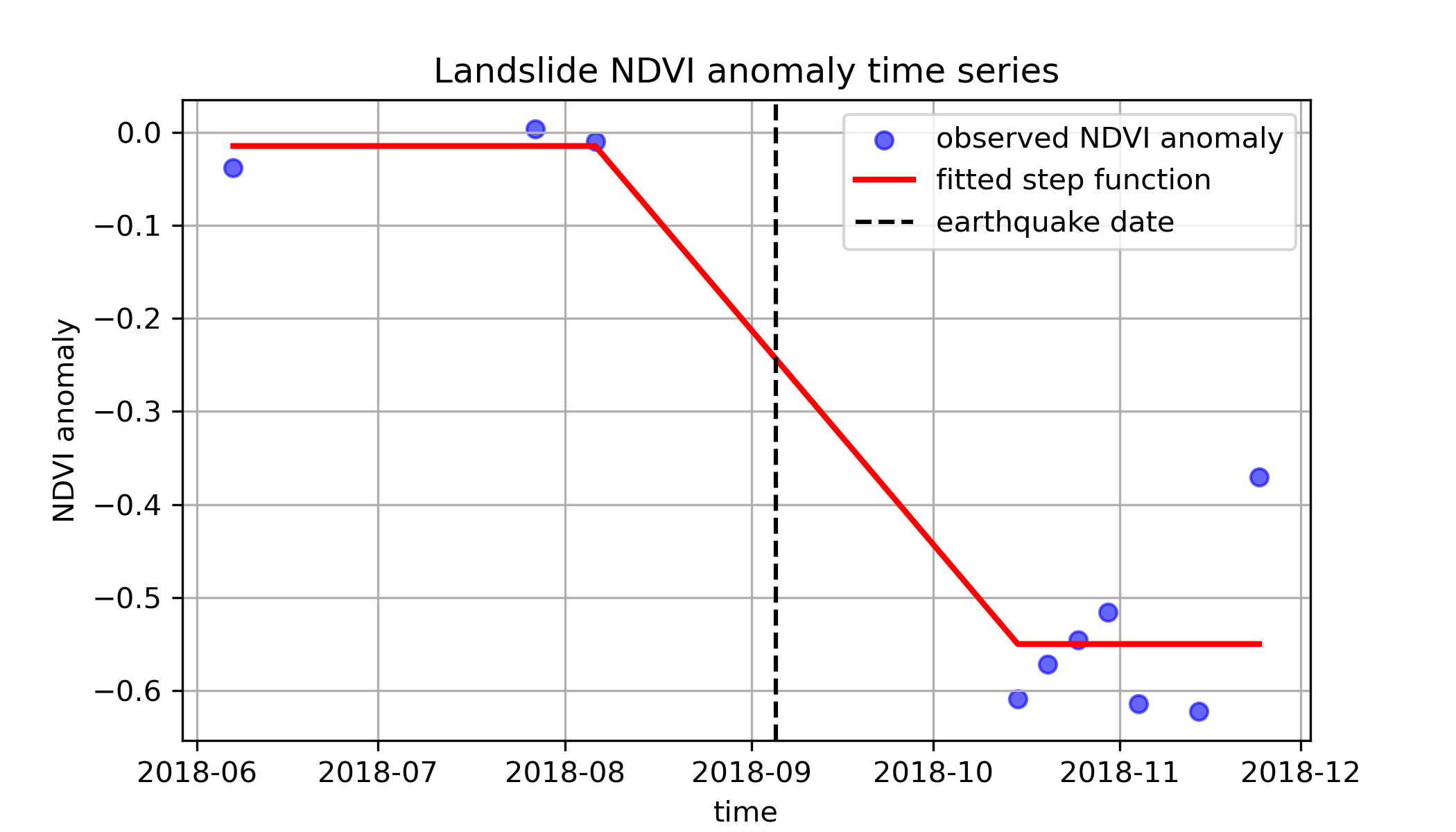
By computing the NDVI anomaly, we removed some of the normal variability in NDVI over time. We can potentially isolate the NDVI change cause by landslides further by fitting a step function to our NDVI time series. Let’s first take a look at the NDVI time series for a landslide pixel.

landslide_pixel = (573912.1,4732589.4)

# select time series for pixel
landslide_pixel_ndvi_anomaly = s2_ds.sel(x=landslide_pixel[0], y=landslide_pixel[1], method='nearest').NDVI_anomaly.values
time_values = s2_ds.time.values.astype(float) # convert to numeric for function fitting

f, ax = plt.subplots(1, 2, figsize=(10, 3))
ndvi_anomaly_difference.isel(x=slice(0,150), y=slice(0,150)).plot(ax=ax[0], vmin=-1, vmax=1, cmap='RdBu')
ax[0].scatter(landslide_pixel[0], landslide_pixel[1], c='k', label='landslide pixel')
ax[0].set_title('')
ax[1].scatter(s2_ds.time, landslide_pixel_ndvi_anomaly, c='k')
ax[1].axvline(pd.Timestamp(earthquake_date), color="black", linestyle="--", label="earthquake date")
ax[0].legend()
ax[1].legend()
ax[0].set_aspect('equal')
plt.tight_layout()
f.savefig('imgs/single_pixel_ts.png', dpi=300)

There’s a clear step in this time series. By fitting a step function to the time series, we can estimate the baseline NDVI anomaly, the NDVI anomaly change, and the time the step occurs.

def step_function(t, a, b, t0, k=10):
    return a + b / (1 + np.exp(-k * (t - t0)))  

# initial guesses: baseline NDVI anomaly, rough estimate NDVI anomaly change, and earthquake date
initial_guess = [0, -0.2, np.datetime64(earthquake_date).astype("datetime64[ns]").astype(float)]

params, _ = curve_fit(step_function, time_values, landslide_pixel_ndvi_anomaly, p0=initial_guess)

a_fit, b_fit, t0_fit = params

# Generate fitted values using the best-fit parameters
fitted_values = step_function(time_values, a_fit, b_fit, t0_fit)

print(f'estimated initial NDVI anomaly: {a_fit},\nestimated NDVI anomaly step: {b_fit},\nestimated step date: {np.datetime64(int(t0_fit), "ns")}')

estimated initial NDVI anomaly: -0.014894704023997023,
estimated NDVI anomaly step: -0.5350755451400695,
estimated step date: 2018-09-05T00:00:00.000000000

f, ax = plt.subplots(figsize=(7, 4))
ax.scatter(s2_ds.time, landslide_pixel_ndvi_anomaly, color="blue", label="observed NDVI anomaly", alpha=0.6)
# Plot fitted step function
ax.plot(s2_ds.time, fitted_values, color="red", label="fitted step function", linewidth=2)
# plot earthquake date
ax.axvline(pd.Timestamp(earthquake_date), color="black", linestyle="--", label="earthquake date")

plt.xlabel("time")
plt.ylabel("NDVI anomaly")
plt.title("Landslide NDVI anomaly time series")
plt.legend()
plt.grid()

f.savefig('imgs/step_function.png', dpi=300)

Ok, now let’s fit a step function to every pixel in our Dataset! We’re going to have to include some additional code to handle NaN values. We have created a function for this below.

def fit_step_function(observed_values, time_values, date_of_interest):
    """Fit step function to a single pixel time series."""
    # mask nodata values 
    mask = ~np.isnan(observed_values)
    
    if np.sum(mask) < 5:  # skip if not enough valid points
        return np.nan, np.nan, np.nan
    
    try:
        # convert valid values
        t_valid = time_values[mask].astype(float)
        observed_valid = observed_values[mask]

        # initial guesses: baseline observed value, rough estimate observed value change, and date of interest
        p0 = [0, -0.2, np.datetime64(date_of_interest).astype("datetime64[ns]").astype(float)]
        
        # fit the step function
        params, _ = curve_fit(step_function, t_valid, observed_valid, p0=p0)

        return params[0], params[1], params[2]  # a (baseline), b (step size), t0 (change date)

    except RuntimeError:
        return np.nan, np.nan, np.nan  # return NaN if fitting fails

Now let’s actually apply our fitting function to every pixel. To do this, we’re going to use a ufunc. This will take a minute to run!

# convert time to numeric for fitting
time_numeric = s2_ds.time.values.astype(float)

# apply the function!
results = xr.apply_ufunc(
    fit_step_function, 
    s2_ds.NDVI_anomaly,  # NDVI values
    time_numeric,  # time values (passed separately)
    earthquake_date, # intial guess for step date
    input_core_dims=[["time"], ["time"], []],  # apply function along time axis
    output_core_dims=[[], [], []],  # three scalar outputs per pixel
    vectorize=True,  # allows working on multiple pixels at once
    dask="parallelized",  # uses Dask
    output_dtypes=[float, float, float],  # data types of outputs
)

# add the NDVI anomaly step size as new data variable in our time series dataset
s2_ds = s2_ds.assign(
    NDVI_anomaly_step=(["y", "x"], results[1].values),
)

Create a plot with three panels:#

Difference in median NDVI before vs after the earthquake
Difference in median NDVI anomaly before vs after the earthquake
The NDVI anomaly step from our fitted step function

# STUDENT CODE HERE

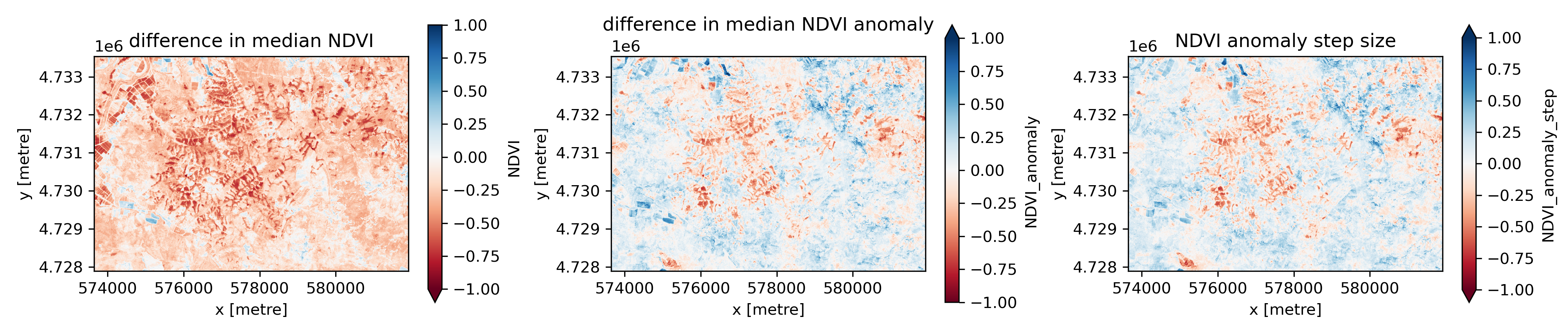
../../_images/ndvi_change_measurements.png

Written Response: Consider these plots.#

Which one of them looks like it will work best for identifying landslides using a threshold value in this case?
What do you think an appropriate threshold value might would be, for the one you think is most promising?
Under what circumstances would you expect each of the approaches to isolate the signal from landslides?

STUDENT WRITTEN RESPONSE HERE

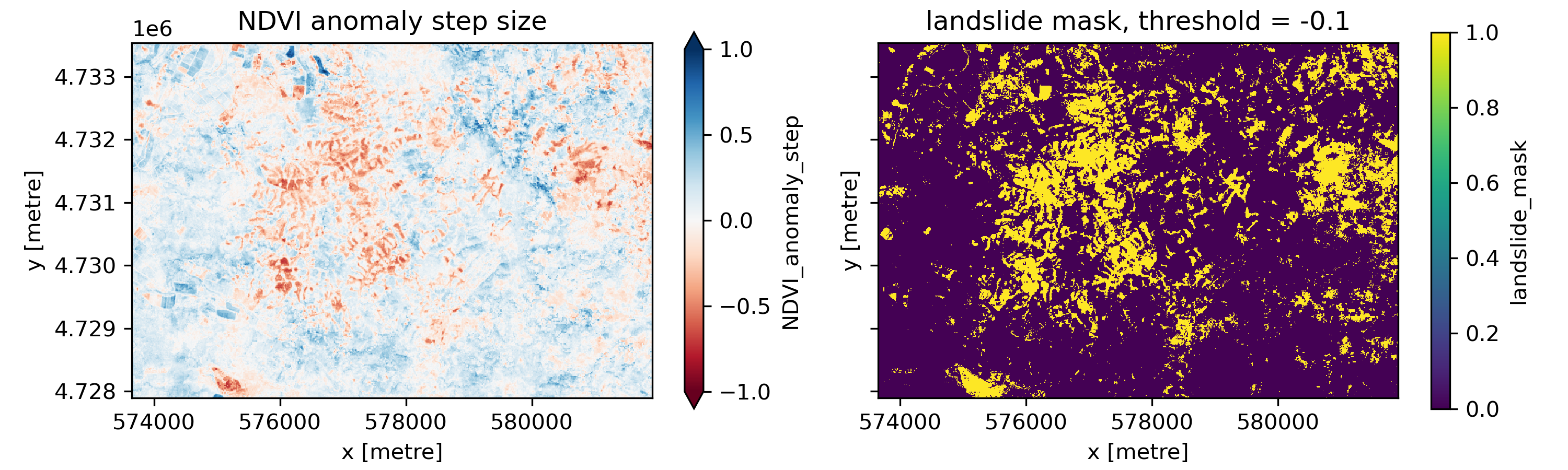
2.2 Classifying landslides#

Let’s use a simple threshold to classify which pixels are landslide pixels. You’re free to use the difference in NDVI before and after the earthquake, the difference in NDVI anomaly before and after the earthquake, or the NDVI anomaly step. Create a new data variable in our s2_ds Dataset called landslide_mask. This should be a boolean array with 1 for landslide pixels and 0 for non-landslide pixels.

# STUDENT CODE HERE

Create a plot that shows your mask next to the raster that it’s based on.#

You may want to use this plot to adjust your threshold.

# STUDENT CODE HERE

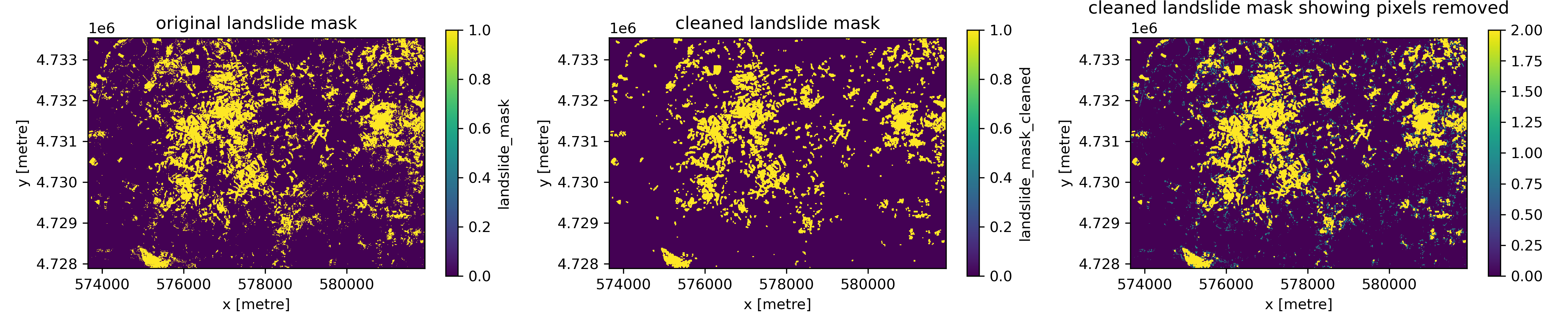
Notice that your landslide mask likely has lots of stray single pixels in it, which probably don’t correspond to landslides. We’ll clean this mask up using an erosion and dilation operation. In the erosion step, we pass a small 3 by 3 array over the landslide mask, so it’s centered on each pixel in the array. At each location, if all the pixels overlapping the 3 by 3 array are 1 (landslide), the center pixel in our landslide mask remains one. Otherwise, it’s set to 0. This has the effect of removing stray pixels that are incorrectly classified as landslides.

The dilation step does the opposite. The 3 by 3 array is passed over the landslide mask we just did the erosion operation on. If any pixel overlapping the 3 by 3 array has a value of 1, the center pixel is set to 1. Otherwise, it’s set to 0. This reverses the effect of the erosion for contiguous groups of pixels, but not for stray pixels that weren’t surrounded by other pixels classified as landslide. If you want to think more about these steps, check out the following blog post: https://medium.com/@sasasulakshi/opencv-morphological-dilation-and-erosion-fab65c29efb3

# define structuring element (3x3 cross or square)
structure = np.ones((3, 3), dtype=bool) 

# convert to NumPy array for processing
mask_np = s2_ds['landslide_mask'].values

# apply erosion followed by dilation (opening operation)
eroded = ndimage.binary_erosion(mask_np, structure=structure)
cleaned_mask = ndimage.binary_dilation(eroded, structure=structure)

# assign the cleaned mask back to the dataset
s2_ds = s2_ds.assign(landslide_mask_cleaned=(["y", "x"], cleaned_mask))

f, ax = plt.subplots(1, 3, figsize=(15, 3))
s2_ds['landslide_mask'].plot(ax=ax[0])
ax[0].set_aspect('equal')
ax[0].set_title('original landslide mask')
s2_ds['landslide_mask_cleaned'].plot(ax=ax[1])
ax[1].set_aspect('equal')
ax[1].set_title('cleaned landslide mask')
(s2_ds['landslide_mask_cleaned'].astype(int) + s2_ds['landslide_mask'].astype(int)).plot(ax=ax[2])
ax[2].set_aspect('equal')
ax[2].set_title('cleaned landslide mask showing pixels removed')
f.tight_layout()

f.savefig('imgs/erosion_dilation.png', dpi=300)

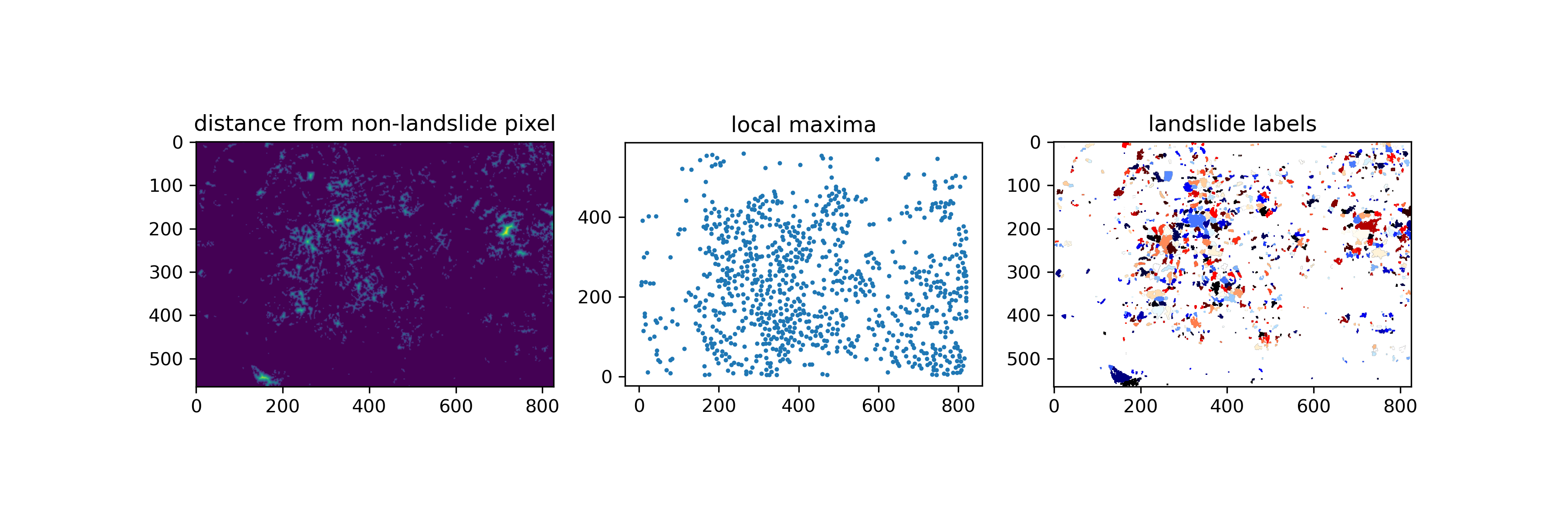
2.3 Segmenting landslides#

Now our landslide mask is a lot less noisy! But unfortunately, it looks like a lot of our landslides are grouped into big blobs, where individual landslides appear connected. How can we separate these connected areas into distinct landslides? Let’s use another image processing approach.

First, we’re going to use scipy.ndimage.distance_transform_edt() to calculate the distance between each landslide pixel and the nearest non-landslide pixel. We’ll save this as an array called distance. Next, we’re going to find the local maxima in our distance array using the skimage.feature.peak_local_max() function. We’ll pass min_distance=5 to ensure that our peaks are 5 pixels (50 m) apart. This is somewhat arbitrary, but ok for this simple example segmentation approach. Our local maxima are output as a list of [x, y] image coordinates rather than an image. So we need to create an empty array and fill in all of our local maxima locations with True. Next, we’ll use scipy.ndimage.label() on our local_maxi array to assign a different integer value (label) to each of our local maxima. Finally, we’re going to use the very cool skimage.segmentation.watershed() function. This function treats pixel values like topography, and floods topographic lows until basins attributed to different markers meet on watershed lines. In this case, we’ll use -distance as our topography–higher values will be closer to landslide boundaries, where lower values will be closer to landslide centers. Our local maxima will serve as the markers. This actually allows us to segment our different landslides!

# convert landslide mask to integer (1 = landslide, 0 = background)
landslide_mask = s2_ds.landslide_mask_cleaned.values.astype(int)

# compute distance from non-landslide pixel
distance = ndimage.distance_transform_edt(landslide_mask)

# get local maxima as coordinates
coordinates = peak_local_max(distance, labels=landslide_mask, min_distance=5)

# create an empty mask with the same shape as `distance`
local_maxi = np.zeros_like(distance, dtype=bool)

# set local maxima positions to True
local_maxi[tuple(coordinates.T)] = True  # Convert coordinates to indices

# give each local maxima a unique marker value
markers, _ = ndimage.label(local_maxi)

# apply watershed segmentation to separate landslides
labeled_landslides = watershed(-distance, markers, mask=landslide_mask)

# assign the split landslide IDs back to dataset
s2_ds = s2_ds.assign(landslide_id=(["y", "x"], labeled_landslides))

f, ax = plt.subplots(1, 3, figsize=(12, 4))
ax[0].imshow(distance)
ax[0].set_aspect('equal')
ax[0].set_title('distance from non-landslide pixel')
ax[1].scatter([xy_pair[1] for xy_pair in coordinates], [xy_pair[0] for xy_pair in coordinates], s=2)
ax[1].set_aspect('equal')
ax[1].set_title('local maxima')
ax[2].imshow(np.where(labeled_landslides > 0, labeled_landslides, np.nan), cmap='flag')
ax[2].set_aspect('equal')
ax[2].set_title('landslide labels', )
f.savefig('imgs/landslide_segmentation.png', dpi=300)

../../_images/landslide_segmentation.png

2.4 Polygonizing landslides and calculating zonal statistics#

Now that we have a different label (integer value) for each landslide, our next step is to turn our landslide labels from a raster into a vector dataset. We can do this using the rasterio.features.shapes() function, which will get the shapes and values of labelled regions in an array.

# initialize list for polygons and values
polygons = []
values = []

for geom, value in shapes(s2_ds.landslide_id.values, mask=s2_ds.landslide_id.values > 0, transform=s2_ds.rio.transform()):
    polygons.append(shape(geom))  # convert to Shapely polygon
    values.append(value)  # store landslide label

# create GeoDataFrame
landslides_gdf = gpd.GeoDataFrame({"landslide_id": values, "geometry": polygons}, crs=s2_ds.rio.crs)

To explore our brand new GeoDataFrame, use geopandas .explore() function with tiles=xyz.Esri.WorldImagery). When you’re done, comment this plot out to save space before submitting.

# landslides_gdf.explore(tiles=xyz.Esri.WorldImagery)

Written Response: Consider the landslide inventory.#

Where do you see false positives?
Where do you see false negatives?
How did our segmentation approach do to separate different landslides?

STUDENT RESPONSE HERE

Plot the landslide inventory on top of the DEM DataArray we pulled in in Part 1.#

Use the bounds of the landslide geodataframe as the bounds of the plot.

landslides_gdf.total_bounds

array([ 573670., 4727890.,  581910., 4733540.])

# STUDENT CODE HERE

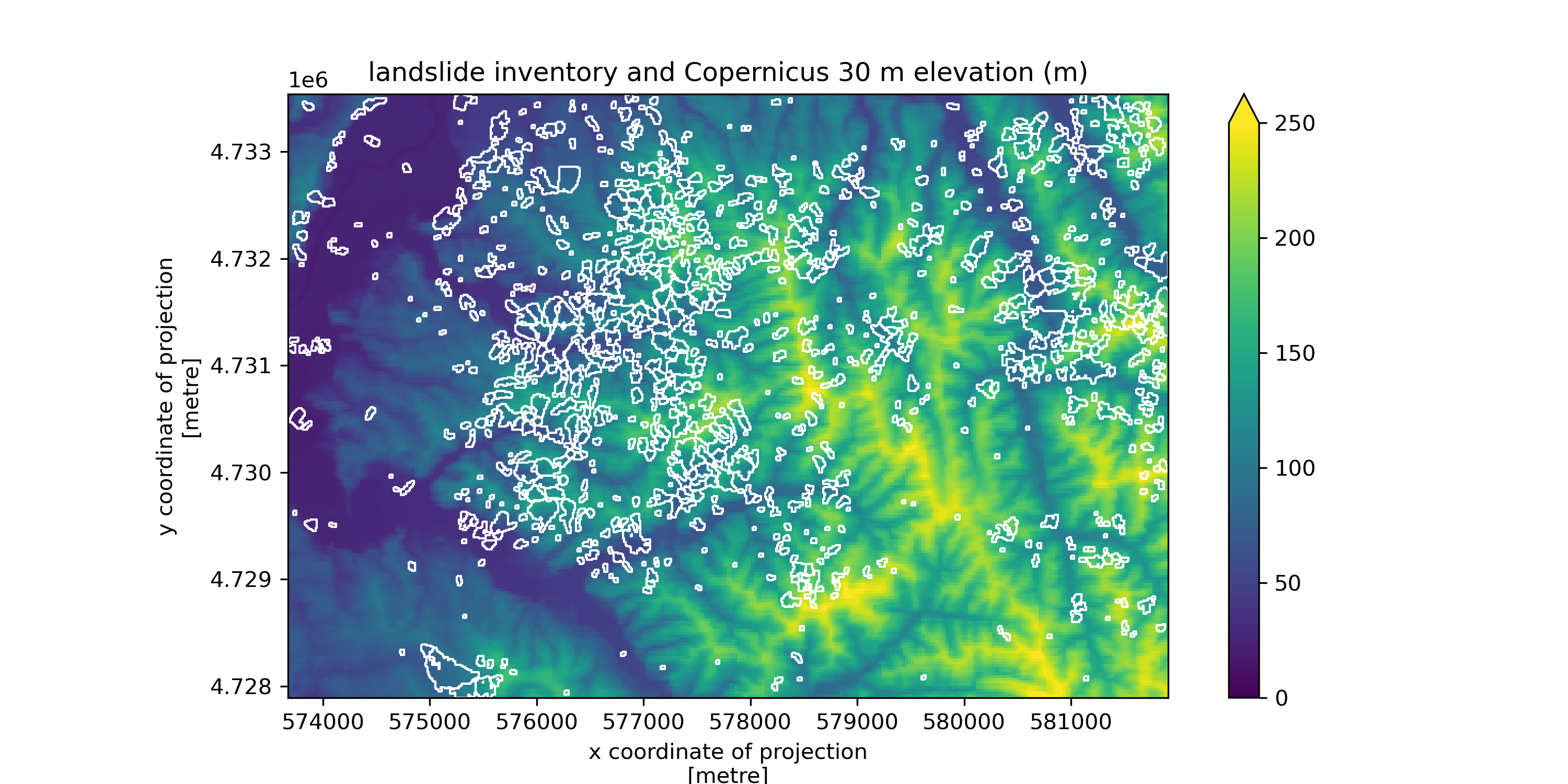
Now let’s calculate some statistics for our landslide inventory. For each landslide, we want to know total area, mean slope, and mean elevation. This means that we need to use our DEM data to make a new slope raster!

os.makedirs('data', exist_ok=True)

dem_fn = 'data/cop30.tif'
cop30_da.rio.to_raster(dem_fn)

slope_fn = 'data/cop30_slope.tif'
if not os.path.exists(slope_fn):
    !gdaldem slope $dem_fn $slope_fn 

slope_da = rioxarray.open_rasterio(slope_fn).squeeze()
slope_da = slope_da.where(slope_da >= 0)

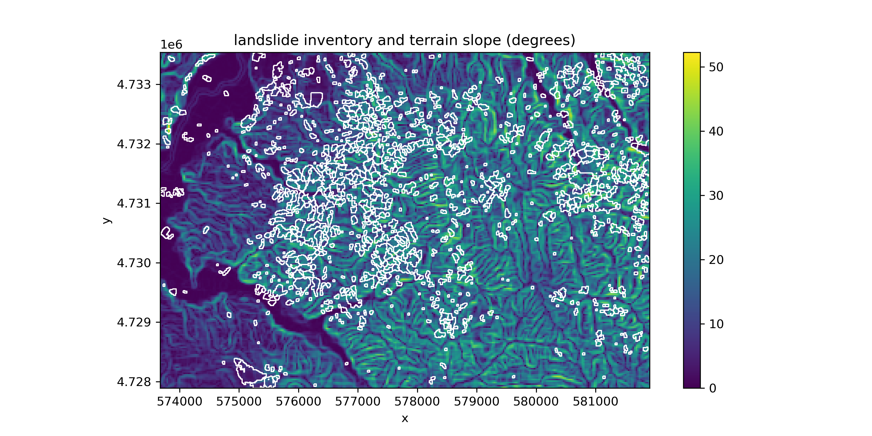
f, ax = plt.subplots(figsize=(10, 5))
slope_da.plot.imshow(ax=ax)
landslides_gdf.plot(ax=ax, facecolor='none', edgecolor='white', linewidth=1)
ax.set_xlim(landslides_gdf.total_bounds[0], landslides_gdf.total_bounds[2])
ax.set_ylim(landslides_gdf.total_bounds[1], landslides_gdf.total_bounds[3])
ax.set_aspect('equal')
ax.set_title('landslide inventory and terrain slope (degrees)')

f.savefig('imgs/landslides_slope.png', dpi=300)

Landslide area is easy to calculate using geopandas.

landslides_gdf['area'] = landslides_gdf.area

Next, we can calculate mean elevation and aspect using rasterstats.zonal_stats().

stats=['mean']
landslides_gdf_slope_stats = rasterstats.zonal_stats(landslides_gdf, slope_da.values, affine=slope_da.rio.transform(), nodata=slope_da.rio.nodata, stats=stats)
landslides_gdf_elevation_stats = rasterstats.zonal_stats(landslides_gdf, cop30_da.values, affine=cop30_da.rio.transform(), nodata=cop30_da.rio.nodata, stats=stats)

#Convert to Pandas DataFrame
landslides_zonal_slope_stats_df = pd.DataFrame(landslides_gdf_slope_stats, index=landslides_gdf.index)
landslides_zonal_elevation_stats_df = pd.DataFrame(landslides_gdf_elevation_stats, index=landslides_gdf.index)

#Add new columns to our original line GeoDataFrame
landslides_gdf['slope_mean'] = landslides_zonal_slope_stats_df['mean']
landslides_gdf['elevation_mean'] = landslides_zonal_elevation_stats_df['mean']

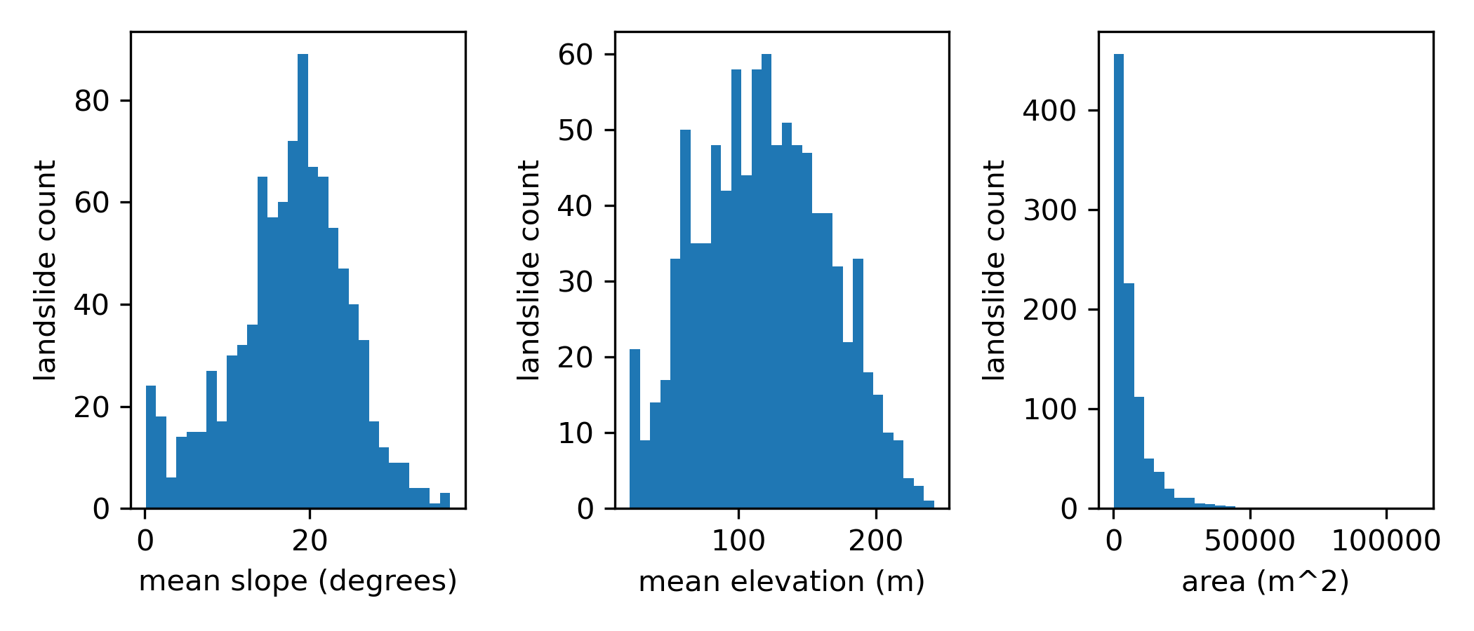
f, ax = plt.subplots(1, 3, figsize=(7, 3))
ax[0].hist(landslides_gdf.slope_mean, bins=30)
ax[0].set_xlabel('mean slope (degrees)')
ax[0].set_ylabel('landslide count')
ax[1].hist(landslides_gdf.elevation_mean, bins=30)
ax[1].set_xlabel('mean elevation (m)')
ax[1].set_ylabel('landslide count')
ax[2].hist(landslides_gdf.area, bins=30)
#ax[2].set_xscale('log')
ax[2].set_xlabel('area (m^2)')
ax[2].set_ylabel('landslide count')
plt.tight_layout()

f.savefig('imgs/landslide_histograms.png', dpi=300)

We now have a vector landslide inventory with area, slope, and elevation information for each landslide! Let’s save it to a geojson.

landslides_gdf.to_file(f'landslides_{earthquake_date}_{minx}_{miny}_{maxx}_{maxy}.geojson')

Part 3: Inventory accuracy (1 pt)#

To quantify the accuracy of our landslide dataset, let’s quickly compare it to a hand-drawn coseismic landslide inventory for this event. We’ll use the landslide inventory associated with Shang et al. (2019). Their data are available on Zenodo, so we can easily download them. Simply uncomment and run the following cell.

Zhang, S., Li, R., Wang, F., & Iio, A. (2019). Characteristics of landslides triggered by the 2018 Hokkaido Eastern Iburi earthquake, Northern Japan. Landslides, 16, 1691-1708.

# # download the hand-drawn inventory to the data folder
# !wget -P data https://zenodo.org/records/2577300/files/Iburi%20landslide%20dataset.zip

# # unzip the data
# !unzip data/Iburi\ landslide\ dataset.zip -d data

# load in the data
handdrawn_landslides_gdf = gpd.read_file('data/Iburi landslide dataset/landslide_inventory/landslide_inventory.shp')
# reproject to local UTM zone
handdrawn_landslides_gdf = handdrawn_landslides_gdf.to_crs(landslides_gdf.crs)
# clip to the bounds of our dataset for comparison
handdrawn_landslides_gdf = gpd.clip(handdrawn_landslides_gdf, landslides_gdf.total_bounds)

Create a plot showing our landslide inventory and the hand-drawn landslide inventory#

# STUDENT CODE HERE

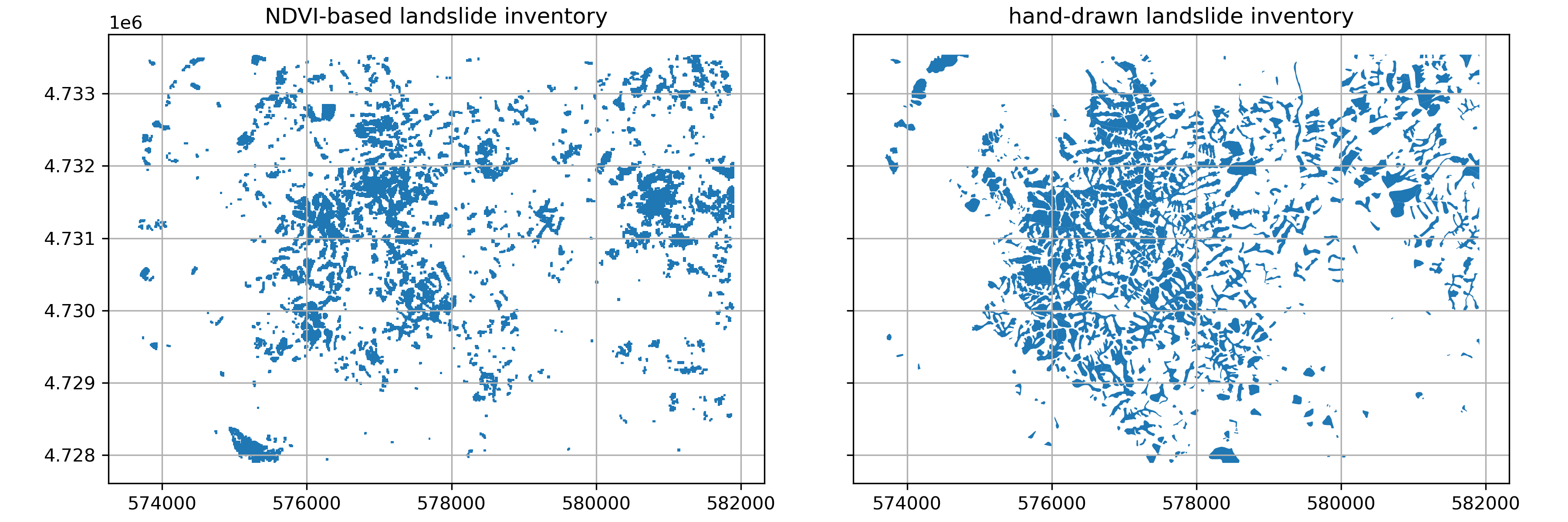
Written response: Compare and contrast our landslide inventory and the hand-drawn landslide inventory.#

Consider the advantages and drawbacks that each approach to generating products might have for helping with disaster response.

STUDENT WRITTEN RESPONSE HERE

To compute accuracy metrics for our dataset, we first need to convert the hand-drawn landslides inventory, which is a vector dataset, to a raster. We can do this using the rasterio.features.rasterize() function.

# rasterize the hand-drawn landslide polygons
handdrawn_raster = rasterize(
    [(geom, 1) for geom in handdrawn_landslides_gdf.geometry],  
    out_shape=s2_ds.landslide_id.shape,
    transform=s2_ds.rio.transform() ,
    fill=0,  # value to use for background
    dtype="uint8"
)

s2_ds = s2_ds.assign(handdrawn_landslides=(["y", "x"], handdrawn_raster))

Now we can compute some accuracy metrics for our inventory. Let’s start with intersection over union (IoU), a common metric used to assess performance in image segmentation tasks. This computes the area that our two inventories overlap (intersection) divided by the total area of both inventories (union)

intersection = np.logical_and(s2_ds.landslide_mask_cleaned, s2_ds.handdrawn_landslides).sum()  # true positives
union = np.logical_or(s2_ds.landslide_mask_cleaned, s2_ds.handdrawn_landslides).sum()  # union of both masks
iou = intersection / union if union > 0 else 0  # IoU score

print(f"Intersection over Union (IoU): {iou:.3f}")

Intersection over Union (IoU): 0.387

Now let’s compute precision and recall. Precision is a measure of how much of the area classified as landslide is actually landslide, and recall is measure of how much of the total landslide area we were able to identify. Finally, F1 score combines precision and recall into a single metric.

# true positives (correctly detected landslides)
TP = np.logical_and(s2_ds.landslide_mask_cleaned, s2_ds.handdrawn_landslides).sum()

# false positives (detected landslides not in inventory)
FP = np.logical_and(s2_ds.landslide_mask_cleaned, ~s2_ds.handdrawn_landslides).sum()

# false negatives (inventory landslides not detected)
FN = np.logical_and(~s2_ds.landslide_mask_cleaned, s2_ds.handdrawn_landslides).sum()

# precision, recall, and F1-score
precision = TP / (TP + FP) if (TP + FP) > 0 else 0
recall = TP / (TP + FN) if (TP + FN) > 0 else 0
f1_score = 2 * (precision * recall) / (precision + recall) if (precision + recall) > 0 else 0

print(f"Precision: {precision:.3f}")
print(f"Recall: {recall:.3f}")
print(f"F1 Score: {f1_score:.3f}")

Precision: 0.393
Recall: 0.490
F1 Score: 0.436

Written Response: Interpret these performance metrics#

Does our inventory contain more false positives or false negatives?
Imagine you provide this inventory to a disaster response team. When asked, “How good is this inventory?”, how would you respond?

STUDENT WRITTEN RESPONSE HERE

Great work, you finished Notebook 1! Move on to Notebook #2, but first…#

Save this notebook!
- You can also do an add, commit, and push at this stage
Shut down the kernel to free RAM
Proceed to Notebook #2!

Lab 09 assignment notebook 1 (20 pts)

Contents

Lab 09 assignment notebook 1 (20 pts)#

Introduction#

Objectives#

Instructions#

Background#

Part 1: Loading data (4 pts)#

1.1 Seasonal NDVI#

Query the Planetary Computer STAC catalog to find Sentinel-2 Level 2A data prior to the earthquake for our area of interest.#

Use `odc-stac` to load these items into an Xarray dataset called `pre_earthquake_s2_ds`.#

Compute median seasonal NDVI#

Plot median NDVI for each month#

Written Response: Describe the seasonal evolution of NDVI at this location and speculate about what might cause it.#

1.2 NDVI time series#

Query the Planetary Computer STAC catalog for Sentinel-2 images within our date range for our area of interest#

Use `odc-stac` to load the data into an Xarray dataset called `s2_ds`#

Use the `s2_ds` Dataset to create a figure with the following 6 panels:#

Written Response: Take a moment to consider these plots.#

1.3 Copernicus 30m DEM#

Bring in a DEM for our area of interest.#

Part 2: Fitting a step function, landslide classification, generating a landslide inventory (3 pts)#

2.1 Fitting a step function#

Create a plot with three panels:#

Written Response: Consider these plots.#

2.2 Classifying landslides#

Create a plot that shows your mask next to the raster that it’s based on.#

2.3 Segmenting landslides#

2.4 Polygonizing landslides and calculating zonal statistics#

Written Response: Consider the landslide inventory.#

Plot the landslide inventory on top of the DEM DataArray we pulled in in Part 1.#

Part 3: Inventory accuracy (1 pt)#

Create a plot showing our landslide inventory and the hand-drawn landslide inventory#

Written response: Compare and contrast our landslide inventory and the hand-drawn landslide inventory.#

Written Response: Interpret these performance metrics#

Great work, you finished Notebook 1! Move on to Notebook #2, but first…#

Lab 09 assignment notebook 1 (20 pts)

Contents

Lab 09 assignment notebook 1 (20 pts)#

Introduction#

Objectives#

Instructions#

Background#

Part 0: Defining variables related to the 2018 Hokkaido Eastern Iburi earthquake#

Part 1: Loading data (4 pts)#

1.1 Seasonal NDVI#

Query the Planetary Computer STAC catalog to find Sentinel-2 Level 2A data prior to the earthquake for our area of interest.#

Use odc-stac to load these items into an Xarray dataset called pre_earthquake_s2_ds.#

Compute median seasonal NDVI#

Plot median NDVI for each month#

Written Response: Describe the seasonal evolution of NDVI at this location and speculate about what might cause it.#

1.2 NDVI time series#

Query the Planetary Computer STAC catalog for Sentinel-2 images within our date range for our area of interest#

Use odc-stac to load the data into an Xarray dataset called s2_ds#

Use the s2_ds Dataset to create a figure with the following 6 panels:#

Written Response: Take a moment to consider these plots.#

1.3 Copernicus 30m DEM#

Bring in a DEM for our area of interest.#

Part 2: Fitting a step function, landslide classification, generating a landslide inventory (3 pts)#

2.1 Fitting a step function#

Create a plot with three panels:#

Written Response: Consider these plots.#

2.2 Classifying landslides#

Create a plot that shows your mask next to the raster that it’s based on.#

2.3 Segmenting landslides#

2.4 Polygonizing landslides and calculating zonal statistics#

Written Response: Consider the landslide inventory.#

Plot the landslide inventory on top of the DEM DataArray we pulled in in Part 1.#

Part 3: Inventory accuracy (1 pt)#

Create a plot showing our landslide inventory and the hand-drawn landslide inventory#

Written response: Compare and contrast our landslide inventory and the hand-drawn landslide inventory.#

Written Response: Interpret these performance metrics#

Great work, you finished Notebook 1! Move on to Notebook #2, but first…#

Use `odc-stac` to load these items into an Xarray dataset called `pre_earthquake_s2_ds`.#

Use `odc-stac` to load the data into an Xarray dataset called `s2_ds`#

Use the `s2_ds` Dataset to create a figure with the following 6 panels:#