09 APIs and STAC Catalogs demo#
UW Geospatial Data Analysis
CEE467/CEWA567
David Shean, Eric Gagliano, Quinn Brencher
Overview#
In this notebook, we’ll explore:
Web APIs and why they matter for geospatial data
Accessing catalogs with pystac_client and the STAC API
Loading and visualizing nDarray satellite image data using odc-stac
1. APIs and Python#
Read about APIs on the prep page! There we introduced the API we’ll be querying from Open-Meteo.
See how an API request changes depending on what you’re asking for…#
Check out the open-meteo documentation. Scroll down to right underneath the chart and take note of the API url and its parameters. Now scroll back up, change the selections, and scroll back down to see how the url has changed.
Here’s an example of a basic API request using the requests library: We’ll send an API request to Open-Meteo’s API, an open source weather data provider#
# very common to use requests library for making HTTP requests
import requests
# notice that the response says 200 -- what does this mean again?
response = requests.get("https://api.open-meteo.com/v1/forecast?latitude=47.6&longitude=-122.3¤t_weather=true")
response
<Response [200]>
# what does the reponse look like? follow the url!
response.request.url
'https://api.open-meteo.com/v1/forecast?latitude=47.6&longitude=-122.3¤t_weather=true'
# now we'll want to use the .json() method to get the data
data = response.json()
data
{'latitude': 47.60265,
'longitude': -122.28637,
'generationtime_ms': 0.0692605972290039,
'utc_offset_seconds': 0,
'timezone': 'GMT',
'timezone_abbreviation': 'GMT',
'elevation': 93.0,
'current_weather_units': {'time': 'iso8601',
'interval': 'seconds',
'temperature': '°C',
'windspeed': 'km/h',
'winddirection': '°',
'is_day': '',
'weathercode': 'wmo code'},
'current_weather': {'time': '2025-03-04T03:00',
'interval': 900,
'temperature': 8.5,
'windspeed': 8.2,
'winddirection': 229,
'is_day': 0,
'weathercode': 3}}
# Display the results
print(f"Temperature in Seattle: {data['current_weather']['temperature']}°C")
print(f"Wind speed: {data['current_weather']['windspeed']} km/h")
print(f"Time of observation: {data['current_weather']['time']}")
Temperature in Seattle: 8.5°C
Wind speed: 8.2 km/h
Time of observation: 2025-03-04T03:00
What if we tried with an invalid request?#
try:
# Bad request with invalid parameters
bad_response = requests.get("https://api.open-meteo.com/v1/forecast?latitude=999&longitude=-999")
# Check if the request was successful
bad_response.raise_for_status()
except requests.exceptions.HTTPError as err:
print(f"HTTP Error occurred: {err}")
print(f"Response body: {bad_response.text}")
HTTP Error occurred: 400 Client Error: Bad Request for url: https://api.open-meteo.com/v1/forecast?latitude=999&longitude=-999
Response body: {"error":true,"reason":"Latitude must be in range of -90 to 90°. Given: 999.0."}
Now let’s try an API focused on Geospatial data! We’ll try out the Overpass API that will allow us to access OpenStreetMap data#
def query_overpass(query):
overpass_url = "https://overpass-api.de/api/interpreter"
response = requests.get(overpass_url, params={'data': query})
return response
query = """
[out:json];
// Define our search area
area["name"="University of Washington"]->.searchArea;
// Find all "restaurants in this area
node["amenity"="restaurant"](area.searchArea);
// Output all data for these nodes
out body;
"""
response = query_overpass(query)
response
<Response [200]>
result = response.json()
result
{'version': 0.6,
'generator': 'Overpass API 0.7.62.5 1bd436f1',
'osm3s': {'timestamp_osm_base': '2025-03-04T03:02:45Z',
'timestamp_areas_base': '2024-12-31T00:49:33Z',
'copyright': 'The data included in this document is from www.openstreetmap.org. The data is made available under ODbL.'},
'elements': [{'type': 'node',
'id': 2671015705,
'lat': 47.6517371,
'lon': -122.3132664,
'tags': {'amenity': 'restaurant',
'cuisine': 'sandwich',
'name': 'Vista Café',
'opening_hours': 'Mo-Fr 07:30-15:00',
'website': 'https://www.hfs.washington.edu/dining/Default.aspx?id=324'}},
{'type': 'node',
'id': 2995199840,
'lat': 47.649378,
'lon': -122.3077192,
'tags': {'addr:city': 'Seattle',
'addr:housenumber': '1959',
'addr:postcode': '98195',
'addr:street': 'Northeast Pacific Street',
'amenity': 'restaurant',
'name': 'Plaza Cafe',
'source:addr:id': '14021'}},
{'type': 'node',
'id': 3355097453,
'lat': 47.6566177,
'lon': -122.3148405,
'tags': {'addr:city': 'Seattle',
'addr:housenumber': '1218',
'addr:postcode': '98105',
'addr:state': 'WA',
'addr:street': 'Northeast Campus Parkway',
'amenity': 'restaurant',
'cuisine': 'american',
'name': 'Cultivate'}},
{'type': 'node',
'id': 6437270427,
'lat': 47.6596297,
'lon': -122.304489,
'tags': {'addr:city': 'Seattle',
'addr:housenumber': '4294',
'addr:postcode': '98195',
'addr:state': 'WA',
'addr:street': 'Little Canoe Channel Northeast',
'addr:unit': '202',
'amenity': 'restaurant',
'branch': 'Willow Hall',
'brand': 'Pagliacci Pizza',
'brand:wikidata': 'Q7124370',
'cuisine': 'pizza',
'diet:vegan': 'yes',
'diet:vegetarian': 'yes',
'level': '1',
'name': 'Pagliacci Pizza',
'opening_hours': 'Mo-Th 15:00-21:00; Fr 15:00-20:00',
'takeaway': 'yes',
'website': 'https://www.pagliacci.com/location/willow-hall'}}]}
import shapely
import geopandas as gpd
import matplotlib.pyplot as plt
import contextily as ctx
# Process results into a GeoDataFrame
restaurant = []
for element in result['elements']:
if element['type'] == 'node':
cafe = {
'id': element['id'],
'name': element.get('tags', {}).get('name', 'Unnamed'),
'geometry': shapely.geometry.Point(element['lon'], element['lat'])
}
restaurant.append(cafe)
restaurant_gdf = gpd.GeoDataFrame(restaurant, crs="EPSG:4326")
restaurant_gdf
| id | name | geometry | |
|---|---|---|---|
| 0 | 2671015705 | Vista Café | POINT (-122.31327 47.65174) |
| 1 | 2995199840 | Plaza Cafe | POINT (-122.30772 47.64938) |
| 2 | 3355097453 | Cultivate | POINT (-122.31484 47.65662) |
| 3 | 6437270427 | Pagliacci Pizza | POINT (-122.30449 47.65963) |
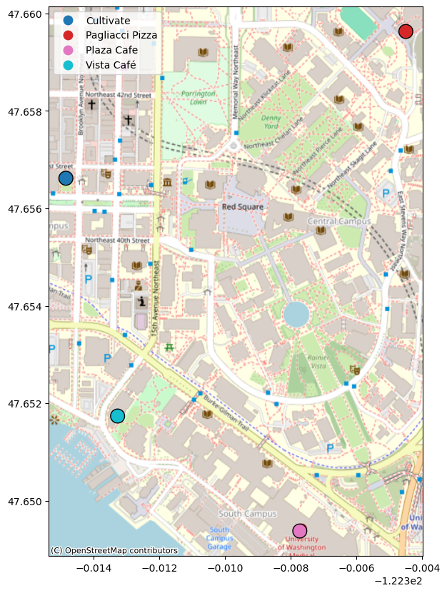
f,ax=plt.subplots(figsize=(10,10))
restaurant_gdf.plot(ax=ax, column='name', categorical=True, legend=True, legend_kwds={'loc': 'upper left'}, edgecolor='black', markersize=200)
ctx.add_basemap(ax, crs=restaurant_gdf.crs, source=ctx.providers.OpenStreetMap.Mapnik)
Or we could have used osmnx, a python package that makes API requests to OpenStreetMap easier#
import osmnx
uw_gdf = osmnx.geocode_to_gdf("University of Washington, Seattle, WA")
uw_gdf
| geometry | bbox_west | bbox_south | bbox_east | bbox_north | place_id | osm_type | osm_id | lat | lon | class | type | place_rank | importance | addresstype | name | display_name | |
|---|---|---|---|---|---|---|---|---|---|---|---|---|---|---|---|---|---|
| 0 | MULTIPOLYGON (((-122.32181 47.65497, -122.3217... | -122.321808 | 47.647782 | -122.287588 | 47.666072 | 301152014 | relation | 5268488 | 47.65543 | -122.300169 | amenity | university | 30 | 0.65117 | amenity | University of Washington | University of Washington, 9th Avenue Northeast... |
wilcox_hall_gdf = osmnx.geocode_to_gdf("2117 Mason Rd, Seattle, WA 98195")
walk_network = osmnx.graph_from_place("University of Washington, Seattle, WA", network_type="walk")
restaurants_gdf = osmnx.features.features_from_place("University of Washington, Seattle, WA", tags={'amenity': 'restaurant'})
restaurants_gdf
| geometry | addr:city | addr:housenumber | addr:postcode | addr:state | addr:street | amenity | cuisine | diet:vegan | diet:vegetarian | name | opening_hours | takeaway | website | level | addr:unit | branch | brand | brand:wikidata | source:addr:id | ||
|---|---|---|---|---|---|---|---|---|---|---|---|---|---|---|---|---|---|---|---|---|---|
| element | id | ||||||||||||||||||||
| node | 2671015705 | POINT (-122.31327 47.65174) | NaN | NaN | NaN | NaN | NaN | restaurant | sandwich | NaN | NaN | Vista Café | Mo-Fr 07:30-15:00 | NaN | https://www.hfs.washington.edu/dining/Default.... | NaN | NaN | NaN | NaN | NaN | NaN |
| 2995199840 | POINT (-122.30772 47.64938) | Seattle | 1959 | 98195 | NaN | Northeast Pacific Street | restaurant | NaN | NaN | NaN | Plaza Cafe | NaN | NaN | NaN | NaN | NaN | NaN | NaN | NaN | 14021 | |
| 3355097453 | POINT (-122.31484 47.65662) | Seattle | 1218 | 98105 | WA | Northeast Campus Parkway | restaurant | american | NaN | NaN | Cultivate | NaN | NaN | NaN | NaN | NaN | NaN | NaN | NaN | NaN | |
| 6437270427 | POINT (-122.30449 47.65963) | Seattle | 4294 | 98195 | WA | Little Canoe Channel Northeast | restaurant | pizza | yes | yes | Pagliacci Pizza | Mo-Th 15:00-21:00; Fr 15:00-20:00 | yes | https://www.pagliacci.com/location/willow-hall | 1 | 202 | Willow Hall | Pagliacci Pizza | Q7124370 | NaN |
f,ax=plt.subplots(figsize=(10,10))
uw_gdf.plot(ax=ax, facecolor='none', edgecolor='purple', linewidth=5)
osmnx.convert.graph_to_gdfs(walk_network, nodes=False, edges=True).plot(ax=ax, linewidth=0.5, edgecolor='black')
wilcox_hall_gdf.plot(ax=ax, color='red', zorder=4)
restaurant_gdf.plot(ax=ax, column='name', categorical=True, legend=True, legend_kwds={'loc': 'upper left'}, edgecolor='black', markersize=200, zorder=5)
ctx.add_basemap(ax, crs=uw_gdf.crs, source=ctx.providers.OpenStreetMap.Mapnik)
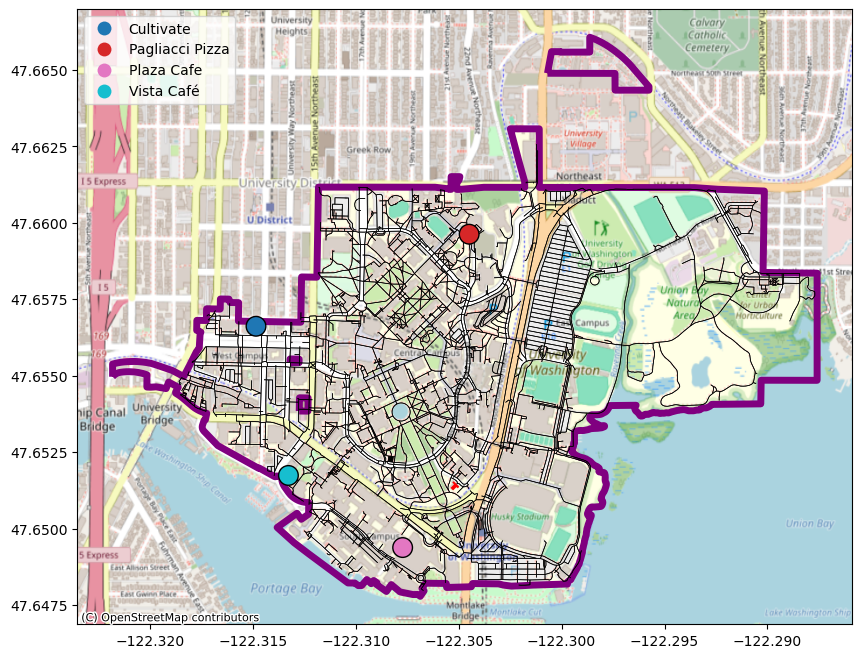
We could even use the walk network to find which place Eric can grab lunch fastest from! See graph network, routing, and travel time examples here.
2. Querying STAC catalogs#
Microsoft’s Planetary Computer is one of many platforms that host a variety of Earth observation datasets accompanied by a STAC catalog to access them. Check out Reading Data from the STAC API for more info. We’ll be looking at their Sentinel-2 dataset for the rest of this demo.
Let’s try to access Microsoft Planetary Computer’s Sentinel-2 STAC catalog#
We’ll use pystac_client to open the STAC catalog#
import pystac_client
import planetary_computer
catalog = pystac_client.Client.open(
"https://planetarycomputer.microsoft.com/api/stac/v1",
modifier=planetary_computer.sign_inplace,
)
#catalog = pystac_client.Client.open("https://earth-search.aws.element84.com/v1/") #another catalog option for Sentinel-2
catalog
- type "Catalog"
- id "microsoft-pc"
- stac_version "1.1.0"
- description "Searchable spatiotemporal metadata describing Earth science datasets hosted by the Microsoft Planetary Computer"
links[] 133 items
0
- rel "self"
- href "https://planetarycomputer.microsoft.com/api/stac/v1"
- type "application/json"
1
- rel "root"
- href "https://planetarycomputer.microsoft.com/api/stac/v1/"
- type "application/json"
2
- rel "data"
- href "https://planetarycomputer.microsoft.com/api/stac/v1/collections"
- type "application/json"
3
- rel "conformance"
- href "https://planetarycomputer.microsoft.com/api/stac/v1/conformance"
- type "application/json"
- title "STAC/OGC conformance classes implemented by this server"
4
- rel "search"
- href "https://planetarycomputer.microsoft.com/api/stac/v1/search"
- type "application/geo+json"
- title "STAC search"
- method "GET"
5
- rel "search"
- href "https://planetarycomputer.microsoft.com/api/stac/v1/search"
- type "application/geo+json"
- title "STAC search"
- method "POST"
6
- rel "http://www.opengis.net/def/rel/ogc/1.0/queryables"
- href "https://planetarycomputer.microsoft.com/api/stac/v1/queryables"
- type "application/schema+json"
- title "Queryables"
- method "GET"
7
- rel "child"
- href "https://planetarycomputer.microsoft.com/api/stac/v1/collections/daymet-annual-pr"
- type "application/json"
- title "Daymet Annual Puerto Rico"
8
- rel "child"
- href "https://planetarycomputer.microsoft.com/api/stac/v1/collections/daymet-daily-hi"
- type "application/json"
- title "Daymet Daily Hawaii"
9
- rel "child"
- href "https://planetarycomputer.microsoft.com/api/stac/v1/collections/3dep-seamless"
- type "application/json"
- title "USGS 3DEP Seamless DEMs"
10
- rel "child"
- href "https://planetarycomputer.microsoft.com/api/stac/v1/collections/3dep-lidar-dsm"
- type "application/json"
- title "USGS 3DEP Lidar Digital Surface Model"
11
- rel "child"
- href "https://planetarycomputer.microsoft.com/api/stac/v1/collections/fia"
- type "application/json"
- title "Forest Inventory and Analysis"
12
- rel "child"
- href "https://planetarycomputer.microsoft.com/api/stac/v1/collections/sentinel-1-rtc"
- type "application/json"
- title "Sentinel 1 Radiometrically Terrain Corrected (RTC)"
13
- rel "child"
- href "https://planetarycomputer.microsoft.com/api/stac/v1/collections/gridmet"
- type "application/json"
- title "gridMET"
14
- rel "child"
- href "https://planetarycomputer.microsoft.com/api/stac/v1/collections/daymet-annual-na"
- type "application/json"
- title "Daymet Annual North America"
15
- rel "child"
- href "https://planetarycomputer.microsoft.com/api/stac/v1/collections/daymet-monthly-na"
- type "application/json"
- title "Daymet Monthly North America"
16
- rel "child"
- href "https://planetarycomputer.microsoft.com/api/stac/v1/collections/daymet-annual-hi"
- type "application/json"
- title "Daymet Annual Hawaii"
17
- rel "child"
- href "https://planetarycomputer.microsoft.com/api/stac/v1/collections/daymet-monthly-hi"
- type "application/json"
- title "Daymet Monthly Hawaii"
18
- rel "child"
- href "https://planetarycomputer.microsoft.com/api/stac/v1/collections/daymet-monthly-pr"
- type "application/json"
- title "Daymet Monthly Puerto Rico"
19
- rel "child"
- href "https://planetarycomputer.microsoft.com/api/stac/v1/collections/gnatsgo-tables"
- type "application/json"
- title "gNATSGO Soil Database - Tables"
20
- rel "child"
- href "https://planetarycomputer.microsoft.com/api/stac/v1/collections/hgb"
- type "application/json"
- title "HGB: Harmonized Global Biomass for 2010"
21
- rel "child"
- href "https://planetarycomputer.microsoft.com/api/stac/v1/collections/cop-dem-glo-30"
- type "application/json"
- title "Copernicus DEM GLO-30"
22
- rel "child"
- href "https://planetarycomputer.microsoft.com/api/stac/v1/collections/cop-dem-glo-90"
- type "application/json"
- title "Copernicus DEM GLO-90"
23
- rel "child"
- href "https://planetarycomputer.microsoft.com/api/stac/v1/collections/goes-cmi"
- type "application/json"
- title "GOES-R Cloud & Moisture Imagery"
24
- rel "child"
- href "https://planetarycomputer.microsoft.com/api/stac/v1/collections/terraclimate"
- type "application/json"
- title "TerraClimate"
25
- rel "child"
- href "https://planetarycomputer.microsoft.com/api/stac/v1/collections/nasa-nex-gddp-cmip6"
- type "application/json"
- title "Earth Exchange Global Daily Downscaled Projections (NEX-GDDP-CMIP6)"
26
- rel "child"
- href "https://planetarycomputer.microsoft.com/api/stac/v1/collections/gpm-imerg-hhr"
- type "application/json"
- title "GPM IMERG"
27
- rel "child"
- href "https://planetarycomputer.microsoft.com/api/stac/v1/collections/gnatsgo-rasters"
- type "application/json"
- title "gNATSGO Soil Database - Rasters"
28
- rel "child"
- href "https://planetarycomputer.microsoft.com/api/stac/v1/collections/3dep-lidar-hag"
- type "application/json"
- title "USGS 3DEP Lidar Height above Ground"
29
- rel "child"
- href "https://planetarycomputer.microsoft.com/api/stac/v1/collections/io-lulc-annual-v02"
- type "application/json"
- title "10m Annual Land Use Land Cover (9-class) V2"
30
- rel "child"
- href "https://planetarycomputer.microsoft.com/api/stac/v1/collections/conus404"
- type "application/json"
- title "CONUS404"
31
- rel "child"
- href "https://planetarycomputer.microsoft.com/api/stac/v1/collections/3dep-lidar-intensity"
- type "application/json"
- title "USGS 3DEP Lidar Intensity"
32
- rel "child"
- href "https://planetarycomputer.microsoft.com/api/stac/v1/collections/3dep-lidar-pointsourceid"
- type "application/json"
- title "USGS 3DEP Lidar Point Source"
33
- rel "child"
- href "https://planetarycomputer.microsoft.com/api/stac/v1/collections/mtbs"
- type "application/json"
- title "MTBS: Monitoring Trends in Burn Severity"
34
- rel "child"
- href "https://planetarycomputer.microsoft.com/api/stac/v1/collections/noaa-c-cap"
- type "application/json"
- title "C-CAP Regional Land Cover and Change"
35
- rel "child"
- href "https://planetarycomputer.microsoft.com/api/stac/v1/collections/3dep-lidar-copc"
- type "application/json"
- title "USGS 3DEP Lidar Point Cloud"
36
- rel "child"
- href "https://planetarycomputer.microsoft.com/api/stac/v1/collections/modis-64A1-061"
- type "application/json"
- title "MODIS Burned Area Monthly"
37
- rel "child"
- href "https://planetarycomputer.microsoft.com/api/stac/v1/collections/alos-fnf-mosaic"
- type "application/json"
- title "ALOS Forest/Non-Forest Annual Mosaic"
38
- rel "child"
- href "https://planetarycomputer.microsoft.com/api/stac/v1/collections/3dep-lidar-returns"
- type "application/json"
- title "USGS 3DEP Lidar Returns"
39
- rel "child"
- href "https://planetarycomputer.microsoft.com/api/stac/v1/collections/mobi"
- type "application/json"
- title "MoBI: Map of Biodiversity Importance"
40
- rel "child"
- href "https://planetarycomputer.microsoft.com/api/stac/v1/collections/landsat-c2-l2"
- type "application/json"
- title "Landsat Collection 2 Level-2"
41
- rel "child"
- href "https://planetarycomputer.microsoft.com/api/stac/v1/collections/era5-pds"
- type "application/json"
- title "ERA5 - PDS"
42
- rel "child"
- href "https://planetarycomputer.microsoft.com/api/stac/v1/collections/chloris-biomass"
- type "application/json"
- title "Chloris Biomass"
43
- rel "child"
- href "https://planetarycomputer.microsoft.com/api/stac/v1/collections/kaza-hydroforecast"
- type "application/json"
- title "HydroForecast - Kwando & Upper Zambezi Rivers"
44
- rel "child"
- href "https://planetarycomputer.microsoft.com/api/stac/v1/collections/planet-nicfi-analytic"
- type "application/json"
- title "Planet-NICFI Basemaps (Analytic)"
45
- rel "child"
- href "https://planetarycomputer.microsoft.com/api/stac/v1/collections/modis-17A2H-061"
- type "application/json"
- title "MODIS Gross Primary Productivity 8-Day"
46
- rel "child"
- href "https://planetarycomputer.microsoft.com/api/stac/v1/collections/modis-11A2-061"
- type "application/json"
- title "MODIS Land Surface Temperature/Emissivity 8-Day"
47
- rel "child"
- href "https://planetarycomputer.microsoft.com/api/stac/v1/collections/daymet-daily-pr"
- type "application/json"
- title "Daymet Daily Puerto Rico"
48
- rel "child"
- href "https://planetarycomputer.microsoft.com/api/stac/v1/collections/3dep-lidar-dtm-native"
- type "application/json"
- title "USGS 3DEP Lidar Digital Terrain Model (Native)"
49
- rel "child"
- href "https://planetarycomputer.microsoft.com/api/stac/v1/collections/3dep-lidar-classification"
- type "application/json"
- title "USGS 3DEP Lidar Classification"
50
- rel "child"
- href "https://planetarycomputer.microsoft.com/api/stac/v1/collections/3dep-lidar-dtm"
- type "application/json"
- title "USGS 3DEP Lidar Digital Terrain Model"
51
- rel "child"
- href "https://planetarycomputer.microsoft.com/api/stac/v1/collections/gap"
- type "application/json"
- title "USGS Gap Land Cover"
52
- rel "child"
- href "https://planetarycomputer.microsoft.com/api/stac/v1/collections/modis-17A2HGF-061"
- type "application/json"
- title "MODIS Gross Primary Productivity 8-Day Gap-Filled"
53
- rel "child"
- href "https://planetarycomputer.microsoft.com/api/stac/v1/collections/planet-nicfi-visual"
- type "application/json"
- title "Planet-NICFI Basemaps (Visual)"
54
- rel "child"
- href "https://planetarycomputer.microsoft.com/api/stac/v1/collections/gbif"
- type "application/json"
- title "Global Biodiversity Information Facility (GBIF)"
55
- rel "child"
- href "https://planetarycomputer.microsoft.com/api/stac/v1/collections/modis-17A3HGF-061"
- type "application/json"
- title "MODIS Net Primary Production Yearly Gap-Filled"
56
- rel "child"
- href "https://planetarycomputer.microsoft.com/api/stac/v1/collections/modis-09A1-061"
- type "application/json"
- title "MODIS Surface Reflectance 8-Day (500m)"
57
- rel "child"
- href "https://planetarycomputer.microsoft.com/api/stac/v1/collections/alos-dem"
- type "application/json"
- title "ALOS World 3D-30m"
58
- rel "child"
- href "https://planetarycomputer.microsoft.com/api/stac/v1/collections/alos-palsar-mosaic"
- type "application/json"
- title "ALOS PALSAR Annual Mosaic"
59
- rel "child"
- href "https://planetarycomputer.microsoft.com/api/stac/v1/collections/deltares-water-availability"
- type "application/json"
- title "Deltares Global Water Availability"
60
- rel "child"
- href "https://planetarycomputer.microsoft.com/api/stac/v1/collections/modis-16A3GF-061"
- type "application/json"
- title "MODIS Net Evapotranspiration Yearly Gap-Filled"
61
- rel "child"
- href "https://planetarycomputer.microsoft.com/api/stac/v1/collections/modis-21A2-061"
- type "application/json"
- title "MODIS Land Surface Temperature/3-Band Emissivity 8-Day"
62
- rel "child"
- href "https://planetarycomputer.microsoft.com/api/stac/v1/collections/us-census"
- type "application/json"
- title "US Census"
63
- rel "child"
- href "https://planetarycomputer.microsoft.com/api/stac/v1/collections/jrc-gsw"
- type "application/json"
- title "JRC Global Surface Water"
64
- rel "child"
- href "https://planetarycomputer.microsoft.com/api/stac/v1/collections/deltares-floods"
- type "application/json"
- title "Deltares Global Flood Maps"
65
- rel "child"
- href "https://planetarycomputer.microsoft.com/api/stac/v1/collections/modis-43A4-061"
- type "application/json"
- title "MODIS Nadir BRDF-Adjusted Reflectance (NBAR) Daily"
66
- rel "child"
- href "https://planetarycomputer.microsoft.com/api/stac/v1/collections/modis-09Q1-061"
- type "application/json"
- title "MODIS Surface Reflectance 8-Day (250m)"
67
- rel "child"
- href "https://planetarycomputer.microsoft.com/api/stac/v1/collections/modis-14A1-061"
- type "application/json"
- title "MODIS Thermal Anomalies/Fire Daily"
68
- rel "child"
- href "https://planetarycomputer.microsoft.com/api/stac/v1/collections/hrea"
- type "application/json"
- title "HREA: High Resolution Electricity Access"
69
- rel "child"
- href "https://planetarycomputer.microsoft.com/api/stac/v1/collections/modis-13Q1-061"
- type "application/json"
- title "MODIS Vegetation Indices 16-Day (250m)"
70
- rel "child"
- href "https://planetarycomputer.microsoft.com/api/stac/v1/collections/modis-14A2-061"
- type "application/json"
- title "MODIS Thermal Anomalies/Fire 8-Day"
71
- rel "child"
- href "https://planetarycomputer.microsoft.com/api/stac/v1/collections/sentinel-2-l2a"
- type "application/json"
- title "Sentinel-2 Level-2A"
72
- rel "child"
- href "https://planetarycomputer.microsoft.com/api/stac/v1/collections/modis-15A2H-061"
- type "application/json"
- title "MODIS Leaf Area Index/FPAR 8-Day"
73
- rel "child"
- href "https://planetarycomputer.microsoft.com/api/stac/v1/collections/modis-11A1-061"
- type "application/json"
- title "MODIS Land Surface Temperature/Emissivity Daily"
74
- rel "child"
- href "https://planetarycomputer.microsoft.com/api/stac/v1/collections/modis-15A3H-061"
- type "application/json"
- title "MODIS Leaf Area Index/FPAR 4-Day"
75
- rel "child"
- href "https://planetarycomputer.microsoft.com/api/stac/v1/collections/modis-13A1-061"
- type "application/json"
- title "MODIS Vegetation Indices 16-Day (500m)"
76
- rel "child"
- href "https://planetarycomputer.microsoft.com/api/stac/v1/collections/daymet-daily-na"
- type "application/json"
- title "Daymet Daily North America"
77
- rel "child"
- href "https://planetarycomputer.microsoft.com/api/stac/v1/collections/nrcan-landcover"
- type "application/json"
- title "Land Cover of Canada"
78
- rel "child"
- href "https://planetarycomputer.microsoft.com/api/stac/v1/collections/modis-10A2-061"
- type "application/json"
- title "MODIS Snow Cover 8-day"
79
- rel "child"
- href "https://planetarycomputer.microsoft.com/api/stac/v1/collections/ecmwf-forecast"
- type "application/json"
- title "ECMWF Open Data (real-time)"
80
- rel "child"
- href "https://planetarycomputer.microsoft.com/api/stac/v1/collections/noaa-mrms-qpe-24h-pass2"
- type "application/json"
- title "NOAA MRMS QPE 24-Hour Pass 2"
81
- rel "child"
- href "https://planetarycomputer.microsoft.com/api/stac/v1/collections/sentinel-1-grd"
- type "application/json"
- title "Sentinel 1 Level-1 Ground Range Detected (GRD)"
82
- rel "child"
- href "https://planetarycomputer.microsoft.com/api/stac/v1/collections/nasadem"
- type "application/json"
- title "NASADEM HGT v001"
83
- rel "child"
- href "https://planetarycomputer.microsoft.com/api/stac/v1/collections/io-lulc"
- type "application/json"
- title "Esri 10-Meter Land Cover (10-class)"
84
- rel "child"
- href "https://planetarycomputer.microsoft.com/api/stac/v1/collections/landsat-c2-l1"
- type "application/json"
- title "Landsat Collection 2 Level-1"
85
- rel "child"
- href "https://planetarycomputer.microsoft.com/api/stac/v1/collections/drcog-lulc"
- type "application/json"
- title "Denver Regional Council of Governments Land Use Land Cover"
86
- rel "child"
- href "https://planetarycomputer.microsoft.com/api/stac/v1/collections/chesapeake-lc-7"
- type "application/json"
- title "Chesapeake Land Cover (7-class)"
87
- rel "child"
- href "https://planetarycomputer.microsoft.com/api/stac/v1/collections/chesapeake-lc-13"
- type "application/json"
- title "Chesapeake Land Cover (13-class)"
88
- rel "child"
- href "https://planetarycomputer.microsoft.com/api/stac/v1/collections/chesapeake-lu"
- type "application/json"
- title "Chesapeake Land Use"
89
- rel "child"
- href "https://planetarycomputer.microsoft.com/api/stac/v1/collections/noaa-mrms-qpe-1h-pass1"
- type "application/json"
- title "NOAA MRMS QPE 1-Hour Pass 1"
90
- rel "child"
- href "https://planetarycomputer.microsoft.com/api/stac/v1/collections/noaa-mrms-qpe-1h-pass2"
- type "application/json"
- title "NOAA MRMS QPE 1-Hour Pass 2"
91
- rel "child"
- href "https://planetarycomputer.microsoft.com/api/stac/v1/collections/noaa-nclimgrid-monthly"
- type "application/json"
- title "Monthly NOAA U.S. Climate Gridded Dataset (NClimGrid)"
92
- rel "child"
- href "https://planetarycomputer.microsoft.com/api/stac/v1/collections/goes-glm"
- type "application/json"
- title "GOES-R Lightning Detection"
93
- rel "child"
- href "https://planetarycomputer.microsoft.com/api/stac/v1/collections/usda-cdl"
- type "application/json"
- title "USDA Cropland Data Layers (CDLs)"
94
- rel "child"
- href "https://planetarycomputer.microsoft.com/api/stac/v1/collections/eclipse"
- type "application/json"
- title "Urban Innovation Eclipse Sensor Data"
95
- rel "child"
- href "https://planetarycomputer.microsoft.com/api/stac/v1/collections/esa-cci-lc"
- type "application/json"
- title "ESA Climate Change Initiative Land Cover Maps (Cloud Optimized GeoTIFF)"
96
- rel "child"
- href "https://planetarycomputer.microsoft.com/api/stac/v1/collections/esa-cci-lc-netcdf"
- type "application/json"
- title "ESA Climate Change Initiative Land Cover Maps (NetCDF)"
97
- rel "child"
- href "https://planetarycomputer.microsoft.com/api/stac/v1/collections/fws-nwi"
- type "application/json"
- title "FWS National Wetlands Inventory"
98
- rel "child"
- href "https://planetarycomputer.microsoft.com/api/stac/v1/collections/usgs-lcmap-conus-v13"
- type "application/json"
- title "USGS LCMAP CONUS Collection 1.3"
99
- rel "child"
- href "https://planetarycomputer.microsoft.com/api/stac/v1/collections/usgs-lcmap-hawaii-v10"
- type "application/json"
- title "USGS LCMAP Hawaii Collection 1.0"
100
- rel "child"
- href "https://planetarycomputer.microsoft.com/api/stac/v1/collections/noaa-climate-normals-tabular"
- type "application/json"
- title "NOAA US Tabular Climate Normals"
101
- rel "child"
- href "https://planetarycomputer.microsoft.com/api/stac/v1/collections/noaa-climate-normals-netcdf"
- type "application/json"
- title "NOAA US Gridded Climate Normals (NetCDF)"
102
- rel "child"
- href "https://planetarycomputer.microsoft.com/api/stac/v1/collections/noaa-climate-normals-gridded"
- type "application/json"
- title "NOAA US Gridded Climate Normals (Cloud-Optimized GeoTIFF)"
103
- rel "child"
- href "https://planetarycomputer.microsoft.com/api/stac/v1/collections/aster-l1t"
- type "application/json"
- title "ASTER L1T"
104
- rel "child"
- href "https://planetarycomputer.microsoft.com/api/stac/v1/collections/cil-gdpcir-cc-by-sa"
- type "application/json"
- title "CIL Global Downscaled Projections for Climate Impacts Research (CC-BY-SA-4.0)"
105
- rel "child"
- href "https://planetarycomputer.microsoft.com/api/stac/v1/collections/naip"
- type "application/json"
- title "NAIP: National Agriculture Imagery Program"
106
- rel "child"
- href "https://planetarycomputer.microsoft.com/api/stac/v1/collections/io-lulc-9-class"
- type "application/json"
- title "10m Annual Land Use Land Cover (9-class) V1"
107
- rel "child"
- href "https://planetarycomputer.microsoft.com/api/stac/v1/collections/io-biodiversity"
- type "application/json"
- title "Biodiversity Intactness"
108
- rel "child"
- href "https://planetarycomputer.microsoft.com/api/stac/v1/collections/noaa-cdr-sea-surface-temperature-whoi"
- type "application/json"
- title "Sea Surface Temperature - WHOI CDR"
109
- rel "child"
- href "https://planetarycomputer.microsoft.com/api/stac/v1/collections/noaa-cdr-ocean-heat-content"
- type "application/json"
- title "Global Ocean Heat Content CDR"
110
- rel "child"
- href "https://planetarycomputer.microsoft.com/api/stac/v1/collections/cil-gdpcir-cc0"
- type "application/json"
- title "CIL Global Downscaled Projections for Climate Impacts Research (CC0-1.0)"
111
- rel "child"
- href "https://planetarycomputer.microsoft.com/api/stac/v1/collections/cil-gdpcir-cc-by"
- type "application/json"
- title "CIL Global Downscaled Projections for Climate Impacts Research (CC-BY-4.0)"
112
- rel "child"
- href "https://planetarycomputer.microsoft.com/api/stac/v1/collections/noaa-cdr-sea-surface-temperature-whoi-netcdf"
- type "application/json"
- title "Sea Surface Temperature - WHOI CDR NetCDFs"
113
- rel "child"
- href "https://planetarycomputer.microsoft.com/api/stac/v1/collections/noaa-cdr-sea-surface-temperature-optimum-interpolation"
- type "application/json"
- title "Sea Surface Temperature - Optimum Interpolation CDR"
114
- rel "child"
- href "https://planetarycomputer.microsoft.com/api/stac/v1/collections/modis-10A1-061"
- type "application/json"
- title "MODIS Snow Cover Daily"
115
- rel "child"
- href "https://planetarycomputer.microsoft.com/api/stac/v1/collections/sentinel-5p-l2-netcdf"
- type "application/json"
- title "Sentinel-5P Level-2"
116
- rel "child"
- href "https://planetarycomputer.microsoft.com/api/stac/v1/collections/sentinel-3-olci-wfr-l2-netcdf"
- type "application/json"
- title "Sentinel-3 Water (Full Resolution)"
117
- rel "child"
- href "https://planetarycomputer.microsoft.com/api/stac/v1/collections/noaa-cdr-ocean-heat-content-netcdf"
- type "application/json"
- title "Global Ocean Heat Content CDR NetCDFs"
118
- rel "child"
- href "https://planetarycomputer.microsoft.com/api/stac/v1/collections/sentinel-3-synergy-aod-l2-netcdf"
- type "application/json"
- title "Sentinel-3 Global Aerosol"
119
- rel "child"
- href "https://planetarycomputer.microsoft.com/api/stac/v1/collections/sentinel-3-synergy-v10-l2-netcdf"
- type "application/json"
- title "Sentinel-3 10-Day Surface Reflectance and NDVI (SPOT VEGETATION)"
120
- rel "child"
- href "https://planetarycomputer.microsoft.com/api/stac/v1/collections/sentinel-3-olci-lfr-l2-netcdf"
- type "application/json"
- title "Sentinel-3 Land (Full Resolution)"
121
- rel "child"
- href "https://planetarycomputer.microsoft.com/api/stac/v1/collections/sentinel-3-sral-lan-l2-netcdf"
- type "application/json"
- title "Sentinel-3 Land Radar Altimetry"
122
- rel "child"
- href "https://planetarycomputer.microsoft.com/api/stac/v1/collections/sentinel-3-slstr-lst-l2-netcdf"
- type "application/json"
- title "Sentinel-3 Land Surface Temperature"
123
- rel "child"
- href "https://planetarycomputer.microsoft.com/api/stac/v1/collections/sentinel-3-slstr-wst-l2-netcdf"
- type "application/json"
- title "Sentinel-3 Sea Surface Temperature"
124
- rel "child"
- href "https://planetarycomputer.microsoft.com/api/stac/v1/collections/sentinel-3-sral-wat-l2-netcdf"
- type "application/json"
- title "Sentinel-3 Ocean Radar Altimetry"
125
- rel "child"
- href "https://planetarycomputer.microsoft.com/api/stac/v1/collections/ms-buildings"
- type "application/json"
- title "Microsoft Building Footprints"
126
- rel "child"
- href "https://planetarycomputer.microsoft.com/api/stac/v1/collections/sentinel-3-slstr-frp-l2-netcdf"
- type "application/json"
- title "Sentinel-3 Fire Radiative Power"
127
- rel "child"
- href "https://planetarycomputer.microsoft.com/api/stac/v1/collections/sentinel-3-synergy-syn-l2-netcdf"
- type "application/json"
- title "Sentinel-3 Land Surface Reflectance and Aerosol"
128
- rel "child"
- href "https://planetarycomputer.microsoft.com/api/stac/v1/collections/sentinel-3-synergy-vgp-l2-netcdf"
- type "application/json"
- title "Sentinel-3 Top of Atmosphere Reflectance (SPOT VEGETATION)"
129
- rel "child"
- href "https://planetarycomputer.microsoft.com/api/stac/v1/collections/sentinel-3-synergy-vg1-l2-netcdf"
- type "application/json"
- title "Sentinel-3 1-Day Surface Reflectance and NDVI (SPOT VEGETATION)"
130
- rel "child"
- href "https://planetarycomputer.microsoft.com/api/stac/v1/collections/esa-worldcover"
- type "application/json"
- title "ESA WorldCover"
131
- rel "service-desc"
- href "https://planetarycomputer.microsoft.com/api/stac/v1/openapi.json"
- type "application/vnd.oai.openapi+json;version=3.0"
- title "OpenAPI service description"
132
- rel "service-doc"
- href "https://planetarycomputer.microsoft.com/api/stac/v1/docs"
- type "text/html"
- title "OpenAPI service documentation"
conformsTo[] 15 items
- 0 "https://api.stacspec.org/v1.0.0/core"
- 1 "http://www.opengis.net/spec/ogcapi-features-1/1.0/conf/oas30"
- 2 "https://api.stacspec.org/v1.0.0/item-search"
- 3 "https://api.stacspec.org/v1.0.0/item-search#query"
- 4 "https://api.stacspec.org/v1.0.0/item-search#fields"
- 5 "https://api.stacspec.org/v1.0.0/collections"
- 6 "http://www.opengis.net/spec/cql2/1.0/conf/basic-cql2"
- 7 "https://api.stacspec.org/v1.0.0/ogcapi-features"
- 8 "http://www.opengis.net/spec/cql2/1.0/conf/cql2-text"
- 9 "http://www.opengis.net/spec/ogcapi-features-3/1.0/conf/filter"
- 10 "https://api.stacspec.org/v1.0.0-rc.2/item-search#filter"
- 11 "https://api.stacspec.org/v1.0.0/item-search#sort"
- 12 "http://www.opengis.net/spec/cql2/1.0/conf/cql2-json"
- 13 "http://www.opengis.net/spec/ogcapi-features-1/1.0/conf/geojson"
- 14 "http://www.opengis.net/spec/ogcapi-features-1/1.0/conf/core"
- title "Microsoft Planetary Computer STAC API"
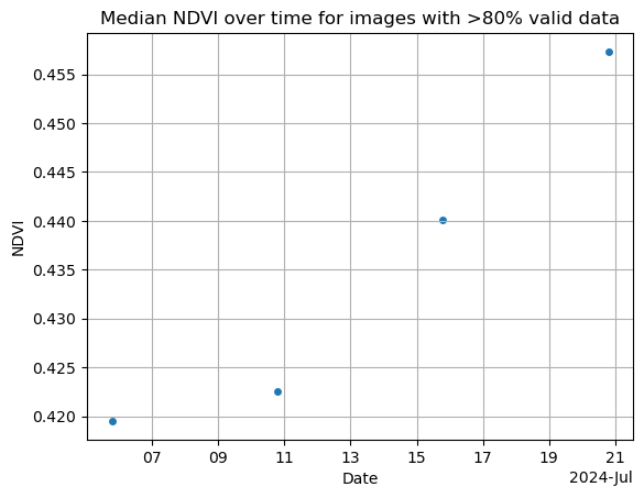
Now we’ll search the catalog with a date range and region of interest…#
start_date = "2024-07-15"
end_date = "2024-07-15"
states_gdf = gpd.read_file('http://eric.clst.org/assets/wiki/uploads/Stuff/gz_2010_us_040_00_5m.json')
wa_gdf = states_gdf[states_gdf['NAME'] == 'Washington']
bbox = wa_gdf.total_bounds
bbox
array([-124.733174, 45.543541, -116.915989, 49.002494])
search = catalog.search(
collections=["sentinel-2-l2a"], # sentinel-2-c1-l2a if using earthsearch
bbox=bbox,
datetime=(start_date, end_date),
#query={"eo:cloud_cover": {"lt": 30}},
)
Check out the items returned by the search!#
items = search.item_collection()
items
- type "FeatureCollection"
features[] 25 items
0
- type "Feature"
- stac_version "1.1.0"
stac_extensions[] 3 items
- 0 "https://stac-extensions.github.io/eo/v1.1.0/schema.json"
- 1 "https://stac-extensions.github.io/sat/v1.0.0/schema.json"
- 2 "https://stac-extensions.github.io/projection/v2.0.0/schema.json"
- id "S2A_MSIL2A_20240715T185921_R013_T11UMQ_20240716T032503"
geometry
- type "Polygon"
coordinates[] 1 items
0[] 12 items
0[] 2 items
- 0 -117.8722712
- 1 49.647203
1[] 2 items
- 0 -117.8839043
- 1 49.6218638
2[] 2 items
- 0 -117.9550421
- 1 49.4775563
3[] 2 items
- 0 -118.0237326
- 1 49.332698
4[] 2 items
- 0 -118.0927091
- 1 49.1880318
5[] 2 items
- 0 -118.1599354
- 1 49.0431102
6[] 2 items
- 0 -118.2261531
- 1 48.8981334
7[] 2 items
- 0 -118.294898
- 1 48.7539088
8[] 2 items
- 0 -118.3397151
- 1 48.6571205
9[] 2 items
- 0 -118.3584538
- 1 48.6570208
10[] 2 items
- 0 -118.3857276
- 1 49.6444301
11[] 2 items
- 0 -117.8722712
- 1 49.647203
bbox[] 4 items
- 0 -118.3857276
- 1 48.6570208
- 2 -117.8722712
- 3 49.647203
properties
- datetime "2024-07-15T18:59:21.024000Z"
- platform "Sentinel-2A"
instruments[] 1 items
- 0 "msi"
- s2:mgrs_tile "11UMQ"
- constellation "Sentinel 2"
- s2:granule_id "S2A_OPER_MSI_L2A_TL_MSFT_20240716T032504_A047343_T11UMQ_N05.10"
- eo:cloud_cover 3.178876
- s2:datatake_id "GS2A_20240715T185921_047343_N05.10"
- s2:product_uri "S2A_MSIL2A_20240715T185921_N0510_R013_T11UMQ_20240716T032503.SAFE"
- s2:datastrip_id "S2A_OPER_MSI_L2A_DS_MSFT_20240716T032504_S20240715T190601_N05.10"
- s2:product_type "S2MSI2A"
- sat:orbit_state "descending"
- s2:datatake_type "INS-NOBS"
- s2:generation_time "2024-07-16T03:25:03.561794Z"
- sat:relative_orbit 13
- s2:water_percentage 4.541555
- s2:mean_solar_zenith 29.265843811157
- s2:mean_solar_azimuth 157.788445338584
- s2:processing_baseline "05.10"
- s2:snow_ice_percentage 0.020752
- s2:vegetation_percentage 81.732064
- s2:thin_cirrus_percentage 0.058486
- s2:cloud_shadow_percentage 2.043696
- s2:nodata_pixel_percentage 82.493359
- s2:unclassified_percentage 0.283331
- s2:dark_features_percentage 2.020537
- s2:not_vegetated_percentage 6.179187
- s2:degraded_msi_data_percentage 0.0002
- s2:high_proba_clouds_percentage 1.948861
- s2:reflectance_conversion_factor 0.967614170631507
- s2:medium_proba_clouds_percentage 1.17153
- s2:saturated_defective_pixel_percentage 0.0
- proj:code "EPSG:32611"
links[] 6 items
0
- rel "collection"
- href "https://planetarycomputer.microsoft.com/api/stac/v1/collections/sentinel-2-l2a"
- type "application/json"
1
- rel "parent"
- href "https://planetarycomputer.microsoft.com/api/stac/v1/collections/sentinel-2-l2a"
- type "application/json"
2
- rel "root"
- href "https://planetarycomputer.microsoft.com/api/stac/v1"
- type "application/json"
- title "Microsoft Planetary Computer STAC API"
3
- rel "self"
- href "https://planetarycomputer.microsoft.com/api/stac/v1/collections/sentinel-2-l2a/items/S2A_MSIL2A_20240715T185921_R013_T11UMQ_20240716T032503"
- type "application/geo+json"
4
- rel "license"
- href "https://sentinel.esa.int/documents/247904/690755/Sentinel_Data_Legal_Notice"
5
- rel "preview"
- href "https://planetarycomputer.microsoft.com/api/data/v1/item/map?collection=sentinel-2-l2a&item=S2A_MSIL2A_20240715T185921_R013_T11UMQ_20240716T032503"
- type "text/html"
- title "Map of item"
assets
AOT
- href "https://sentinel2l2a01.blob.core.windows.net/sentinel2-l2/11/U/MQ/2024/07/15/S2A_MSIL2A_20240715T185921_N0510_R013_T11UMQ_20240716T032503.SAFE/GRANULE/L2A_T11UMQ_A047343_20240715T190601/IMG_DATA/R10m/T11UMQ_20240715T185921_AOT_10m.tif?st=2025-03-03T03%3A04%3A03Z&se=2025-03-04T03%3A49%3A03Z&sp=rl&sv=2024-05-04&sr=c&skoid=9c8ff44a-6a2c-4dfb-b298-1c9212f64d9a&sktid=72f988bf-86f1-41af-91ab-2d7cd011db47&skt=2025-03-04T01%3A57%3A30Z&ske=2025-03-11T01%3A57%3A30Z&sks=b&skv=2024-05-04&sig=0Ih4Xpb0cU%2B%2BNRJlN354z9Pm1tJS4xxWr5cZWryvGzE%3D"
- type "image/tiff; application=geotiff; profile=cloud-optimized"
- title "Aerosol optical thickness (AOT)"
proj:bbox[] 4 items
- 0 399960.0
- 1 5390220.0
- 2 509760.0
- 3 5500020.0
proj:shape[] 2 items
- 0 10980
- 1 10980
proj:transform[] 6 items
- 0 10.0
- 1 0.0
- 2 399960.0
- 3 0.0
- 4 -10.0
- 5 5500020.0
- gsd 10.0
roles[] 1 items
- 0 "data"
B01
- href "https://sentinel2l2a01.blob.core.windows.net/sentinel2-l2/11/U/MQ/2024/07/15/S2A_MSIL2A_20240715T185921_N0510_R013_T11UMQ_20240716T032503.SAFE/GRANULE/L2A_T11UMQ_A047343_20240715T190601/IMG_DATA/R60m/T11UMQ_20240715T185921_B01_60m.tif?st=2025-03-03T03%3A04%3A03Z&se=2025-03-04T03%3A49%3A03Z&sp=rl&sv=2024-05-04&sr=c&skoid=9c8ff44a-6a2c-4dfb-b298-1c9212f64d9a&sktid=72f988bf-86f1-41af-91ab-2d7cd011db47&skt=2025-03-04T01%3A57%3A30Z&ske=2025-03-11T01%3A57%3A30Z&sks=b&skv=2024-05-04&sig=0Ih4Xpb0cU%2B%2BNRJlN354z9Pm1tJS4xxWr5cZWryvGzE%3D"
- type "image/tiff; application=geotiff; profile=cloud-optimized"
- title "Band 1 - Coastal aerosol - 60m"
proj:bbox[] 4 items
- 0 399960.0
- 1 5390220.0
- 2 509760.0
- 3 5500020.0
proj:shape[] 2 items
- 0 1830
- 1 1830
proj:transform[] 6 items
- 0 60.0
- 1 0.0
- 2 399960.0
- 3 0.0
- 4 -60.0
- 5 5500020.0
- gsd 60.0
eo:bands[] 1 items
0
- name "B01"
- common_name "coastal"
- description "Band 1 - Coastal aerosol"
- center_wavelength 0.443
- full_width_half_max 0.027
roles[] 1 items
- 0 "data"
B02
- href "https://sentinel2l2a01.blob.core.windows.net/sentinel2-l2/11/U/MQ/2024/07/15/S2A_MSIL2A_20240715T185921_N0510_R013_T11UMQ_20240716T032503.SAFE/GRANULE/L2A_T11UMQ_A047343_20240715T190601/IMG_DATA/R10m/T11UMQ_20240715T185921_B02_10m.tif?st=2025-03-03T03%3A04%3A03Z&se=2025-03-04T03%3A49%3A03Z&sp=rl&sv=2024-05-04&sr=c&skoid=9c8ff44a-6a2c-4dfb-b298-1c9212f64d9a&sktid=72f988bf-86f1-41af-91ab-2d7cd011db47&skt=2025-03-04T01%3A57%3A30Z&ske=2025-03-11T01%3A57%3A30Z&sks=b&skv=2024-05-04&sig=0Ih4Xpb0cU%2B%2BNRJlN354z9Pm1tJS4xxWr5cZWryvGzE%3D"
- type "image/tiff; application=geotiff; profile=cloud-optimized"
- title "Band 2 - Blue - 10m"
proj:bbox[] 4 items
- 0 399960.0
- 1 5390220.0
- 2 509760.0
- 3 5500020.0
proj:shape[] 2 items
- 0 10980
- 1 10980
proj:transform[] 6 items
- 0 10.0
- 1 0.0
- 2 399960.0
- 3 0.0
- 4 -10.0
- 5 5500020.0
- gsd 10.0
eo:bands[] 1 items
0
- name "B02"
- common_name "blue"
- description "Band 2 - Blue"
- center_wavelength 0.49
- full_width_half_max 0.098
roles[] 1 items
- 0 "data"
B03
- href "https://sentinel2l2a01.blob.core.windows.net/sentinel2-l2/11/U/MQ/2024/07/15/S2A_MSIL2A_20240715T185921_N0510_R013_T11UMQ_20240716T032503.SAFE/GRANULE/L2A_T11UMQ_A047343_20240715T190601/IMG_DATA/R10m/T11UMQ_20240715T185921_B03_10m.tif?st=2025-03-03T03%3A04%3A03Z&se=2025-03-04T03%3A49%3A03Z&sp=rl&sv=2024-05-04&sr=c&skoid=9c8ff44a-6a2c-4dfb-b298-1c9212f64d9a&sktid=72f988bf-86f1-41af-91ab-2d7cd011db47&skt=2025-03-04T01%3A57%3A30Z&ske=2025-03-11T01%3A57%3A30Z&sks=b&skv=2024-05-04&sig=0Ih4Xpb0cU%2B%2BNRJlN354z9Pm1tJS4xxWr5cZWryvGzE%3D"
- type "image/tiff; application=geotiff; profile=cloud-optimized"
- title "Band 3 - Green - 10m"
proj:bbox[] 4 items
- 0 399960.0
- 1 5390220.0
- 2 509760.0
- 3 5500020.0
proj:shape[] 2 items
- 0 10980
- 1 10980
proj:transform[] 6 items
- 0 10.0
- 1 0.0
- 2 399960.0
- 3 0.0
- 4 -10.0
- 5 5500020.0
- gsd 10.0
eo:bands[] 1 items
0
- name "B03"
- common_name "green"
- description "Band 3 - Green"
- center_wavelength 0.56
- full_width_half_max 0.045
roles[] 1 items
- 0 "data"
B04
- href "https://sentinel2l2a01.blob.core.windows.net/sentinel2-l2/11/U/MQ/2024/07/15/S2A_MSIL2A_20240715T185921_N0510_R013_T11UMQ_20240716T032503.SAFE/GRANULE/L2A_T11UMQ_A047343_20240715T190601/IMG_DATA/R10m/T11UMQ_20240715T185921_B04_10m.tif?st=2025-03-03T03%3A04%3A03Z&se=2025-03-04T03%3A49%3A03Z&sp=rl&sv=2024-05-04&sr=c&skoid=9c8ff44a-6a2c-4dfb-b298-1c9212f64d9a&sktid=72f988bf-86f1-41af-91ab-2d7cd011db47&skt=2025-03-04T01%3A57%3A30Z&ske=2025-03-11T01%3A57%3A30Z&sks=b&skv=2024-05-04&sig=0Ih4Xpb0cU%2B%2BNRJlN354z9Pm1tJS4xxWr5cZWryvGzE%3D"
- type "image/tiff; application=geotiff; profile=cloud-optimized"
- title "Band 4 - Red - 10m"
proj:bbox[] 4 items
- 0 399960.0
- 1 5390220.0
- 2 509760.0
- 3 5500020.0
proj:shape[] 2 items
- 0 10980
- 1 10980
proj:transform[] 6 items
- 0 10.0
- 1 0.0
- 2 399960.0
- 3 0.0
- 4 -10.0
- 5 5500020.0
- gsd 10.0
eo:bands[] 1 items
0
- name "B04"
- common_name "red"
- description "Band 4 - Red"
- center_wavelength 0.665
- full_width_half_max 0.038
roles[] 1 items
- 0 "data"
B05
- href "https://sentinel2l2a01.blob.core.windows.net/sentinel2-l2/11/U/MQ/2024/07/15/S2A_MSIL2A_20240715T185921_N0510_R013_T11UMQ_20240716T032503.SAFE/GRANULE/L2A_T11UMQ_A047343_20240715T190601/IMG_DATA/R20m/T11UMQ_20240715T185921_B05_20m.tif?st=2025-03-03T03%3A04%3A03Z&se=2025-03-04T03%3A49%3A03Z&sp=rl&sv=2024-05-04&sr=c&skoid=9c8ff44a-6a2c-4dfb-b298-1c9212f64d9a&sktid=72f988bf-86f1-41af-91ab-2d7cd011db47&skt=2025-03-04T01%3A57%3A30Z&ske=2025-03-11T01%3A57%3A30Z&sks=b&skv=2024-05-04&sig=0Ih4Xpb0cU%2B%2BNRJlN354z9Pm1tJS4xxWr5cZWryvGzE%3D"
- type "image/tiff; application=geotiff; profile=cloud-optimized"
- title "Band 5 - Vegetation red edge 1 - 20m"
proj:bbox[] 4 items
- 0 399960.0
- 1 5390220.0
- 2 509760.0
- 3 5500020.0
proj:shape[] 2 items
- 0 5490
- 1 5490
proj:transform[] 6 items
- 0 20.0
- 1 0.0
- 2 399960.0
- 3 0.0
- 4 -20.0
- 5 5500020.0
- gsd 20.0
eo:bands[] 1 items
0
- name "B05"
- common_name "rededge"
- description "Band 5 - Vegetation red edge 1"
- center_wavelength 0.704
- full_width_half_max 0.019
roles[] 1 items
- 0 "data"
B06
- href "https://sentinel2l2a01.blob.core.windows.net/sentinel2-l2/11/U/MQ/2024/07/15/S2A_MSIL2A_20240715T185921_N0510_R013_T11UMQ_20240716T032503.SAFE/GRANULE/L2A_T11UMQ_A047343_20240715T190601/IMG_DATA/R20m/T11UMQ_20240715T185921_B06_20m.tif?st=2025-03-03T03%3A04%3A03Z&se=2025-03-04T03%3A49%3A03Z&sp=rl&sv=2024-05-04&sr=c&skoid=9c8ff44a-6a2c-4dfb-b298-1c9212f64d9a&sktid=72f988bf-86f1-41af-91ab-2d7cd011db47&skt=2025-03-04T01%3A57%3A30Z&ske=2025-03-11T01%3A57%3A30Z&sks=b&skv=2024-05-04&sig=0Ih4Xpb0cU%2B%2BNRJlN354z9Pm1tJS4xxWr5cZWryvGzE%3D"
- type "image/tiff; application=geotiff; profile=cloud-optimized"
- title "Band 6 - Vegetation red edge 2 - 20m"
proj:bbox[] 4 items
- 0 399960.0
- 1 5390220.0
- 2 509760.0
- 3 5500020.0
proj:shape[] 2 items
- 0 5490
- 1 5490
proj:transform[] 6 items
- 0 20.0
- 1 0.0
- 2 399960.0
- 3 0.0
- 4 -20.0
- 5 5500020.0
- gsd 20.0
eo:bands[] 1 items
0
- name "B06"
- common_name "rededge"
- description "Band 6 - Vegetation red edge 2"
- center_wavelength 0.74
- full_width_half_max 0.018
roles[] 1 items
- 0 "data"
B07
- href "https://sentinel2l2a01.blob.core.windows.net/sentinel2-l2/11/U/MQ/2024/07/15/S2A_MSIL2A_20240715T185921_N0510_R013_T11UMQ_20240716T032503.SAFE/GRANULE/L2A_T11UMQ_A047343_20240715T190601/IMG_DATA/R20m/T11UMQ_20240715T185921_B07_20m.tif?st=2025-03-03T03%3A04%3A03Z&se=2025-03-04T03%3A49%3A03Z&sp=rl&sv=2024-05-04&sr=c&skoid=9c8ff44a-6a2c-4dfb-b298-1c9212f64d9a&sktid=72f988bf-86f1-41af-91ab-2d7cd011db47&skt=2025-03-04T01%3A57%3A30Z&ske=2025-03-11T01%3A57%3A30Z&sks=b&skv=2024-05-04&sig=0Ih4Xpb0cU%2B%2BNRJlN354z9Pm1tJS4xxWr5cZWryvGzE%3D"
- type "image/tiff; application=geotiff; profile=cloud-optimized"
- title "Band 7 - Vegetation red edge 3 - 20m"
proj:bbox[] 4 items
- 0 399960.0
- 1 5390220.0
- 2 509760.0
- 3 5500020.0
proj:shape[] 2 items
- 0 5490
- 1 5490
proj:transform[] 6 items
- 0 20.0
- 1 0.0
- 2 399960.0
- 3 0.0
- 4 -20.0
- 5 5500020.0
- gsd 20.0
eo:bands[] 1 items
0
- name "B07"
- common_name "rededge"
- description "Band 7 - Vegetation red edge 3"
- center_wavelength 0.783
- full_width_half_max 0.028
roles[] 1 items
- 0 "data"
B08
- href "https://sentinel2l2a01.blob.core.windows.net/sentinel2-l2/11/U/MQ/2024/07/15/S2A_MSIL2A_20240715T185921_N0510_R013_T11UMQ_20240716T032503.SAFE/GRANULE/L2A_T11UMQ_A047343_20240715T190601/IMG_DATA/R10m/T11UMQ_20240715T185921_B08_10m.tif?st=2025-03-03T03%3A04%3A03Z&se=2025-03-04T03%3A49%3A03Z&sp=rl&sv=2024-05-04&sr=c&skoid=9c8ff44a-6a2c-4dfb-b298-1c9212f64d9a&sktid=72f988bf-86f1-41af-91ab-2d7cd011db47&skt=2025-03-04T01%3A57%3A30Z&ske=2025-03-11T01%3A57%3A30Z&sks=b&skv=2024-05-04&sig=0Ih4Xpb0cU%2B%2BNRJlN354z9Pm1tJS4xxWr5cZWryvGzE%3D"
- type "image/tiff; application=geotiff; profile=cloud-optimized"
- title "Band 8 - NIR - 10m"
proj:bbox[] 4 items
- 0 399960.0
- 1 5390220.0
- 2 509760.0
- 3 5500020.0
proj:shape[] 2 items
- 0 10980
- 1 10980
proj:transform[] 6 items
- 0 10.0
- 1 0.0
- 2 399960.0
- 3 0.0
- 4 -10.0
- 5 5500020.0
- gsd 10.0
eo:bands[] 1 items
0
- name "B08"
- common_name "nir"
- description "Band 8 - NIR"
- center_wavelength 0.842
- full_width_half_max 0.145
roles[] 1 items
- 0 "data"
B09
- href "https://sentinel2l2a01.blob.core.windows.net/sentinel2-l2/11/U/MQ/2024/07/15/S2A_MSIL2A_20240715T185921_N0510_R013_T11UMQ_20240716T032503.SAFE/GRANULE/L2A_T11UMQ_A047343_20240715T190601/IMG_DATA/R60m/T11UMQ_20240715T185921_B09_60m.tif?st=2025-03-03T03%3A04%3A03Z&se=2025-03-04T03%3A49%3A03Z&sp=rl&sv=2024-05-04&sr=c&skoid=9c8ff44a-6a2c-4dfb-b298-1c9212f64d9a&sktid=72f988bf-86f1-41af-91ab-2d7cd011db47&skt=2025-03-04T01%3A57%3A30Z&ske=2025-03-11T01%3A57%3A30Z&sks=b&skv=2024-05-04&sig=0Ih4Xpb0cU%2B%2BNRJlN354z9Pm1tJS4xxWr5cZWryvGzE%3D"
- type "image/tiff; application=geotiff; profile=cloud-optimized"
- title "Band 9 - Water vapor - 60m"
proj:bbox[] 4 items
- 0 399960.0
- 1 5390220.0
- 2 509760.0
- 3 5500020.0
proj:shape[] 2 items
- 0 1830
- 1 1830
proj:transform[] 6 items
- 0 60.0
- 1 0.0
- 2 399960.0
- 3 0.0
- 4 -60.0
- 5 5500020.0
- gsd 60.0
eo:bands[] 1 items
0
- name "B09"
- description "Band 9 - Water vapor"
- center_wavelength 0.945
- full_width_half_max 0.026
roles[] 1 items
- 0 "data"
B11
- href "https://sentinel2l2a01.blob.core.windows.net/sentinel2-l2/11/U/MQ/2024/07/15/S2A_MSIL2A_20240715T185921_N0510_R013_T11UMQ_20240716T032503.SAFE/GRANULE/L2A_T11UMQ_A047343_20240715T190601/IMG_DATA/R20m/T11UMQ_20240715T185921_B11_20m.tif?st=2025-03-03T03%3A04%3A03Z&se=2025-03-04T03%3A49%3A03Z&sp=rl&sv=2024-05-04&sr=c&skoid=9c8ff44a-6a2c-4dfb-b298-1c9212f64d9a&sktid=72f988bf-86f1-41af-91ab-2d7cd011db47&skt=2025-03-04T01%3A57%3A30Z&ske=2025-03-11T01%3A57%3A30Z&sks=b&skv=2024-05-04&sig=0Ih4Xpb0cU%2B%2BNRJlN354z9Pm1tJS4xxWr5cZWryvGzE%3D"
- type "image/tiff; application=geotiff; profile=cloud-optimized"
- title "Band 11 - SWIR (1.6) - 20m"
proj:bbox[] 4 items
- 0 399960.0
- 1 5390220.0
- 2 509760.0
- 3 5500020.0
proj:shape[] 2 items
- 0 5490
- 1 5490
proj:transform[] 6 items
- 0 20.0
- 1 0.0
- 2 399960.0
- 3 0.0
- 4 -20.0
- 5 5500020.0
- gsd 20.0
eo:bands[] 1 items
0
- name "B11"
- common_name "swir16"
- description "Band 11 - SWIR (1.6)"
- center_wavelength 1.61
- full_width_half_max 0.143
roles[] 1 items
- 0 "data"
B12
- href "https://sentinel2l2a01.blob.core.windows.net/sentinel2-l2/11/U/MQ/2024/07/15/S2A_MSIL2A_20240715T185921_N0510_R013_T11UMQ_20240716T032503.SAFE/GRANULE/L2A_T11UMQ_A047343_20240715T190601/IMG_DATA/R20m/T11UMQ_20240715T185921_B12_20m.tif?st=2025-03-03T03%3A04%3A03Z&se=2025-03-04T03%3A49%3A03Z&sp=rl&sv=2024-05-04&sr=c&skoid=9c8ff44a-6a2c-4dfb-b298-1c9212f64d9a&sktid=72f988bf-86f1-41af-91ab-2d7cd011db47&skt=2025-03-04T01%3A57%3A30Z&ske=2025-03-11T01%3A57%3A30Z&sks=b&skv=2024-05-04&sig=0Ih4Xpb0cU%2B%2BNRJlN354z9Pm1tJS4xxWr5cZWryvGzE%3D"
- type "image/tiff; application=geotiff; profile=cloud-optimized"
- title "Band 12 - SWIR (2.2) - 20m"
proj:bbox[] 4 items
- 0 399960.0
- 1 5390220.0
- 2 509760.0
- 3 5500020.0
proj:shape[] 2 items
- 0 5490
- 1 5490
proj:transform[] 6 items
- 0 20.0
- 1 0.0
- 2 399960.0
- 3 0.0
- 4 -20.0
- 5 5500020.0
- gsd 20.0
eo:bands[] 1 items
0
- name "B12"
- common_name "swir22"
- description "Band 12 - SWIR (2.2)"
- center_wavelength 2.19
- full_width_half_max 0.242
roles[] 1 items
- 0 "data"
B8A
- href "https://sentinel2l2a01.blob.core.windows.net/sentinel2-l2/11/U/MQ/2024/07/15/S2A_MSIL2A_20240715T185921_N0510_R013_T11UMQ_20240716T032503.SAFE/GRANULE/L2A_T11UMQ_A047343_20240715T190601/IMG_DATA/R20m/T11UMQ_20240715T185921_B8A_20m.tif?st=2025-03-03T03%3A04%3A03Z&se=2025-03-04T03%3A49%3A03Z&sp=rl&sv=2024-05-04&sr=c&skoid=9c8ff44a-6a2c-4dfb-b298-1c9212f64d9a&sktid=72f988bf-86f1-41af-91ab-2d7cd011db47&skt=2025-03-04T01%3A57%3A30Z&ske=2025-03-11T01%3A57%3A30Z&sks=b&skv=2024-05-04&sig=0Ih4Xpb0cU%2B%2BNRJlN354z9Pm1tJS4xxWr5cZWryvGzE%3D"
- type "image/tiff; application=geotiff; profile=cloud-optimized"
- title "Band 8A - Vegetation red edge 4 - 20m"
proj:bbox[] 4 items
- 0 399960.0
- 1 5390220.0
- 2 509760.0
- 3 5500020.0
proj:shape[] 2 items
- 0 5490
- 1 5490
proj:transform[] 6 items
- 0 20.0
- 1 0.0
- 2 399960.0
- 3 0.0
- 4 -20.0
- 5 5500020.0
- gsd 20.0
eo:bands[] 1 items
0
- name "B8A"
- common_name "rededge"
- description "Band 8A - Vegetation red edge 4"
- center_wavelength 0.865
- full_width_half_max 0.033
roles[] 1 items
- 0 "data"
SCL
- href "https://sentinel2l2a01.blob.core.windows.net/sentinel2-l2/11/U/MQ/2024/07/15/S2A_MSIL2A_20240715T185921_N0510_R013_T11UMQ_20240716T032503.SAFE/GRANULE/L2A_T11UMQ_A047343_20240715T190601/IMG_DATA/R20m/T11UMQ_20240715T185921_SCL_20m.tif?st=2025-03-03T03%3A04%3A03Z&se=2025-03-04T03%3A49%3A03Z&sp=rl&sv=2024-05-04&sr=c&skoid=9c8ff44a-6a2c-4dfb-b298-1c9212f64d9a&sktid=72f988bf-86f1-41af-91ab-2d7cd011db47&skt=2025-03-04T01%3A57%3A30Z&ske=2025-03-11T01%3A57%3A30Z&sks=b&skv=2024-05-04&sig=0Ih4Xpb0cU%2B%2BNRJlN354z9Pm1tJS4xxWr5cZWryvGzE%3D"
- type "image/tiff; application=geotiff; profile=cloud-optimized"
- title "Scene classfication map (SCL)"
proj:bbox[] 4 items
- 0 399960.0
- 1 5390220.0
- 2 509760.0
- 3 5500020.0
proj:shape[] 2 items
- 0 5490
- 1 5490
proj:transform[] 6 items
- 0 20.0
- 1 0.0
- 2 399960.0
- 3 0.0
- 4 -20.0
- 5 5500020.0
- gsd 20.0
roles[] 1 items
- 0 "data"
WVP
- href "https://sentinel2l2a01.blob.core.windows.net/sentinel2-l2/11/U/MQ/2024/07/15/S2A_MSIL2A_20240715T185921_N0510_R013_T11UMQ_20240716T032503.SAFE/GRANULE/L2A_T11UMQ_A047343_20240715T190601/IMG_DATA/R10m/T11UMQ_20240715T185921_WVP_10m.tif?st=2025-03-03T03%3A04%3A03Z&se=2025-03-04T03%3A49%3A03Z&sp=rl&sv=2024-05-04&sr=c&skoid=9c8ff44a-6a2c-4dfb-b298-1c9212f64d9a&sktid=72f988bf-86f1-41af-91ab-2d7cd011db47&skt=2025-03-04T01%3A57%3A30Z&ske=2025-03-11T01%3A57%3A30Z&sks=b&skv=2024-05-04&sig=0Ih4Xpb0cU%2B%2BNRJlN354z9Pm1tJS4xxWr5cZWryvGzE%3D"
- type "image/tiff; application=geotiff; profile=cloud-optimized"
- title "Water vapour (WVP)"
proj:bbox[] 4 items
- 0 399960.0
- 1 5390220.0
- 2 509760.0
- 3 5500020.0
proj:shape[] 2 items
- 0 10980
- 1 10980
proj:transform[] 6 items
- 0 10.0
- 1 0.0
- 2 399960.0
- 3 0.0
- 4 -10.0
- 5 5500020.0
- gsd 10.0
roles[] 1 items
- 0 "data"
visual
- href "https://sentinel2l2a01.blob.core.windows.net/sentinel2-l2/11/U/MQ/2024/07/15/S2A_MSIL2A_20240715T185921_N0510_R013_T11UMQ_20240716T032503.SAFE/GRANULE/L2A_T11UMQ_A047343_20240715T190601/IMG_DATA/R10m/T11UMQ_20240715T185921_TCI_10m.tif?st=2025-03-03T03%3A04%3A03Z&se=2025-03-04T03%3A49%3A03Z&sp=rl&sv=2024-05-04&sr=c&skoid=9c8ff44a-6a2c-4dfb-b298-1c9212f64d9a&sktid=72f988bf-86f1-41af-91ab-2d7cd011db47&skt=2025-03-04T01%3A57%3A30Z&ske=2025-03-11T01%3A57%3A30Z&sks=b&skv=2024-05-04&sig=0Ih4Xpb0cU%2B%2BNRJlN354z9Pm1tJS4xxWr5cZWryvGzE%3D"
- type "image/tiff; application=geotiff; profile=cloud-optimized"
- title "True color image"
proj:bbox[] 4 items
- 0 399960.0
- 1 5390220.0
- 2 509760.0
- 3 5500020.0
proj:shape[] 2 items
- 0 10980
- 1 10980
proj:transform[] 6 items
- 0 10.0
- 1 0.0
- 2 399960.0
- 3 0.0
- 4 -10.0
- 5 5500020.0
- gsd 10.0
eo:bands[] 3 items
0
- name "B04"
- common_name "red"
- description "Band 4 - Red"
- center_wavelength 0.665
- full_width_half_max 0.038
1
- name "B03"
- common_name "green"
- description "Band 3 - Green"
- center_wavelength 0.56
- full_width_half_max 0.045
2
- name "B02"
- common_name "blue"
- description "Band 2 - Blue"
- center_wavelength 0.49
- full_width_half_max 0.098
roles[] 1 items
- 0 "data"
preview
- href "https://sentinel2l2a01.blob.core.windows.net/sentinel2-l2/11/U/MQ/2024/07/15/S2A_MSIL2A_20240715T185921_N0510_R013_T11UMQ_20240716T032503.SAFE/GRANULE/L2A_T11UMQ_A047343_20240715T190601/QI_DATA/T11UMQ_20240715T185921_PVI.tif?st=2025-03-03T03%3A04%3A03Z&se=2025-03-04T03%3A49%3A03Z&sp=rl&sv=2024-05-04&sr=c&skoid=9c8ff44a-6a2c-4dfb-b298-1c9212f64d9a&sktid=72f988bf-86f1-41af-91ab-2d7cd011db47&skt=2025-03-04T01%3A57%3A30Z&ske=2025-03-11T01%3A57%3A30Z&sks=b&skv=2024-05-04&sig=0Ih4Xpb0cU%2B%2BNRJlN354z9Pm1tJS4xxWr5cZWryvGzE%3D"
- type "image/tiff; application=geotiff; profile=cloud-optimized"
- title "Thumbnail"
roles[] 1 items
- 0 "thumbnail"
safe-manifest
- href "https://sentinel2l2a01.blob.core.windows.net/sentinel2-l2/11/U/MQ/2024/07/15/S2A_MSIL2A_20240715T185921_N0510_R013_T11UMQ_20240716T032503.SAFE/manifest.safe?st=2025-03-03T03%3A04%3A03Z&se=2025-03-04T03%3A49%3A03Z&sp=rl&sv=2024-05-04&sr=c&skoid=9c8ff44a-6a2c-4dfb-b298-1c9212f64d9a&sktid=72f988bf-86f1-41af-91ab-2d7cd011db47&skt=2025-03-04T01%3A57%3A30Z&ske=2025-03-11T01%3A57%3A30Z&sks=b&skv=2024-05-04&sig=0Ih4Xpb0cU%2B%2BNRJlN354z9Pm1tJS4xxWr5cZWryvGzE%3D"
- type "application/xml"
- title "SAFE manifest"
roles[] 1 items
- 0 "metadata"
granule-metadata
- href "https://sentinel2l2a01.blob.core.windows.net/sentinel2-l2/11/U/MQ/2024/07/15/S2A_MSIL2A_20240715T185921_N0510_R013_T11UMQ_20240716T032503.SAFE/GRANULE/L2A_T11UMQ_A047343_20240715T190601/MTD_TL.xml?st=2025-03-03T03%3A04%3A03Z&se=2025-03-04T03%3A49%3A03Z&sp=rl&sv=2024-05-04&sr=c&skoid=9c8ff44a-6a2c-4dfb-b298-1c9212f64d9a&sktid=72f988bf-86f1-41af-91ab-2d7cd011db47&skt=2025-03-04T01%3A57%3A30Z&ske=2025-03-11T01%3A57%3A30Z&sks=b&skv=2024-05-04&sig=0Ih4Xpb0cU%2B%2BNRJlN354z9Pm1tJS4xxWr5cZWryvGzE%3D"
- type "application/xml"
- title "Granule metadata"
roles[] 1 items
- 0 "metadata"
inspire-metadata
- href "https://sentinel2l2a01.blob.core.windows.net/sentinel2-l2/11/U/MQ/2024/07/15/S2A_MSIL2A_20240715T185921_N0510_R013_T11UMQ_20240716T032503.SAFE/INSPIRE.xml?st=2025-03-03T03%3A04%3A03Z&se=2025-03-04T03%3A49%3A03Z&sp=rl&sv=2024-05-04&sr=c&skoid=9c8ff44a-6a2c-4dfb-b298-1c9212f64d9a&sktid=72f988bf-86f1-41af-91ab-2d7cd011db47&skt=2025-03-04T01%3A57%3A30Z&ske=2025-03-11T01%3A57%3A30Z&sks=b&skv=2024-05-04&sig=0Ih4Xpb0cU%2B%2BNRJlN354z9Pm1tJS4xxWr5cZWryvGzE%3D"
- type "application/xml"
- title "INSPIRE metadata"
roles[] 1 items
- 0 "metadata"
product-metadata
- href "https://sentinel2l2a01.blob.core.windows.net/sentinel2-l2/11/U/MQ/2024/07/15/S2A_MSIL2A_20240715T185921_N0510_R013_T11UMQ_20240716T032503.SAFE/MTD_MSIL2A.xml?st=2025-03-03T03%3A04%3A03Z&se=2025-03-04T03%3A49%3A03Z&sp=rl&sv=2024-05-04&sr=c&skoid=9c8ff44a-6a2c-4dfb-b298-1c9212f64d9a&sktid=72f988bf-86f1-41af-91ab-2d7cd011db47&skt=2025-03-04T01%3A57%3A30Z&ske=2025-03-11T01%3A57%3A30Z&sks=b&skv=2024-05-04&sig=0Ih4Xpb0cU%2B%2BNRJlN354z9Pm1tJS4xxWr5cZWryvGzE%3D"
- type "application/xml"
- title "Product metadata"
roles[] 1 items
- 0 "metadata"
datastrip-metadata
- href "https://sentinel2l2a01.blob.core.windows.net/sentinel2-l2/11/U/MQ/2024/07/15/S2A_MSIL2A_20240715T185921_N0510_R013_T11UMQ_20240716T032503.SAFE/DATASTRIP/DS_MSFT_20240716T032504_S20240715T190601/MTD_DS.xml?st=2025-03-03T03%3A04%3A03Z&se=2025-03-04T03%3A49%3A03Z&sp=rl&sv=2024-05-04&sr=c&skoid=9c8ff44a-6a2c-4dfb-b298-1c9212f64d9a&sktid=72f988bf-86f1-41af-91ab-2d7cd011db47&skt=2025-03-04T01%3A57%3A30Z&ske=2025-03-11T01%3A57%3A30Z&sks=b&skv=2024-05-04&sig=0Ih4Xpb0cU%2B%2BNRJlN354z9Pm1tJS4xxWr5cZWryvGzE%3D"
- type "application/xml"
- title "Datastrip metadata"
roles[] 1 items
- 0 "metadata"
tilejson
- href "https://planetarycomputer.microsoft.com/api/data/v1/item/tilejson.json?collection=sentinel-2-l2a&item=S2A_MSIL2A_20240715T185921_R013_T11UMQ_20240716T032503&assets=visual&asset_bidx=visual%7C1%2C2%2C3&nodata=0&format=png"
- type "application/json"
- title "TileJSON with default rendering"
roles[] 1 items
- 0 "tiles"
rendered_preview
- href "https://planetarycomputer.microsoft.com/api/data/v1/item/preview.png?collection=sentinel-2-l2a&item=S2A_MSIL2A_20240715T185921_R013_T11UMQ_20240716T032503&assets=visual&asset_bidx=visual%7C1%2C2%2C3&nodata=0&format=png"
- type "image/png"
- title "Rendered preview"
- rel "preview"
roles[] 1 items
- 0 "overview"
- collection "sentinel-2-l2a"
1
- type "Feature"
- stac_version "1.1.0"
stac_extensions[] 3 items
- 0 "https://stac-extensions.github.io/eo/v1.1.0/schema.json"
- 1 "https://stac-extensions.github.io/sat/v1.0.0/schema.json"
- 2 "https://stac-extensions.github.io/projection/v2.0.0/schema.json"
- id "S2A_MSIL2A_20240715T185921_R013_T11UMP_20240716T031348"
geometry
- type "Polygon"
coordinates[] 1 items
0[] 4 items
0[] 2 items
- 0 -118.2988807
- 1 48.7453078
1[] 2 items
- 0 -118.3575041
- 1 48.6187029
2[] 2 items
- 0 -118.3608232
- 1 48.7449777
3[] 2 items
- 0 -118.2988807
- 1 48.7453078
bbox[] 4 items
- 0 -118.3608232
- 1 48.6187029
- 2 -118.2988807
- 3 48.7453078
properties
- datetime "2024-07-15T18:59:21.024000Z"
- platform "Sentinel-2A"
instruments[] 1 items
- 0 "msi"
- s2:mgrs_tile "11UMP"
- constellation "Sentinel 2"
- s2:granule_id "S2A_OPER_MSI_L2A_TL_MSFT_20240716T031349_A047343_T11UMP_N05.10"
- eo:cloud_cover 0.0
- s2:datatake_id "GS2A_20240715T185921_047343_N05.10"
- s2:product_uri "S2A_MSIL2A_20240715T185921_N0510_R013_T11UMP_20240716T031348.SAFE"
- s2:datastrip_id "S2A_OPER_MSI_L2A_DS_MSFT_20240716T031349_S20240715T190601_N05.10"
- s2:product_type "S2MSI2A"
- sat:orbit_state "descending"
- s2:datatake_type "INS-NOBS"
- s2:generation_time "2024-07-16T03:13:48.664974Z"
- sat:relative_orbit 13
- s2:water_percentage 0.0
- s2:mean_solar_zenith 28.4165456519901
- s2:mean_solar_azimuth 157.29571514455
- s2:processing_baseline "05.10"
- s2:snow_ice_percentage 0.0
- s2:vegetation_percentage 93.319327
- s2:thin_cirrus_percentage 0.0
- s2:cloud_shadow_percentage 0.0
- s2:nodata_pixel_percentage 99.744135
- s2:unclassified_percentage 0.040198
- s2:dark_features_percentage 1.613112
- s2:not_vegetated_percentage 5.027361
- s2:degraded_msi_data_percentage 0.0
- s2:high_proba_clouds_percentage 0.0
- s2:reflectance_conversion_factor 0.967614170631507
- s2:medium_proba_clouds_percentage 0.0
- s2:saturated_defective_pixel_percentage 0.0
- proj:code "EPSG:32611"
links[] 6 items
0
- rel "collection"
- href "https://planetarycomputer.microsoft.com/api/stac/v1/collections/sentinel-2-l2a"
- type "application/json"
1
- rel "parent"
- href "https://planetarycomputer.microsoft.com/api/stac/v1/collections/sentinel-2-l2a"
- type "application/json"
2
- rel "root"
- href "https://planetarycomputer.microsoft.com/api/stac/v1"
- type "application/json"
- title "Microsoft Planetary Computer STAC API"
3
- rel "self"
- href "https://planetarycomputer.microsoft.com/api/stac/v1/collections/sentinel-2-l2a/items/S2A_MSIL2A_20240715T185921_R013_T11UMP_20240716T031348"
- type "application/geo+json"
4
- rel "license"
- href "https://sentinel.esa.int/documents/247904/690755/Sentinel_Data_Legal_Notice"
5
- rel "preview"
- href "https://planetarycomputer.microsoft.com/api/data/v1/item/map?collection=sentinel-2-l2a&item=S2A_MSIL2A_20240715T185921_R013_T11UMP_20240716T031348"
- type "text/html"
- title "Map of item"
assets
AOT
- href "https://sentinel2l2a01.blob.core.windows.net/sentinel2-l2/11/U/MP/2024/07/15/S2A_MSIL2A_20240715T185921_N0510_R013_T11UMP_20240716T031348.SAFE/GRANULE/L2A_T11UMP_A047343_20240715T190601/IMG_DATA/R10m/T11UMP_20240715T185921_AOT_10m.tif?st=2025-03-03T03%3A04%3A03Z&se=2025-03-04T03%3A49%3A03Z&sp=rl&sv=2024-05-04&sr=c&skoid=9c8ff44a-6a2c-4dfb-b298-1c9212f64d9a&sktid=72f988bf-86f1-41af-91ab-2d7cd011db47&skt=2025-03-04T01%3A57%3A30Z&ske=2025-03-11T01%3A57%3A30Z&sks=b&skv=2024-05-04&sig=0Ih4Xpb0cU%2B%2BNRJlN354z9Pm1tJS4xxWr5cZWryvGzE%3D"
- type "image/tiff; application=geotiff; profile=cloud-optimized"
- title "Aerosol optical thickness (AOT)"
proj:bbox[] 4 items
- 0 399960.0
- 1 5290200.0
- 2 509760.0
- 3 5400000.0
proj:shape[] 2 items
- 0 10980
- 1 10980
proj:transform[] 6 items
- 0 10.0
- 1 0.0
- 2 399960.0
- 3 0.0
- 4 -10.0
- 5 5400000.0
- gsd 10.0
roles[] 1 items
- 0 "data"
B01
- href "https://sentinel2l2a01.blob.core.windows.net/sentinel2-l2/11/U/MP/2024/07/15/S2A_MSIL2A_20240715T185921_N0510_R013_T11UMP_20240716T031348.SAFE/GRANULE/L2A_T11UMP_A047343_20240715T190601/IMG_DATA/R60m/T11UMP_20240715T185921_B01_60m.tif?st=2025-03-03T03%3A04%3A03Z&se=2025-03-04T03%3A49%3A03Z&sp=rl&sv=2024-05-04&sr=c&skoid=9c8ff44a-6a2c-4dfb-b298-1c9212f64d9a&sktid=72f988bf-86f1-41af-91ab-2d7cd011db47&skt=2025-03-04T01%3A57%3A30Z&ske=2025-03-11T01%3A57%3A30Z&sks=b&skv=2024-05-04&sig=0Ih4Xpb0cU%2B%2BNRJlN354z9Pm1tJS4xxWr5cZWryvGzE%3D"
- type "image/tiff; application=geotiff; profile=cloud-optimized"
- title "Band 1 - Coastal aerosol - 60m"
proj:bbox[] 4 items
- 0 399960.0
- 1 5290200.0
- 2 509760.0
- 3 5400000.0
proj:shape[] 2 items
- 0 1830
- 1 1830
proj:transform[] 6 items
- 0 60.0
- 1 0.0
- 2 399960.0
- 3 0.0
- 4 -60.0
- 5 5400000.0
- gsd 60.0
eo:bands[] 1 items
0
- name "B01"
- common_name "coastal"
- description "Band 1 - Coastal aerosol"
- center_wavelength 0.443
- full_width_half_max 0.027
roles[] 1 items
- 0 "data"
B02
- href "https://sentinel2l2a01.blob.core.windows.net/sentinel2-l2/11/U/MP/2024/07/15/S2A_MSIL2A_20240715T185921_N0510_R013_T11UMP_20240716T031348.SAFE/GRANULE/L2A_T11UMP_A047343_20240715T190601/IMG_DATA/R10m/T11UMP_20240715T185921_B02_10m.tif?st=2025-03-03T03%3A04%3A03Z&se=2025-03-04T03%3A49%3A03Z&sp=rl&sv=2024-05-04&sr=c&skoid=9c8ff44a-6a2c-4dfb-b298-1c9212f64d9a&sktid=72f988bf-86f1-41af-91ab-2d7cd011db47&skt=2025-03-04T01%3A57%3A30Z&ske=2025-03-11T01%3A57%3A30Z&sks=b&skv=2024-05-04&sig=0Ih4Xpb0cU%2B%2BNRJlN354z9Pm1tJS4xxWr5cZWryvGzE%3D"
- type "image/tiff; application=geotiff; profile=cloud-optimized"
- title "Band 2 - Blue - 10m"
proj:bbox[] 4 items
- 0 399960.0
- 1 5290200.0
- 2 509760.0
- 3 5400000.0
proj:shape[] 2 items
- 0 10980
- 1 10980
proj:transform[] 6 items
- 0 10.0
- 1 0.0
- 2 399960.0
- 3 0.0
- 4 -10.0
- 5 5400000.0
- gsd 10.0
eo:bands[] 1 items
0
- name "B02"
- common_name "blue"
- description "Band 2 - Blue"
- center_wavelength 0.49
- full_width_half_max 0.098
roles[] 1 items
- 0 "data"
B03
- href "https://sentinel2l2a01.blob.core.windows.net/sentinel2-l2/11/U/MP/2024/07/15/S2A_MSIL2A_20240715T185921_N0510_R013_T11UMP_20240716T031348.SAFE/GRANULE/L2A_T11UMP_A047343_20240715T190601/IMG_DATA/R10m/T11UMP_20240715T185921_B03_10m.tif?st=2025-03-03T03%3A04%3A03Z&se=2025-03-04T03%3A49%3A03Z&sp=rl&sv=2024-05-04&sr=c&skoid=9c8ff44a-6a2c-4dfb-b298-1c9212f64d9a&sktid=72f988bf-86f1-41af-91ab-2d7cd011db47&skt=2025-03-04T01%3A57%3A30Z&ske=2025-03-11T01%3A57%3A30Z&sks=b&skv=2024-05-04&sig=0Ih4Xpb0cU%2B%2BNRJlN354z9Pm1tJS4xxWr5cZWryvGzE%3D"
- type "image/tiff; application=geotiff; profile=cloud-optimized"
- title "Band 3 - Green - 10m"
proj:bbox[] 4 items
- 0 399960.0
- 1 5290200.0
- 2 509760.0
- 3 5400000.0
proj:shape[] 2 items
- 0 10980
- 1 10980
proj:transform[] 6 items
- 0 10.0
- 1 0.0
- 2 399960.0
- 3 0.0
- 4 -10.0
- 5 5400000.0
- gsd 10.0
eo:bands[] 1 items
0
- name "B03"
- common_name "green"
- description "Band 3 - Green"
- center_wavelength 0.56
- full_width_half_max 0.045
roles[] 1 items
- 0 "data"
B04
- href "https://sentinel2l2a01.blob.core.windows.net/sentinel2-l2/11/U/MP/2024/07/15/S2A_MSIL2A_20240715T185921_N0510_R013_T11UMP_20240716T031348.SAFE/GRANULE/L2A_T11UMP_A047343_20240715T190601/IMG_DATA/R10m/T11UMP_20240715T185921_B04_10m.tif?st=2025-03-03T03%3A04%3A03Z&se=2025-03-04T03%3A49%3A03Z&sp=rl&sv=2024-05-04&sr=c&skoid=9c8ff44a-6a2c-4dfb-b298-1c9212f64d9a&sktid=72f988bf-86f1-41af-91ab-2d7cd011db47&skt=2025-03-04T01%3A57%3A30Z&ske=2025-03-11T01%3A57%3A30Z&sks=b&skv=2024-05-04&sig=0Ih4Xpb0cU%2B%2BNRJlN354z9Pm1tJS4xxWr5cZWryvGzE%3D"
- type "image/tiff; application=geotiff; profile=cloud-optimized"
- title "Band 4 - Red - 10m"
proj:bbox[] 4 items
- 0 399960.0
- 1 5290200.0
- 2 509760.0
- 3 5400000.0
proj:shape[] 2 items
- 0 10980
- 1 10980
proj:transform[] 6 items
- 0 10.0
- 1 0.0
- 2 399960.0
- 3 0.0
- 4 -10.0
- 5 5400000.0
- gsd 10.0
eo:bands[] 1 items
0
- name "B04"
- common_name "red"
- description "Band 4 - Red"
- center_wavelength 0.665
- full_width_half_max 0.038
roles[] 1 items
- 0 "data"
B05
- href "https://sentinel2l2a01.blob.core.windows.net/sentinel2-l2/11/U/MP/2024/07/15/S2A_MSIL2A_20240715T185921_N0510_R013_T11UMP_20240716T031348.SAFE/GRANULE/L2A_T11UMP_A047343_20240715T190601/IMG_DATA/R20m/T11UMP_20240715T185921_B05_20m.tif?st=2025-03-03T03%3A04%3A03Z&se=2025-03-04T03%3A49%3A03Z&sp=rl&sv=2024-05-04&sr=c&skoid=9c8ff44a-6a2c-4dfb-b298-1c9212f64d9a&sktid=72f988bf-86f1-41af-91ab-2d7cd011db47&skt=2025-03-04T01%3A57%3A30Z&ske=2025-03-11T01%3A57%3A30Z&sks=b&skv=2024-05-04&sig=0Ih4Xpb0cU%2B%2BNRJlN354z9Pm1tJS4xxWr5cZWryvGzE%3D"
- type "image/tiff; application=geotiff; profile=cloud-optimized"
- title "Band 5 - Vegetation red edge 1 - 20m"
proj:bbox[] 4 items
- 0 399960.0
- 1 5290200.0
- 2 509760.0
- 3 5400000.0
proj:shape[] 2 items
- 0 5490
- 1 5490
proj:transform[] 6 items
- 0 20.0
- 1 0.0
- 2 399960.0
- 3 0.0
- 4 -20.0
- 5 5400000.0
- gsd 20.0
eo:bands[] 1 items
0
- name "B05"
- common_name "rededge"
- description "Band 5 - Vegetation red edge 1"
- center_wavelength 0.704
- full_width_half_max 0.019
roles[] 1 items
- 0 "data"
B06
- href "https://sentinel2l2a01.blob.core.windows.net/sentinel2-l2/11/U/MP/2024/07/15/S2A_MSIL2A_20240715T185921_N0510_R013_T11UMP_20240716T031348.SAFE/GRANULE/L2A_T11UMP_A047343_20240715T190601/IMG_DATA/R20m/T11UMP_20240715T185921_B06_20m.tif?st=2025-03-03T03%3A04%3A03Z&se=2025-03-04T03%3A49%3A03Z&sp=rl&sv=2024-05-04&sr=c&skoid=9c8ff44a-6a2c-4dfb-b298-1c9212f64d9a&sktid=72f988bf-86f1-41af-91ab-2d7cd011db47&skt=2025-03-04T01%3A57%3A30Z&ske=2025-03-11T01%3A57%3A30Z&sks=b&skv=2024-05-04&sig=0Ih4Xpb0cU%2B%2BNRJlN354z9Pm1tJS4xxWr5cZWryvGzE%3D"
- type "image/tiff; application=geotiff; profile=cloud-optimized"
- title "Band 6 - Vegetation red edge 2 - 20m"
proj:bbox[] 4 items
- 0 399960.0
- 1 5290200.0
- 2 509760.0
- 3 5400000.0
proj:shape[] 2 items
- 0 5490
- 1 5490
proj:transform[] 6 items
- 0 20.0
- 1 0.0
- 2 399960.0
- 3 0.0
- 4 -20.0
- 5 5400000.0
- gsd 20.0
eo:bands[] 1 items
0
- name "B06"
- common_name "rededge"
- description "Band 6 - Vegetation red edge 2"
- center_wavelength 0.74
- full_width_half_max 0.018
roles[] 1 items
- 0 "data"
B07
- href "https://sentinel2l2a01.blob.core.windows.net/sentinel2-l2/11/U/MP/2024/07/15/S2A_MSIL2A_20240715T185921_N0510_R013_T11UMP_20240716T031348.SAFE/GRANULE/L2A_T11UMP_A047343_20240715T190601/IMG_DATA/R20m/T11UMP_20240715T185921_B07_20m.tif?st=2025-03-03T03%3A04%3A03Z&se=2025-03-04T03%3A49%3A03Z&sp=rl&sv=2024-05-04&sr=c&skoid=9c8ff44a-6a2c-4dfb-b298-1c9212f64d9a&sktid=72f988bf-86f1-41af-91ab-2d7cd011db47&skt=2025-03-04T01%3A57%3A30Z&ske=2025-03-11T01%3A57%3A30Z&sks=b&skv=2024-05-04&sig=0Ih4Xpb0cU%2B%2BNRJlN354z9Pm1tJS4xxWr5cZWryvGzE%3D"
- type "image/tiff; application=geotiff; profile=cloud-optimized"
- title "Band 7 - Vegetation red edge 3 - 20m"
proj:bbox[] 4 items
- 0 399960.0
- 1 5290200.0
- 2 509760.0
- 3 5400000.0
proj:shape[] 2 items
- 0 5490
- 1 5490
proj:transform[] 6 items
- 0 20.0
- 1 0.0
- 2 399960.0
- 3 0.0
- 4 -20.0
- 5 5400000.0
- gsd 20.0
eo:bands[] 1 items
0
- name "B07"
- common_name "rededge"
- description "Band 7 - Vegetation red edge 3"
- center_wavelength 0.783
- full_width_half_max 0.028
roles[] 1 items
- 0 "data"
B08
- href "https://sentinel2l2a01.blob.core.windows.net/sentinel2-l2/11/U/MP/2024/07/15/S2A_MSIL2A_20240715T185921_N0510_R013_T11UMP_20240716T031348.SAFE/GRANULE/L2A_T11UMP_A047343_20240715T190601/IMG_DATA/R10m/T11UMP_20240715T185921_B08_10m.tif?st=2025-03-03T03%3A04%3A03Z&se=2025-03-04T03%3A49%3A03Z&sp=rl&sv=2024-05-04&sr=c&skoid=9c8ff44a-6a2c-4dfb-b298-1c9212f64d9a&sktid=72f988bf-86f1-41af-91ab-2d7cd011db47&skt=2025-03-04T01%3A57%3A30Z&ske=2025-03-11T01%3A57%3A30Z&sks=b&skv=2024-05-04&sig=0Ih4Xpb0cU%2B%2BNRJlN354z9Pm1tJS4xxWr5cZWryvGzE%3D"
- type "image/tiff; application=geotiff; profile=cloud-optimized"
- title "Band 8 - NIR - 10m"
proj:bbox[] 4 items
- 0 399960.0
- 1 5290200.0
- 2 509760.0
- 3 5400000.0
proj:shape[] 2 items
- 0 10980
- 1 10980
proj:transform[] 6 items
- 0 10.0
- 1 0.0
- 2 399960.0
- 3 0.0
- 4 -10.0
- 5 5400000.0
- gsd 10.0
eo:bands[] 1 items
0
- name "B08"
- common_name "nir"
- description "Band 8 - NIR"
- center_wavelength 0.842
- full_width_half_max 0.145
roles[] 1 items
- 0 "data"
B09
- href "https://sentinel2l2a01.blob.core.windows.net/sentinel2-l2/11/U/MP/2024/07/15/S2A_MSIL2A_20240715T185921_N0510_R013_T11UMP_20240716T031348.SAFE/GRANULE/L2A_T11UMP_A047343_20240715T190601/IMG_DATA/R60m/T11UMP_20240715T185921_B09_60m.tif?st=2025-03-03T03%3A04%3A03Z&se=2025-03-04T03%3A49%3A03Z&sp=rl&sv=2024-05-04&sr=c&skoid=9c8ff44a-6a2c-4dfb-b298-1c9212f64d9a&sktid=72f988bf-86f1-41af-91ab-2d7cd011db47&skt=2025-03-04T01%3A57%3A30Z&ske=2025-03-11T01%3A57%3A30Z&sks=b&skv=2024-05-04&sig=0Ih4Xpb0cU%2B%2BNRJlN354z9Pm1tJS4xxWr5cZWryvGzE%3D"
- type "image/tiff; application=geotiff; profile=cloud-optimized"
- title "Band 9 - Water vapor - 60m"
proj:bbox[] 4 items
- 0 399960.0
- 1 5290200.0
- 2 509760.0
- 3 5400000.0
proj:shape[] 2 items
- 0 1830
- 1 1830
proj:transform[] 6 items
- 0 60.0
- 1 0.0
- 2 399960.0
- 3 0.0
- 4 -60.0
- 5 5400000.0
- gsd 60.0
eo:bands[] 1 items
0
- name "B09"
- description "Band 9 - Water vapor"
- center_wavelength 0.945
- full_width_half_max 0.026
roles[] 1 items
- 0 "data"
B11
- href "https://sentinel2l2a01.blob.core.windows.net/sentinel2-l2/11/U/MP/2024/07/15/S2A_MSIL2A_20240715T185921_N0510_R013_T11UMP_20240716T031348.SAFE/GRANULE/L2A_T11UMP_A047343_20240715T190601/IMG_DATA/R20m/T11UMP_20240715T185921_B11_20m.tif?st=2025-03-03T03%3A04%3A03Z&se=2025-03-04T03%3A49%3A03Z&sp=rl&sv=2024-05-04&sr=c&skoid=9c8ff44a-6a2c-4dfb-b298-1c9212f64d9a&sktid=72f988bf-86f1-41af-91ab-2d7cd011db47&skt=2025-03-04T01%3A57%3A30Z&ske=2025-03-11T01%3A57%3A30Z&sks=b&skv=2024-05-04&sig=0Ih4Xpb0cU%2B%2BNRJlN354z9Pm1tJS4xxWr5cZWryvGzE%3D"
- type "image/tiff; application=geotiff; profile=cloud-optimized"
- title "Band 11 - SWIR (1.6) - 20m"
proj:bbox[] 4 items
- 0 399960.0
- 1 5290200.0
- 2 509760.0
- 3 5400000.0
proj:shape[] 2 items
- 0 5490
- 1 5490
proj:transform[] 6 items
- 0 20.0
- 1 0.0
- 2 399960.0
- 3 0.0
- 4 -20.0
- 5 5400000.0
- gsd 20.0
eo:bands[] 1 items
0
- name "B11"
- common_name "swir16"
- description "Band 11 - SWIR (1.6)"
- center_wavelength 1.61
- full_width_half_max 0.143
roles[] 1 items
- 0 "data"
B12
- href "https://sentinel2l2a01.blob.core.windows.net/sentinel2-l2/11/U/MP/2024/07/15/S2A_MSIL2A_20240715T185921_N0510_R013_T11UMP_20240716T031348.SAFE/GRANULE/L2A_T11UMP_A047343_20240715T190601/IMG_DATA/R20m/T11UMP_20240715T185921_B12_20m.tif?st=2025-03-03T03%3A04%3A03Z&se=2025-03-04T03%3A49%3A03Z&sp=rl&sv=2024-05-04&sr=c&skoid=9c8ff44a-6a2c-4dfb-b298-1c9212f64d9a&sktid=72f988bf-86f1-41af-91ab-2d7cd011db47&skt=2025-03-04T01%3A57%3A30Z&ske=2025-03-11T01%3A57%3A30Z&sks=b&skv=2024-05-04&sig=0Ih4Xpb0cU%2B%2BNRJlN354z9Pm1tJS4xxWr5cZWryvGzE%3D"
- type "image/tiff; application=geotiff; profile=cloud-optimized"
- title "Band 12 - SWIR (2.2) - 20m"
proj:bbox[] 4 items
- 0 399960.0
- 1 5290200.0
- 2 509760.0
- 3 5400000.0
proj:shape[] 2 items
- 0 5490
- 1 5490
proj:transform[] 6 items
- 0 20.0
- 1 0.0
- 2 399960.0
- 3 0.0
- 4 -20.0
- 5 5400000.0
- gsd 20.0
eo:bands[] 1 items
0
- name "B12"
- common_name "swir22"
- description "Band 12 - SWIR (2.2)"
- center_wavelength 2.19
- full_width_half_max 0.242
roles[] 1 items
- 0 "data"
B8A
- href "https://sentinel2l2a01.blob.core.windows.net/sentinel2-l2/11/U/MP/2024/07/15/S2A_MSIL2A_20240715T185921_N0510_R013_T11UMP_20240716T031348.SAFE/GRANULE/L2A_T11UMP_A047343_20240715T190601/IMG_DATA/R20m/T11UMP_20240715T185921_B8A_20m.tif?st=2025-03-03T03%3A04%3A03Z&se=2025-03-04T03%3A49%3A03Z&sp=rl&sv=2024-05-04&sr=c&skoid=9c8ff44a-6a2c-4dfb-b298-1c9212f64d9a&sktid=72f988bf-86f1-41af-91ab-2d7cd011db47&skt=2025-03-04T01%3A57%3A30Z&ske=2025-03-11T01%3A57%3A30Z&sks=b&skv=2024-05-04&sig=0Ih4Xpb0cU%2B%2BNRJlN354z9Pm1tJS4xxWr5cZWryvGzE%3D"
- type "image/tiff; application=geotiff; profile=cloud-optimized"
- title "Band 8A - Vegetation red edge 4 - 20m"
proj:bbox[] 4 items
- 0 399960.0
- 1 5290200.0
- 2 509760.0
- 3 5400000.0
proj:shape[] 2 items
- 0 5490
- 1 5490
proj:transform[] 6 items
- 0 20.0
- 1 0.0
- 2 399960.0
- 3 0.0
- 4 -20.0
- 5 5400000.0
- gsd 20.0
eo:bands[] 1 items
0
- name "B8A"
- common_name "rededge"
- description "Band 8A - Vegetation red edge 4"
- center_wavelength 0.865
- full_width_half_max 0.033
roles[] 1 items
- 0 "data"
SCL
- href "https://sentinel2l2a01.blob.core.windows.net/sentinel2-l2/11/U/MP/2024/07/15/S2A_MSIL2A_20240715T185921_N0510_R013_T11UMP_20240716T031348.SAFE/GRANULE/L2A_T11UMP_A047343_20240715T190601/IMG_DATA/R20m/T11UMP_20240715T185921_SCL_20m.tif?st=2025-03-03T03%3A04%3A03Z&se=2025-03-04T03%3A49%3A03Z&sp=rl&sv=2024-05-04&sr=c&skoid=9c8ff44a-6a2c-4dfb-b298-1c9212f64d9a&sktid=72f988bf-86f1-41af-91ab-2d7cd011db47&skt=2025-03-04T01%3A57%3A30Z&ske=2025-03-11T01%3A57%3A30Z&sks=b&skv=2024-05-04&sig=0Ih4Xpb0cU%2B%2BNRJlN354z9Pm1tJS4xxWr5cZWryvGzE%3D"
- type "image/tiff; application=geotiff; profile=cloud-optimized"
- title "Scene classfication map (SCL)"
proj:bbox[] 4 items
- 0 399960.0
- 1 5290200.0
- 2 509760.0
- 3 5400000.0
proj:shape[] 2 items
- 0 5490
- 1 5490
proj:transform[] 6 items
- 0 20.0
- 1 0.0
- 2 399960.0
- 3 0.0
- 4 -20.0
- 5 5400000.0
- gsd 20.0
roles[] 1 items
- 0 "data"
WVP
- href "https://sentinel2l2a01.blob.core.windows.net/sentinel2-l2/11/U/MP/2024/07/15/S2A_MSIL2A_20240715T185921_N0510_R013_T11UMP_20240716T031348.SAFE/GRANULE/L2A_T11UMP_A047343_20240715T190601/IMG_DATA/R10m/T11UMP_20240715T185921_WVP_10m.tif?st=2025-03-03T03%3A04%3A03Z&se=2025-03-04T03%3A49%3A03Z&sp=rl&sv=2024-05-04&sr=c&skoid=9c8ff44a-6a2c-4dfb-b298-1c9212f64d9a&sktid=72f988bf-86f1-41af-91ab-2d7cd011db47&skt=2025-03-04T01%3A57%3A30Z&ske=2025-03-11T01%3A57%3A30Z&sks=b&skv=2024-05-04&sig=0Ih4Xpb0cU%2B%2BNRJlN354z9Pm1tJS4xxWr5cZWryvGzE%3D"
- type "image/tiff; application=geotiff; profile=cloud-optimized"
- title "Water vapour (WVP)"
proj:bbox[] 4 items
- 0 399960.0
- 1 5290200.0
- 2 509760.0
- 3 5400000.0
proj:shape[] 2 items
- 0 10980
- 1 10980
proj:transform[] 6 items
- 0 10.0
- 1 0.0
- 2 399960.0
- 3 0.0
- 4 -10.0
- 5 5400000.0
- gsd 10.0
roles[] 1 items
- 0 "data"
visual
- href "https://sentinel2l2a01.blob.core.windows.net/sentinel2-l2/11/U/MP/2024/07/15/S2A_MSIL2A_20240715T185921_N0510_R013_T11UMP_20240716T031348.SAFE/GRANULE/L2A_T11UMP_A047343_20240715T190601/IMG_DATA/R10m/T11UMP_20240715T185921_TCI_10m.tif?st=2025-03-03T03%3A04%3A03Z&se=2025-03-04T03%3A49%3A03Z&sp=rl&sv=2024-05-04&sr=c&skoid=9c8ff44a-6a2c-4dfb-b298-1c9212f64d9a&sktid=72f988bf-86f1-41af-91ab-2d7cd011db47&skt=2025-03-04T01%3A57%3A30Z&ske=2025-03-11T01%3A57%3A30Z&sks=b&skv=2024-05-04&sig=0Ih4Xpb0cU%2B%2BNRJlN354z9Pm1tJS4xxWr5cZWryvGzE%3D"
- type "image/tiff; application=geotiff; profile=cloud-optimized"
- title "True color image"
proj:bbox[] 4 items
- 0 399960.0
- 1 5290200.0
- 2 509760.0
- 3 5400000.0
proj:shape[] 2 items
- 0 10980
- 1 10980
proj:transform[] 6 items
- 0 10.0
- 1 0.0
- 2 399960.0
- 3 0.0
- 4 -10.0
- 5 5400000.0
- gsd 10.0
eo:bands[] 3 items
0
- name "B04"
- common_name "red"
- description "Band 4 - Red"
- center_wavelength 0.665
- full_width_half_max 0.038
1
- name "B03"
- common_name "green"
- description "Band 3 - Green"
- center_wavelength 0.56
- full_width_half_max 0.045
2
- name "B02"
- common_name "blue"
- description "Band 2 - Blue"
- center_wavelength 0.49
- full_width_half_max 0.098
roles[] 1 items
- 0 "data"
preview
- href "https://sentinel2l2a01.blob.core.windows.net/sentinel2-l2/11/U/MP/2024/07/15/S2A_MSIL2A_20240715T185921_N0510_R013_T11UMP_20240716T031348.SAFE/GRANULE/L2A_T11UMP_A047343_20240715T190601/QI_DATA/T11UMP_20240715T185921_PVI.tif?st=2025-03-03T03%3A04%3A03Z&se=2025-03-04T03%3A49%3A03Z&sp=rl&sv=2024-05-04&sr=c&skoid=9c8ff44a-6a2c-4dfb-b298-1c9212f64d9a&sktid=72f988bf-86f1-41af-91ab-2d7cd011db47&skt=2025-03-04T01%3A57%3A30Z&ske=2025-03-11T01%3A57%3A30Z&sks=b&skv=2024-05-04&sig=0Ih4Xpb0cU%2B%2BNRJlN354z9Pm1tJS4xxWr5cZWryvGzE%3D"
- type "image/tiff; application=geotiff; profile=cloud-optimized"
- title "Thumbnail"
roles[] 1 items
- 0 "thumbnail"
safe-manifest
- href "https://sentinel2l2a01.blob.core.windows.net/sentinel2-l2/11/U/MP/2024/07/15/S2A_MSIL2A_20240715T185921_N0510_R013_T11UMP_20240716T031348.SAFE/manifest.safe?st=2025-03-03T03%3A04%3A03Z&se=2025-03-04T03%3A49%3A03Z&sp=rl&sv=2024-05-04&sr=c&skoid=9c8ff44a-6a2c-4dfb-b298-1c9212f64d9a&sktid=72f988bf-86f1-41af-91ab-2d7cd011db47&skt=2025-03-04T01%3A57%3A30Z&ske=2025-03-11T01%3A57%3A30Z&sks=b&skv=2024-05-04&sig=0Ih4Xpb0cU%2B%2BNRJlN354z9Pm1tJS4xxWr5cZWryvGzE%3D"
- type "application/xml"
- title "SAFE manifest"
roles[] 1 items
- 0 "metadata"
granule-metadata
- href "https://sentinel2l2a01.blob.core.windows.net/sentinel2-l2/11/U/MP/2024/07/15/S2A_MSIL2A_20240715T185921_N0510_R013_T11UMP_20240716T031348.SAFE/GRANULE/L2A_T11UMP_A047343_20240715T190601/MTD_TL.xml?st=2025-03-03T03%3A04%3A03Z&se=2025-03-04T03%3A49%3A03Z&sp=rl&sv=2024-05-04&sr=c&skoid=9c8ff44a-6a2c-4dfb-b298-1c9212f64d9a&sktid=72f988bf-86f1-41af-91ab-2d7cd011db47&skt=2025-03-04T01%3A57%3A30Z&ske=2025-03-11T01%3A57%3A30Z&sks=b&skv=2024-05-04&sig=0Ih4Xpb0cU%2B%2BNRJlN354z9Pm1tJS4xxWr5cZWryvGzE%3D"
- type "application/xml"
- title "Granule metadata"
roles[] 1 items
- 0 "metadata"
inspire-metadata
- href "https://sentinel2l2a01.blob.core.windows.net/sentinel2-l2/11/U/MP/2024/07/15/S2A_MSIL2A_20240715T185921_N0510_R013_T11UMP_20240716T031348.SAFE/INSPIRE.xml?st=2025-03-03T03%3A04%3A03Z&se=2025-03-04T03%3A49%3A03Z&sp=rl&sv=2024-05-04&sr=c&skoid=9c8ff44a-6a2c-4dfb-b298-1c9212f64d9a&sktid=72f988bf-86f1-41af-91ab-2d7cd011db47&skt=2025-03-04T01%3A57%3A30Z&ske=2025-03-11T01%3A57%3A30Z&sks=b&skv=2024-05-04&sig=0Ih4Xpb0cU%2B%2BNRJlN354z9Pm1tJS4xxWr5cZWryvGzE%3D"
- type "application/xml"
- title "INSPIRE metadata"
roles[] 1 items
- 0 "metadata"
product-metadata
- href "https://sentinel2l2a01.blob.core.windows.net/sentinel2-l2/11/U/MP/2024/07/15/S2A_MSIL2A_20240715T185921_N0510_R013_T11UMP_20240716T031348.SAFE/MTD_MSIL2A.xml?st=2025-03-03T03%3A04%3A03Z&se=2025-03-04T03%3A49%3A03Z&sp=rl&sv=2024-05-04&sr=c&skoid=9c8ff44a-6a2c-4dfb-b298-1c9212f64d9a&sktid=72f988bf-86f1-41af-91ab-2d7cd011db47&skt=2025-03-04T01%3A57%3A30Z&ske=2025-03-11T01%3A57%3A30Z&sks=b&skv=2024-05-04&sig=0Ih4Xpb0cU%2B%2BNRJlN354z9Pm1tJS4xxWr5cZWryvGzE%3D"
- type "application/xml"
- title "Product metadata"
roles[] 1 items
- 0 "metadata"
datastrip-metadata
- href "https://sentinel2l2a01.blob.core.windows.net/sentinel2-l2/11/U/MP/2024/07/15/S2A_MSIL2A_20240715T185921_N0510_R013_T11UMP_20240716T031348.SAFE/DATASTRIP/DS_MSFT_20240716T031349_S20240715T190601/MTD_DS.xml?st=2025-03-03T03%3A04%3A03Z&se=2025-03-04T03%3A49%3A03Z&sp=rl&sv=2024-05-04&sr=c&skoid=9c8ff44a-6a2c-4dfb-b298-1c9212f64d9a&sktid=72f988bf-86f1-41af-91ab-2d7cd011db47&skt=2025-03-04T01%3A57%3A30Z&ske=2025-03-11T01%3A57%3A30Z&sks=b&skv=2024-05-04&sig=0Ih4Xpb0cU%2B%2BNRJlN354z9Pm1tJS4xxWr5cZWryvGzE%3D"
- type "application/xml"
- title "Datastrip metadata"
roles[] 1 items
- 0 "metadata"
tilejson
- href "https://planetarycomputer.microsoft.com/api/data/v1/item/tilejson.json?collection=sentinel-2-l2a&item=S2A_MSIL2A_20240715T185921_R013_T11UMP_20240716T031348&assets=visual&asset_bidx=visual%7C1%2C2%2C3&nodata=0&format=png"
- type "application/json"
- title "TileJSON with default rendering"
roles[] 1 items
- 0 "tiles"
rendered_preview
- href "https://planetarycomputer.microsoft.com/api/data/v1/item/preview.png?collection=sentinel-2-l2a&item=S2A_MSIL2A_20240715T185921_R013_T11UMP_20240716T031348&assets=visual&asset_bidx=visual%7C1%2C2%2C3&nodata=0&format=png"
- type "image/png"
- title "Rendered preview"
- rel "preview"
roles[] 1 items
- 0 "overview"
- collection "sentinel-2-l2a"
2
- type "Feature"
- stac_version "1.1.0"
stac_extensions[] 3 items
- 0 "https://stac-extensions.github.io/eo/v1.1.0/schema.json"
- 1 "https://stac-extensions.github.io/sat/v1.0.0/schema.json"
- 2 "https://stac-extensions.github.io/projection/v2.0.0/schema.json"
- id "S2A_MSIL2A_20240715T185921_R013_T11ULQ_20240716T032530"
geometry
- type "Polygon"
coordinates[] 1 items
0[] 7 items
0[] 2 items
- 0 -118.2306042
- 1 48.888795
1[] 2 items
- 0 -118.294898
- 1 48.7539088
2[] 2 items
- 0 -118.3399795
- 1 48.6565496
3[] 2 items
- 0 -119.7146289
- 1 48.6330318
4[] 2 items
- 0 -119.7690679
- 1 49.6195969
5[] 2 items
- 0 -118.2494626
- 1 49.645981
6[] 2 items
- 0 -118.2306042
- 1 48.888795
bbox[] 4 items
- 0 -119.7690679
- 1 48.6330318
- 2 -118.2306042
- 3 49.645981
properties
- datetime "2024-07-15T18:59:21.024000Z"
- platform "Sentinel-2A"
instruments[] 1 items
- 0 "msi"
- s2:mgrs_tile "11ULQ"
- constellation "Sentinel 2"
- s2:granule_id "S2A_OPER_MSI_L2A_TL_MSFT_20240716T032531_A047343_T11ULQ_N05.10"
- eo:cloud_cover 1.359492
- s2:datatake_id "GS2A_20240715T185921_047343_N05.10"
- s2:product_uri "S2A_MSIL2A_20240715T185921_N0510_R013_T11ULQ_20240716T032530.SAFE"
- s2:datastrip_id "S2A_OPER_MSI_L2A_DS_MSFT_20240716T032531_S20240715T190601_N05.10"
- s2:product_type "S2MSI2A"
- sat:orbit_state "descending"
- s2:datatake_type "INS-NOBS"
- s2:generation_time "2024-07-16T03:25:30.534384Z"
- sat:relative_orbit 13
- s2:water_percentage 1.166378
- s2:mean_solar_zenith 29.604043210482
- s2:mean_solar_azimuth 155.31370600733
- s2:processing_baseline "05.10"
- s2:snow_ice_percentage 0.001286
- s2:vegetation_percentage 75.297797
- s2:thin_cirrus_percentage 0.023203
- s2:cloud_shadow_percentage 0.745373
- s2:nodata_pixel_percentage 0.920103
- s2:unclassified_percentage 0.218757
- s2:dark_features_percentage 0.52681
- s2:not_vegetated_percentage 20.684105
- s2:degraded_msi_data_percentage 0.0223
- s2:high_proba_clouds_percentage 0.774191
- s2:reflectance_conversion_factor 0.967614170631507
- s2:medium_proba_clouds_percentage 0.562098
- s2:saturated_defective_pixel_percentage 0.0
- proj:code "EPSG:32611"
links[] 6 items
0
- rel "collection"
- href "https://planetarycomputer.microsoft.com/api/stac/v1/collections/sentinel-2-l2a"
- type "application/json"
1
- rel "parent"
- href "https://planetarycomputer.microsoft.com/api/stac/v1/collections/sentinel-2-l2a"
- type "application/json"
2
- rel "root"
- href "https://planetarycomputer.microsoft.com/api/stac/v1"
- type "application/json"
- title "Microsoft Planetary Computer STAC API"
3
- rel "self"
- href "https://planetarycomputer.microsoft.com/api/stac/v1/collections/sentinel-2-l2a/items/S2A_MSIL2A_20240715T185921_R013_T11ULQ_20240716T032530"
- type "application/geo+json"
4
- rel "license"
- href "https://sentinel.esa.int/documents/247904/690755/Sentinel_Data_Legal_Notice"
5
- rel "preview"
- href "https://planetarycomputer.microsoft.com/api/data/v1/item/map?collection=sentinel-2-l2a&item=S2A_MSIL2A_20240715T185921_R013_T11ULQ_20240716T032530"
- type "text/html"
- title "Map of item"
assets
AOT
- href "https://sentinel2l2a01.blob.core.windows.net/sentinel2-l2/11/U/LQ/2024/07/15/S2A_MSIL2A_20240715T185921_N0510_R013_T11ULQ_20240716T032530.SAFE/GRANULE/L2A_T11ULQ_A047343_20240715T190601/IMG_DATA/R10m/T11ULQ_20240715T185921_AOT_10m.tif?st=2025-03-03T03%3A04%3A03Z&se=2025-03-04T03%3A49%3A03Z&sp=rl&sv=2024-05-04&sr=c&skoid=9c8ff44a-6a2c-4dfb-b298-1c9212f64d9a&sktid=72f988bf-86f1-41af-91ab-2d7cd011db47&skt=2025-03-04T01%3A57%3A30Z&ske=2025-03-11T01%3A57%3A30Z&sks=b&skv=2024-05-04&sig=0Ih4Xpb0cU%2B%2BNRJlN354z9Pm1tJS4xxWr5cZWryvGzE%3D"
- type "image/tiff; application=geotiff; profile=cloud-optimized"
- title "Aerosol optical thickness (AOT)"
proj:bbox[] 4 items
- 0 300000.0
- 1 5390220.0
- 2 409800.0
- 3 5500020.0
proj:shape[] 2 items
- 0 10980
- 1 10980
proj:transform[] 6 items
- 0 10.0
- 1 0.0
- 2 300000.0
- 3 0.0
- 4 -10.0
- 5 5500020.0
- gsd 10.0
roles[] 1 items
- 0 "data"
B01
- href "https://sentinel2l2a01.blob.core.windows.net/sentinel2-l2/11/U/LQ/2024/07/15/S2A_MSIL2A_20240715T185921_N0510_R013_T11ULQ_20240716T032530.SAFE/GRANULE/L2A_T11ULQ_A047343_20240715T190601/IMG_DATA/R60m/T11ULQ_20240715T185921_B01_60m.tif?st=2025-03-03T03%3A04%3A03Z&se=2025-03-04T03%3A49%3A03Z&sp=rl&sv=2024-05-04&sr=c&skoid=9c8ff44a-6a2c-4dfb-b298-1c9212f64d9a&sktid=72f988bf-86f1-41af-91ab-2d7cd011db47&skt=2025-03-04T01%3A57%3A30Z&ske=2025-03-11T01%3A57%3A30Z&sks=b&skv=2024-05-04&sig=0Ih4Xpb0cU%2B%2BNRJlN354z9Pm1tJS4xxWr5cZWryvGzE%3D"
- type "image/tiff; application=geotiff; profile=cloud-optimized"
- title "Band 1 - Coastal aerosol - 60m"
proj:bbox[] 4 items
- 0 300000.0
- 1 5390220.0
- 2 409800.0
- 3 5500020.0
proj:shape[] 2 items
- 0 1830
- 1 1830
proj:transform[] 6 items
- 0 60.0
- 1 0.0
- 2 300000.0
- 3 0.0
- 4 -60.0
- 5 5500020.0
- gsd 60.0
eo:bands[] 1 items
0
- name "B01"
- common_name "coastal"
- description "Band 1 - Coastal aerosol"
- center_wavelength 0.443
- full_width_half_max 0.027
roles[] 1 items
- 0 "data"
B02
- href "https://sentinel2l2a01.blob.core.windows.net/sentinel2-l2/11/U/LQ/2024/07/15/S2A_MSIL2A_20240715T185921_N0510_R013_T11ULQ_20240716T032530.SAFE/GRANULE/L2A_T11ULQ_A047343_20240715T190601/IMG_DATA/R10m/T11ULQ_20240715T185921_B02_10m.tif?st=2025-03-03T03%3A04%3A03Z&se=2025-03-04T03%3A49%3A03Z&sp=rl&sv=2024-05-04&sr=c&skoid=9c8ff44a-6a2c-4dfb-b298-1c9212f64d9a&sktid=72f988bf-86f1-41af-91ab-2d7cd011db47&skt=2025-03-04T01%3A57%3A30Z&ske=2025-03-11T01%3A57%3A30Z&sks=b&skv=2024-05-04&sig=0Ih4Xpb0cU%2B%2BNRJlN354z9Pm1tJS4xxWr5cZWryvGzE%3D"
- type "image/tiff; application=geotiff; profile=cloud-optimized"
- title "Band 2 - Blue - 10m"
proj:bbox[] 4 items
- 0 300000.0
- 1 5390220.0
- 2 409800.0
- 3 5500020.0
proj:shape[] 2 items
- 0 10980
- 1 10980
proj:transform[] 6 items
- 0 10.0
- 1 0.0
- 2 300000.0
- 3 0.0
- 4 -10.0
- 5 5500020.0
- gsd 10.0
eo:bands[] 1 items
0
- name "B02"
- common_name "blue"
- description "Band 2 - Blue"
- center_wavelength 0.49
- full_width_half_max 0.098
roles[] 1 items
- 0 "data"
B03
- href "https://sentinel2l2a01.blob.core.windows.net/sentinel2-l2/11/U/LQ/2024/07/15/S2A_MSIL2A_20240715T185921_N0510_R013_T11ULQ_20240716T032530.SAFE/GRANULE/L2A_T11ULQ_A047343_20240715T190601/IMG_DATA/R10m/T11ULQ_20240715T185921_B03_10m.tif?st=2025-03-03T03%3A04%3A03Z&se=2025-03-04T03%3A49%3A03Z&sp=rl&sv=2024-05-04&sr=c&skoid=9c8ff44a-6a2c-4dfb-b298-1c9212f64d9a&sktid=72f988bf-86f1-41af-91ab-2d7cd011db47&skt=2025-03-04T01%3A57%3A30Z&ske=2025-03-11T01%3A57%3A30Z&sks=b&skv=2024-05-04&sig=0Ih4Xpb0cU%2B%2BNRJlN354z9Pm1tJS4xxWr5cZWryvGzE%3D"
- type "image/tiff; application=geotiff; profile=cloud-optimized"
- title "Band 3 - Green - 10m"
proj:bbox[] 4 items
- 0 300000.0
- 1 5390220.0
- 2 409800.0
- 3 5500020.0
proj:shape[] 2 items
- 0 10980
- 1 10980
proj:transform[] 6 items
- 0 10.0
- 1 0.0
- 2 300000.0
- 3 0.0
- 4 -10.0
- 5 5500020.0
- gsd 10.0
eo:bands[] 1 items
0
- name "B03"
- common_name "green"
- description "Band 3 - Green"
- center_wavelength 0.56
- full_width_half_max 0.045
roles[] 1 items
- 0 "data"
B04
- href "https://sentinel2l2a01.blob.core.windows.net/sentinel2-l2/11/U/LQ/2024/07/15/S2A_MSIL2A_20240715T185921_N0510_R013_T11ULQ_20240716T032530.SAFE/GRANULE/L2A_T11ULQ_A047343_20240715T190601/IMG_DATA/R10m/T11ULQ_20240715T185921_B04_10m.tif?st=2025-03-03T03%3A04%3A03Z&se=2025-03-04T03%3A49%3A03Z&sp=rl&sv=2024-05-04&sr=c&skoid=9c8ff44a-6a2c-4dfb-b298-1c9212f64d9a&sktid=72f988bf-86f1-41af-91ab-2d7cd011db47&skt=2025-03-04T01%3A57%3A30Z&ske=2025-03-11T01%3A57%3A30Z&sks=b&skv=2024-05-04&sig=0Ih4Xpb0cU%2B%2BNRJlN354z9Pm1tJS4xxWr5cZWryvGzE%3D"
- type "image/tiff; application=geotiff; profile=cloud-optimized"
- title "Band 4 - Red - 10m"
proj:bbox[] 4 items
- 0 300000.0
- 1 5390220.0
- 2 409800.0
- 3 5500020.0
proj:shape[] 2 items
- 0 10980
- 1 10980
proj:transform[] 6 items
- 0 10.0
- 1 0.0
- 2 300000.0
- 3 0.0
- 4 -10.0
- 5 5500020.0
- gsd 10.0
eo:bands[] 1 items
0
- name "B04"
- common_name "red"
- description "Band 4 - Red"
- center_wavelength 0.665
- full_width_half_max 0.038
roles[] 1 items
- 0 "data"
B05
- href "https://sentinel2l2a01.blob.core.windows.net/sentinel2-l2/11/U/LQ/2024/07/15/S2A_MSIL2A_20240715T185921_N0510_R013_T11ULQ_20240716T032530.SAFE/GRANULE/L2A_T11ULQ_A047343_20240715T190601/IMG_DATA/R20m/T11ULQ_20240715T185921_B05_20m.tif?st=2025-03-03T03%3A04%3A03Z&se=2025-03-04T03%3A49%3A03Z&sp=rl&sv=2024-05-04&sr=c&skoid=9c8ff44a-6a2c-4dfb-b298-1c9212f64d9a&sktid=72f988bf-86f1-41af-91ab-2d7cd011db47&skt=2025-03-04T01%3A57%3A30Z&ske=2025-03-11T01%3A57%3A30Z&sks=b&skv=2024-05-04&sig=0Ih4Xpb0cU%2B%2BNRJlN354z9Pm1tJS4xxWr5cZWryvGzE%3D"
- type "image/tiff; application=geotiff; profile=cloud-optimized"
- title "Band 5 - Vegetation red edge 1 - 20m"
proj:bbox[] 4 items
- 0 300000.0
- 1 5390220.0
- 2 409800.0
- 3 5500020.0
proj:shape[] 2 items
- 0 5490
- 1 5490
proj:transform[] 6 items
- 0 20.0
- 1 0.0
- 2 300000.0
- 3 0.0
- 4 -20.0
- 5 5500020.0
- gsd 20.0
eo:bands[] 1 items
0
- name "B05"
- common_name "rededge"
- description "Band 5 - Vegetation red edge 1"
- center_wavelength 0.704
- full_width_half_max 0.019
roles[] 1 items
- 0 "data"
B06
- href "https://sentinel2l2a01.blob.core.windows.net/sentinel2-l2/11/U/LQ/2024/07/15/S2A_MSIL2A_20240715T185921_N0510_R013_T11ULQ_20240716T032530.SAFE/GRANULE/L2A_T11ULQ_A047343_20240715T190601/IMG_DATA/R20m/T11ULQ_20240715T185921_B06_20m.tif?st=2025-03-03T03%3A04%3A03Z&se=2025-03-04T03%3A49%3A03Z&sp=rl&sv=2024-05-04&sr=c&skoid=9c8ff44a-6a2c-4dfb-b298-1c9212f64d9a&sktid=72f988bf-86f1-41af-91ab-2d7cd011db47&skt=2025-03-04T01%3A57%3A30Z&ske=2025-03-11T01%3A57%3A30Z&sks=b&skv=2024-05-04&sig=0Ih4Xpb0cU%2B%2BNRJlN354z9Pm1tJS4xxWr5cZWryvGzE%3D"
- type "image/tiff; application=geotiff; profile=cloud-optimized"
- title "Band 6 - Vegetation red edge 2 - 20m"
proj:bbox[] 4 items
- 0 300000.0
- 1 5390220.0
- 2 409800.0
- 3 5500020.0
proj:shape[] 2 items
- 0 5490
- 1 5490
proj:transform[] 6 items
- 0 20.0
- 1 0.0
- 2 300000.0
- 3 0.0
- 4 -20.0
- 5 5500020.0
- gsd 20.0
eo:bands[] 1 items
0
- name "B06"
- common_name "rededge"
- description "Band 6 - Vegetation red edge 2"
- center_wavelength 0.74
- full_width_half_max 0.018
roles[] 1 items
- 0 "data"
B07
- href "https://sentinel2l2a01.blob.core.windows.net/sentinel2-l2/11/U/LQ/2024/07/15/S2A_MSIL2A_20240715T185921_N0510_R013_T11ULQ_20240716T032530.SAFE/GRANULE/L2A_T11ULQ_A047343_20240715T190601/IMG_DATA/R20m/T11ULQ_20240715T185921_B07_20m.tif?st=2025-03-03T03%3A04%3A03Z&se=2025-03-04T03%3A49%3A03Z&sp=rl&sv=2024-05-04&sr=c&skoid=9c8ff44a-6a2c-4dfb-b298-1c9212f64d9a&sktid=72f988bf-86f1-41af-91ab-2d7cd011db47&skt=2025-03-04T01%3A57%3A30Z&ske=2025-03-11T01%3A57%3A30Z&sks=b&skv=2024-05-04&sig=0Ih4Xpb0cU%2B%2BNRJlN354z9Pm1tJS4xxWr5cZWryvGzE%3D"
- type "image/tiff; application=geotiff; profile=cloud-optimized"
- title "Band 7 - Vegetation red edge 3 - 20m"
proj:bbox[] 4 items
- 0 300000.0
- 1 5390220.0
- 2 409800.0
- 3 5500020.0
proj:shape[] 2 items
- 0 5490
- 1 5490
proj:transform[] 6 items
- 0 20.0
- 1 0.0
- 2 300000.0
- 3 0.0
- 4 -20.0
- 5 5500020.0
- gsd 20.0
eo:bands[] 1 items
0
- name "B07"
- common_name "rededge"
- description "Band 7 - Vegetation red edge 3"
- center_wavelength 0.783
- full_width_half_max 0.028
roles[] 1 items
- 0 "data"
B08
- href "https://sentinel2l2a01.blob.core.windows.net/sentinel2-l2/11/U/LQ/2024/07/15/S2A_MSIL2A_20240715T185921_N0510_R013_T11ULQ_20240716T032530.SAFE/GRANULE/L2A_T11ULQ_A047343_20240715T190601/IMG_DATA/R10m/T11ULQ_20240715T185921_B08_10m.tif?st=2025-03-03T03%3A04%3A03Z&se=2025-03-04T03%3A49%3A03Z&sp=rl&sv=2024-05-04&sr=c&skoid=9c8ff44a-6a2c-4dfb-b298-1c9212f64d9a&sktid=72f988bf-86f1-41af-91ab-2d7cd011db47&skt=2025-03-04T01%3A57%3A30Z&ske=2025-03-11T01%3A57%3A30Z&sks=b&skv=2024-05-04&sig=0Ih4Xpb0cU%2B%2BNRJlN354z9Pm1tJS4xxWr5cZWryvGzE%3D"
- type "image/tiff; application=geotiff; profile=cloud-optimized"
- title "Band 8 - NIR - 10m"
proj:bbox[] 4 items
- 0 300000.0
- 1 5390220.0
- 2 409800.0
- 3 5500020.0
proj:shape[] 2 items
- 0 10980
- 1 10980
proj:transform[] 6 items
- 0 10.0
- 1 0.0
- 2 300000.0
- 3 0.0
- 4 -10.0
- 5 5500020.0
- gsd 10.0
eo:bands[] 1 items
0
- name "B08"
- common_name "nir"
- description "Band 8 - NIR"
- center_wavelength 0.842
- full_width_half_max 0.145
roles[] 1 items
- 0 "data"
B09
- href "https://sentinel2l2a01.blob.core.windows.net/sentinel2-l2/11/U/LQ/2024/07/15/S2A_MSIL2A_20240715T185921_N0510_R013_T11ULQ_20240716T032530.SAFE/GRANULE/L2A_T11ULQ_A047343_20240715T190601/IMG_DATA/R60m/T11ULQ_20240715T185921_B09_60m.tif?st=2025-03-03T03%3A04%3A03Z&se=2025-03-04T03%3A49%3A03Z&sp=rl&sv=2024-05-04&sr=c&skoid=9c8ff44a-6a2c-4dfb-b298-1c9212f64d9a&sktid=72f988bf-86f1-41af-91ab-2d7cd011db47&skt=2025-03-04T01%3A57%3A30Z&ske=2025-03-11T01%3A57%3A30Z&sks=b&skv=2024-05-04&sig=0Ih4Xpb0cU%2B%2BNRJlN354z9Pm1tJS4xxWr5cZWryvGzE%3D"
- type "image/tiff; application=geotiff; profile=cloud-optimized"
- title "Band 9 - Water vapor - 60m"
proj:bbox[] 4 items
- 0 300000.0
- 1 5390220.0
- 2 409800.0
- 3 5500020.0
proj:shape[] 2 items
- 0 1830
- 1 1830
proj:transform[] 6 items
- 0 60.0
- 1 0.0
- 2 300000.0
- 3 0.0
- 4 -60.0
- 5 5500020.0
- gsd 60.0
eo:bands[] 1 items
0
- name "B09"
- description "Band 9 - Water vapor"
- center_wavelength 0.945
- full_width_half_max 0.026
roles[] 1 items
- 0 "data"
B11
- href "https://sentinel2l2a01.blob.core.windows.net/sentinel2-l2/11/U/LQ/2024/07/15/S2A_MSIL2A_20240715T185921_N0510_R013_T11ULQ_20240716T032530.SAFE/GRANULE/L2A_T11ULQ_A047343_20240715T190601/IMG_DATA/R20m/T11ULQ_20240715T185921_B11_20m.tif?st=2025-03-03T03%3A04%3A03Z&se=2025-03-04T03%3A49%3A03Z&sp=rl&sv=2024-05-04&sr=c&skoid=9c8ff44a-6a2c-4dfb-b298-1c9212f64d9a&sktid=72f988bf-86f1-41af-91ab-2d7cd011db47&skt=2025-03-04T01%3A57%3A30Z&ske=2025-03-11T01%3A57%3A30Z&sks=b&skv=2024-05-04&sig=0Ih4Xpb0cU%2B%2BNRJlN354z9Pm1tJS4xxWr5cZWryvGzE%3D"
- type "image/tiff; application=geotiff; profile=cloud-optimized"
- title "Band 11 - SWIR (1.6) - 20m"
proj:bbox[] 4 items
- 0 300000.0
- 1 5390220.0
- 2 409800.0
- 3 5500020.0
proj:shape[] 2 items
- 0 5490
- 1 5490
proj:transform[] 6 items
- 0 20.0
- 1 0.0
- 2 300000.0
- 3 0.0
- 4 -20.0
- 5 5500020.0
- gsd 20.0
eo:bands[] 1 items
0
- name "B11"
- common_name "swir16"
- description "Band 11 - SWIR (1.6)"
- center_wavelength 1.61
- full_width_half_max 0.143
roles[] 1 items
- 0 "data"
B12
- href "https://sentinel2l2a01.blob.core.windows.net/sentinel2-l2/11/U/LQ/2024/07/15/S2A_MSIL2A_20240715T185921_N0510_R013_T11ULQ_20240716T032530.SAFE/GRANULE/L2A_T11ULQ_A047343_20240715T190601/IMG_DATA/R20m/T11ULQ_20240715T185921_B12_20m.tif?st=2025-03-03T03%3A04%3A03Z&se=2025-03-04T03%3A49%3A03Z&sp=rl&sv=2024-05-04&sr=c&skoid=9c8ff44a-6a2c-4dfb-b298-1c9212f64d9a&sktid=72f988bf-86f1-41af-91ab-2d7cd011db47&skt=2025-03-04T01%3A57%3A30Z&ske=2025-03-11T01%3A57%3A30Z&sks=b&skv=2024-05-04&sig=0Ih4Xpb0cU%2B%2BNRJlN354z9Pm1tJS4xxWr5cZWryvGzE%3D"
- type "image/tiff; application=geotiff; profile=cloud-optimized"
- title "Band 12 - SWIR (2.2) - 20m"
proj:bbox[] 4 items
- 0 300000.0
- 1 5390220.0
- 2 409800.0
- 3 5500020.0
proj:shape[] 2 items
- 0 5490
- 1 5490
proj:transform[] 6 items
- 0 20.0
- 1 0.0
- 2 300000.0
- 3 0.0
- 4 -20.0
- 5 5500020.0
- gsd 20.0
eo:bands[] 1 items
0
- name "B12"
- common_name "swir22"
- description "Band 12 - SWIR (2.2)"
- center_wavelength 2.19
- full_width_half_max 0.242
roles[] 1 items
- 0 "data"
B8A
- href "https://sentinel2l2a01.blob.core.windows.net/sentinel2-l2/11/U/LQ/2024/07/15/S2A_MSIL2A_20240715T185921_N0510_R013_T11ULQ_20240716T032530.SAFE/GRANULE/L2A_T11ULQ_A047343_20240715T190601/IMG_DATA/R20m/T11ULQ_20240715T185921_B8A_20m.tif?st=2025-03-03T03%3A04%3A03Z&se=2025-03-04T03%3A49%3A03Z&sp=rl&sv=2024-05-04&sr=c&skoid=9c8ff44a-6a2c-4dfb-b298-1c9212f64d9a&sktid=72f988bf-86f1-41af-91ab-2d7cd011db47&skt=2025-03-04T01%3A57%3A30Z&ske=2025-03-11T01%3A57%3A30Z&sks=b&skv=2024-05-04&sig=0Ih4Xpb0cU%2B%2BNRJlN354z9Pm1tJS4xxWr5cZWryvGzE%3D"
- type "image/tiff; application=geotiff; profile=cloud-optimized"
- title "Band 8A - Vegetation red edge 4 - 20m"
proj:bbox[] 4 items
- 0 300000.0
- 1 5390220.0
- 2 409800.0
- 3 5500020.0
proj:shape[] 2 items
- 0 5490
- 1 5490
proj:transform[] 6 items
- 0 20.0
- 1 0.0
- 2 300000.0
- 3 0.0
- 4 -20.0
- 5 5500020.0
- gsd 20.0
eo:bands[] 1 items
0
- name "B8A"
- common_name "rededge"
- description "Band 8A - Vegetation red edge 4"
- center_wavelength 0.865
- full_width_half_max 0.033
roles[] 1 items
- 0 "data"
SCL
- href "https://sentinel2l2a01.blob.core.windows.net/sentinel2-l2/11/U/LQ/2024/07/15/S2A_MSIL2A_20240715T185921_N0510_R013_T11ULQ_20240716T032530.SAFE/GRANULE/L2A_T11ULQ_A047343_20240715T190601/IMG_DATA/R20m/T11ULQ_20240715T185921_SCL_20m.tif?st=2025-03-03T03%3A04%3A03Z&se=2025-03-04T03%3A49%3A03Z&sp=rl&sv=2024-05-04&sr=c&skoid=9c8ff44a-6a2c-4dfb-b298-1c9212f64d9a&sktid=72f988bf-86f1-41af-91ab-2d7cd011db47&skt=2025-03-04T01%3A57%3A30Z&ske=2025-03-11T01%3A57%3A30Z&sks=b&skv=2024-05-04&sig=0Ih4Xpb0cU%2B%2BNRJlN354z9Pm1tJS4xxWr5cZWryvGzE%3D"
- type "image/tiff; application=geotiff; profile=cloud-optimized"
- title "Scene classfication map (SCL)"
proj:bbox[] 4 items
- 0 300000.0
- 1 5390220.0
- 2 409800.0
- 3 5500020.0
proj:shape[] 2 items
- 0 5490
- 1 5490
proj:transform[] 6 items
- 0 20.0
- 1 0.0
- 2 300000.0
- 3 0.0
- 4 -20.0
- 5 5500020.0
- gsd 20.0
roles[] 1 items
- 0 "data"
WVP
- href "https://sentinel2l2a01.blob.core.windows.net/sentinel2-l2/11/U/LQ/2024/07/15/S2A_MSIL2A_20240715T185921_N0510_R013_T11ULQ_20240716T032530.SAFE/GRANULE/L2A_T11ULQ_A047343_20240715T190601/IMG_DATA/R10m/T11ULQ_20240715T185921_WVP_10m.tif?st=2025-03-03T03%3A04%3A03Z&se=2025-03-04T03%3A49%3A03Z&sp=rl&sv=2024-05-04&sr=c&skoid=9c8ff44a-6a2c-4dfb-b298-1c9212f64d9a&sktid=72f988bf-86f1-41af-91ab-2d7cd011db47&skt=2025-03-04T01%3A57%3A30Z&ske=2025-03-11T01%3A57%3A30Z&sks=b&skv=2024-05-04&sig=0Ih4Xpb0cU%2B%2BNRJlN354z9Pm1tJS4xxWr5cZWryvGzE%3D"
- type "image/tiff; application=geotiff; profile=cloud-optimized"
- title "Water vapour (WVP)"
proj:bbox[] 4 items
- 0 300000.0
- 1 5390220.0
- 2 409800.0
- 3 5500020.0
proj:shape[] 2 items
- 0 10980
- 1 10980
proj:transform[] 6 items
- 0 10.0
- 1 0.0
- 2 300000.0
- 3 0.0
- 4 -10.0
- 5 5500020.0
- gsd 10.0
roles[] 1 items
- 0 "data"
visual
- href "https://sentinel2l2a01.blob.core.windows.net/sentinel2-l2/11/U/LQ/2024/07/15/S2A_MSIL2A_20240715T185921_N0510_R013_T11ULQ_20240716T032530.SAFE/GRANULE/L2A_T11ULQ_A047343_20240715T190601/IMG_DATA/R10m/T11ULQ_20240715T185921_TCI_10m.tif?st=2025-03-03T03%3A04%3A03Z&se=2025-03-04T03%3A49%3A03Z&sp=rl&sv=2024-05-04&sr=c&skoid=9c8ff44a-6a2c-4dfb-b298-1c9212f64d9a&sktid=72f988bf-86f1-41af-91ab-2d7cd011db47&skt=2025-03-04T01%3A57%3A30Z&ske=2025-03-11T01%3A57%3A30Z&sks=b&skv=2024-05-04&sig=0Ih4Xpb0cU%2B%2BNRJlN354z9Pm1tJS4xxWr5cZWryvGzE%3D"
- type "image/tiff; application=geotiff; profile=cloud-optimized"
- title "True color image"
proj:bbox[] 4 items
- 0 300000.0
- 1 5390220.0
- 2 409800.0
- 3 5500020.0
proj:shape[] 2 items
- 0 10980
- 1 10980
proj:transform[] 6 items
- 0 10.0
- 1 0.0
- 2 300000.0
- 3 0.0
- 4 -10.0
- 5 5500020.0
- gsd 10.0
eo:bands[] 3 items
0
- name "B04"
- common_name "red"
- description "Band 4 - Red"
- center_wavelength 0.665
- full_width_half_max 0.038
1
- name "B03"
- common_name "green"
- description "Band 3 - Green"
- center_wavelength 0.56
- full_width_half_max 0.045
2
- name "B02"
- common_name "blue"
- description "Band 2 - Blue"
- center_wavelength 0.49
- full_width_half_max 0.098
roles[] 1 items
- 0 "data"
preview
- href "https://sentinel2l2a01.blob.core.windows.net/sentinel2-l2/11/U/LQ/2024/07/15/S2A_MSIL2A_20240715T185921_N0510_R013_T11ULQ_20240716T032530.SAFE/GRANULE/L2A_T11ULQ_A047343_20240715T190601/QI_DATA/T11ULQ_20240715T185921_PVI.tif?st=2025-03-03T03%3A04%3A03Z&se=2025-03-04T03%3A49%3A03Z&sp=rl&sv=2024-05-04&sr=c&skoid=9c8ff44a-6a2c-4dfb-b298-1c9212f64d9a&sktid=72f988bf-86f1-41af-91ab-2d7cd011db47&skt=2025-03-04T01%3A57%3A30Z&ske=2025-03-11T01%3A57%3A30Z&sks=b&skv=2024-05-04&sig=0Ih4Xpb0cU%2B%2BNRJlN354z9Pm1tJS4xxWr5cZWryvGzE%3D"
- type "image/tiff; application=geotiff; profile=cloud-optimized"
- title "Thumbnail"
roles[] 1 items
- 0 "thumbnail"
safe-manifest
- href "https://sentinel2l2a01.blob.core.windows.net/sentinel2-l2/11/U/LQ/2024/07/15/S2A_MSIL2A_20240715T185921_N0510_R013_T11ULQ_20240716T032530.SAFE/manifest.safe?st=2025-03-03T03%3A04%3A03Z&se=2025-03-04T03%3A49%3A03Z&sp=rl&sv=2024-05-04&sr=c&skoid=9c8ff44a-6a2c-4dfb-b298-1c9212f64d9a&sktid=72f988bf-86f1-41af-91ab-2d7cd011db47&skt=2025-03-04T01%3A57%3A30Z&ske=2025-03-11T01%3A57%3A30Z&sks=b&skv=2024-05-04&sig=0Ih4Xpb0cU%2B%2BNRJlN354z9Pm1tJS4xxWr5cZWryvGzE%3D"
- type "application/xml"
- title "SAFE manifest"
roles[] 1 items
- 0 "metadata"
granule-metadata
- href "https://sentinel2l2a01.blob.core.windows.net/sentinel2-l2/11/U/LQ/2024/07/15/S2A_MSIL2A_20240715T185921_N0510_R013_T11ULQ_20240716T032530.SAFE/GRANULE/L2A_T11ULQ_A047343_20240715T190601/MTD_TL.xml?st=2025-03-03T03%3A04%3A03Z&se=2025-03-04T03%3A49%3A03Z&sp=rl&sv=2024-05-04&sr=c&skoid=9c8ff44a-6a2c-4dfb-b298-1c9212f64d9a&sktid=72f988bf-86f1-41af-91ab-2d7cd011db47&skt=2025-03-04T01%3A57%3A30Z&ske=2025-03-11T01%3A57%3A30Z&sks=b&skv=2024-05-04&sig=0Ih4Xpb0cU%2B%2BNRJlN354z9Pm1tJS4xxWr5cZWryvGzE%3D"
- type "application/xml"
- title "Granule metadata"
roles[] 1 items
- 0 "metadata"
inspire-metadata
- href "https://sentinel2l2a01.blob.core.windows.net/sentinel2-l2/11/U/LQ/2024/07/15/S2A_MSIL2A_20240715T185921_N0510_R013_T11ULQ_20240716T032530.SAFE/INSPIRE.xml?st=2025-03-03T03%3A04%3A03Z&se=2025-03-04T03%3A49%3A03Z&sp=rl&sv=2024-05-04&sr=c&skoid=9c8ff44a-6a2c-4dfb-b298-1c9212f64d9a&sktid=72f988bf-86f1-41af-91ab-2d7cd011db47&skt=2025-03-04T01%3A57%3A30Z&ske=2025-03-11T01%3A57%3A30Z&sks=b&skv=2024-05-04&sig=0Ih4Xpb0cU%2B%2BNRJlN354z9Pm1tJS4xxWr5cZWryvGzE%3D"
- type "application/xml"
- title "INSPIRE metadata"
roles[] 1 items
- 0 "metadata"
product-metadata
- href "https://sentinel2l2a01.blob.core.windows.net/sentinel2-l2/11/U/LQ/2024/07/15/S2A_MSIL2A_20240715T185921_N0510_R013_T11ULQ_20240716T032530.SAFE/MTD_MSIL2A.xml?st=2025-03-03T03%3A04%3A03Z&se=2025-03-04T03%3A49%3A03Z&sp=rl&sv=2024-05-04&sr=c&skoid=9c8ff44a-6a2c-4dfb-b298-1c9212f64d9a&sktid=72f988bf-86f1-41af-91ab-2d7cd011db47&skt=2025-03-04T01%3A57%3A30Z&ske=2025-03-11T01%3A57%3A30Z&sks=b&skv=2024-05-04&sig=0Ih4Xpb0cU%2B%2BNRJlN354z9Pm1tJS4xxWr5cZWryvGzE%3D"
- type "application/xml"
- title "Product metadata"
roles[] 1 items
- 0 "metadata"
datastrip-metadata
- href "https://sentinel2l2a01.blob.core.windows.net/sentinel2-l2/11/U/LQ/2024/07/15/S2A_MSIL2A_20240715T185921_N0510_R013_T11ULQ_20240716T032530.SAFE/DATASTRIP/DS_MSFT_20240716T032531_S20240715T190601/MTD_DS.xml?st=2025-03-03T03%3A04%3A03Z&se=2025-03-04T03%3A49%3A03Z&sp=rl&sv=2024-05-04&sr=c&skoid=9c8ff44a-6a2c-4dfb-b298-1c9212f64d9a&sktid=72f988bf-86f1-41af-91ab-2d7cd011db47&skt=2025-03-04T01%3A57%3A30Z&ske=2025-03-11T01%3A57%3A30Z&sks=b&skv=2024-05-04&sig=0Ih4Xpb0cU%2B%2BNRJlN354z9Pm1tJS4xxWr5cZWryvGzE%3D"
- type "application/xml"
- title "Datastrip metadata"
roles[] 1 items
- 0 "metadata"
tilejson
- href "https://planetarycomputer.microsoft.com/api/data/v1/item/tilejson.json?collection=sentinel-2-l2a&item=S2A_MSIL2A_20240715T185921_R013_T11ULQ_20240716T032530&assets=visual&asset_bidx=visual%7C1%2C2%2C3&nodata=0&format=png"
- type "application/json"
- title "TileJSON with default rendering"
roles[] 1 items
- 0 "tiles"
rendered_preview
- href "https://planetarycomputer.microsoft.com/api/data/v1/item/preview.png?collection=sentinel-2-l2a&item=S2A_MSIL2A_20240715T185921_R013_T11ULQ_20240716T032530&assets=visual&asset_bidx=visual%7C1%2C2%2C3&nodata=0&format=png"
- type "image/png"
- title "Rendered preview"
- rel "preview"
roles[] 1 items
- 0 "overview"
- collection "sentinel-2-l2a"
3
- type "Feature"
- stac_version "1.1.0"
stac_extensions[] 3 items
- 0 "https://stac-extensions.github.io/eo/v1.1.0/schema.json"
- 1 "https://stac-extensions.github.io/sat/v1.0.0/schema.json"
- 2 "https://stac-extensions.github.io/projection/v2.0.0/schema.json"
- id "S2A_MSIL2A_20240715T185921_R013_T11ULP_20240716T032145"
geometry
- type "Polygon"
coordinates[] 1 items
0[] 11 items
0[] 2 items
- 0 -118.298908
- 1 48.7452487
1[] 2 items
- 0 -118.3618676
- 1 48.6092793
2[] 2 items
- 0 -118.4296377
- 1 48.4649077
3[] 2 items
- 0 -118.496486
- 1 48.3202961
4[] 2 items
- 0 -118.5608581
- 1 48.1750206
5[] 2 items
- 0 -118.626374
- 1 48.0300211
6[] 2 items
- 0 -118.6925565
- 1 47.8851549
7[] 2 items
- 0 -118.7533991
- 1 47.7495791
8[] 2 items
- 0 -119.6675423
- 1 47.7341556
9[] 2 items
- 0 -119.7193585
- 1 48.7209149
10[] 2 items
- 0 -118.298908
- 1 48.7452487
bbox[] 4 items
- 0 -119.7193585
- 1 47.7341556
- 2 -118.298908
- 3 48.7452487
properties
- datetime "2024-07-15T18:59:21.024000Z"
- platform "Sentinel-2A"
instruments[] 1 items
- 0 "msi"
- s2:mgrs_tile "11ULP"
- constellation "Sentinel 2"
- s2:granule_id "S2A_OPER_MSI_L2A_TL_MSFT_20240716T032146_A047343_T11ULP_N05.10"
- eo:cloud_cover 0.902603
- s2:datatake_id "GS2A_20240715T185921_047343_N05.10"
- s2:product_uri "S2A_MSIL2A_20240715T185921_N0510_R013_T11ULP_20240716T032145.SAFE"
- s2:datastrip_id "S2A_OPER_MSI_L2A_DS_MSFT_20240716T032146_S20240715T190601_N05.10"
- s2:product_type "S2MSI2A"
- sat:orbit_state "descending"
- s2:datatake_type "INS-NOBS"
- s2:generation_time "2024-07-16T03:21:45.686053Z"
- sat:relative_orbit 13
- s2:water_percentage 1.815117
- s2:mean_solar_zenith 28.7622396215917
- s2:mean_solar_azimuth 154.807782517826
- s2:processing_baseline "05.10"
- s2:snow_ice_percentage 0.0
- s2:vegetation_percentage 39.019865
- s2:thin_cirrus_percentage 0.892578
- s2:cloud_shadow_percentage 0.001136
- s2:nodata_pixel_percentage 21.167192
- s2:unclassified_percentage 0.121392
- s2:dark_features_percentage 0.525987
- s2:not_vegetated_percentage 57.613897
- s2:degraded_msi_data_percentage 0.0282
- s2:high_proba_clouds_percentage 0.00096
- s2:reflectance_conversion_factor 0.967614170631507
- s2:medium_proba_clouds_percentage 0.009066
- s2:saturated_defective_pixel_percentage 0.0
- proj:code "EPSG:32611"
links[] 6 items
0
- rel "collection"
- href "https://planetarycomputer.microsoft.com/api/stac/v1/collections/sentinel-2-l2a"
- type "application/json"
1
- rel "parent"
- href "https://planetarycomputer.microsoft.com/api/stac/v1/collections/sentinel-2-l2a"
- type "application/json"
2
- rel "root"
- href "https://planetarycomputer.microsoft.com/api/stac/v1"
- type "application/json"
- title "Microsoft Planetary Computer STAC API"
3
- rel "self"
- href "https://planetarycomputer.microsoft.com/api/stac/v1/collections/sentinel-2-l2a/items/S2A_MSIL2A_20240715T185921_R013_T11ULP_20240716T032145"
- type "application/geo+json"
4
- rel "license"
- href "https://sentinel.esa.int/documents/247904/690755/Sentinel_Data_Legal_Notice"
5
- rel "preview"
- href "https://planetarycomputer.microsoft.com/api/data/v1/item/map?collection=sentinel-2-l2a&item=S2A_MSIL2A_20240715T185921_R013_T11ULP_20240716T032145"
- type "text/html"
- title "Map of item"
assets
AOT
- href "https://sentinel2l2a01.blob.core.windows.net/sentinel2-l2/11/U/LP/2024/07/15/S2A_MSIL2A_20240715T185921_N0510_R013_T11ULP_20240716T032145.SAFE/GRANULE/L2A_T11ULP_A047343_20240715T190601/IMG_DATA/R10m/T11ULP_20240715T185921_AOT_10m.tif?st=2025-03-03T03%3A04%3A03Z&se=2025-03-04T03%3A49%3A03Z&sp=rl&sv=2024-05-04&sr=c&skoid=9c8ff44a-6a2c-4dfb-b298-1c9212f64d9a&sktid=72f988bf-86f1-41af-91ab-2d7cd011db47&skt=2025-03-04T01%3A57%3A30Z&ske=2025-03-11T01%3A57%3A30Z&sks=b&skv=2024-05-04&sig=0Ih4Xpb0cU%2B%2BNRJlN354z9Pm1tJS4xxWr5cZWryvGzE%3D"
- type "image/tiff; application=geotiff; profile=cloud-optimized"
- title "Aerosol optical thickness (AOT)"
proj:bbox[] 4 items
- 0 300000.0
- 1 5290200.0
- 2 409800.0
- 3 5400000.0
proj:shape[] 2 items
- 0 10980
- 1 10980
proj:transform[] 6 items
- 0 10.0
- 1 0.0
- 2 300000.0
- 3 0.0
- 4 -10.0
- 5 5400000.0
- gsd 10.0
roles[] 1 items
- 0 "data"
B01
- href "https://sentinel2l2a01.blob.core.windows.net/sentinel2-l2/11/U/LP/2024/07/15/S2A_MSIL2A_20240715T185921_N0510_R013_T11ULP_20240716T032145.SAFE/GRANULE/L2A_T11ULP_A047343_20240715T190601/IMG_DATA/R60m/T11ULP_20240715T185921_B01_60m.tif?st=2025-03-03T03%3A04%3A03Z&se=2025-03-04T03%3A49%3A03Z&sp=rl&sv=2024-05-04&sr=c&skoid=9c8ff44a-6a2c-4dfb-b298-1c9212f64d9a&sktid=72f988bf-86f1-41af-91ab-2d7cd011db47&skt=2025-03-04T01%3A57%3A30Z&ske=2025-03-11T01%3A57%3A30Z&sks=b&skv=2024-05-04&sig=0Ih4Xpb0cU%2B%2BNRJlN354z9Pm1tJS4xxWr5cZWryvGzE%3D"
- type "image/tiff; application=geotiff; profile=cloud-optimized"
- title "Band 1 - Coastal aerosol - 60m"
proj:bbox[] 4 items
- 0 300000.0
- 1 5290200.0
- 2 409800.0
- 3 5400000.0
proj:shape[] 2 items
- 0 1830
- 1 1830
proj:transform[] 6 items
- 0 60.0
- 1 0.0
- 2 300000.0
- 3 0.0
- 4 -60.0
- 5 5400000.0
- gsd 60.0
eo:bands[] 1 items
0
- name "B01"
- common_name "coastal"
- description "Band 1 - Coastal aerosol"
- center_wavelength 0.443
- full_width_half_max 0.027
roles[] 1 items
- 0 "data"
B02
- href "https://sentinel2l2a01.blob.core.windows.net/sentinel2-l2/11/U/LP/2024/07/15/S2A_MSIL2A_20240715T185921_N0510_R013_T11ULP_20240716T032145.SAFE/GRANULE/L2A_T11ULP_A047343_20240715T190601/IMG_DATA/R10m/T11ULP_20240715T185921_B02_10m.tif?st=2025-03-03T03%3A04%3A03Z&se=2025-03-04T03%3A49%3A03Z&sp=rl&sv=2024-05-04&sr=c&skoid=9c8ff44a-6a2c-4dfb-b298-1c9212f64d9a&sktid=72f988bf-86f1-41af-91ab-2d7cd011db47&skt=2025-03-04T01%3A57%3A30Z&ske=2025-03-11T01%3A57%3A30Z&sks=b&skv=2024-05-04&sig=0Ih4Xpb0cU%2B%2BNRJlN354z9Pm1tJS4xxWr5cZWryvGzE%3D"
- type "image/tiff; application=geotiff; profile=cloud-optimized"
- title "Band 2 - Blue - 10m"
proj:bbox[] 4 items
- 0 300000.0
- 1 5290200.0
- 2 409800.0
- 3 5400000.0
proj:shape[] 2 items
- 0 10980
- 1 10980
proj:transform[] 6 items
- 0 10.0
- 1 0.0
- 2 300000.0
- 3 0.0
- 4 -10.0
- 5 5400000.0
- gsd 10.0
eo:bands[] 1 items
0
- name "B02"
- common_name "blue"
- description "Band 2 - Blue"
- center_wavelength 0.49
- full_width_half_max 0.098
roles[] 1 items
- 0 "data"
B03
- href "https://sentinel2l2a01.blob.core.windows.net/sentinel2-l2/11/U/LP/2024/07/15/S2A_MSIL2A_20240715T185921_N0510_R013_T11ULP_20240716T032145.SAFE/GRANULE/L2A_T11ULP_A047343_20240715T190601/IMG_DATA/R10m/T11ULP_20240715T185921_B03_10m.tif?st=2025-03-03T03%3A04%3A03Z&se=2025-03-04T03%3A49%3A03Z&sp=rl&sv=2024-05-04&sr=c&skoid=9c8ff44a-6a2c-4dfb-b298-1c9212f64d9a&sktid=72f988bf-86f1-41af-91ab-2d7cd011db47&skt=2025-03-04T01%3A57%3A30Z&ske=2025-03-11T01%3A57%3A30Z&sks=b&skv=2024-05-04&sig=0Ih4Xpb0cU%2B%2BNRJlN354z9Pm1tJS4xxWr5cZWryvGzE%3D"
- type "image/tiff; application=geotiff; profile=cloud-optimized"
- title "Band 3 - Green - 10m"
proj:bbox[] 4 items
- 0 300000.0
- 1 5290200.0
- 2 409800.0
- 3 5400000.0
proj:shape[] 2 items
- 0 10980
- 1 10980
proj:transform[] 6 items
- 0 10.0
- 1 0.0
- 2 300000.0
- 3 0.0
- 4 -10.0
- 5 5400000.0
- gsd 10.0
eo:bands[] 1 items
0
- name "B03"
- common_name "green"
- description "Band 3 - Green"
- center_wavelength 0.56
- full_width_half_max 0.045
roles[] 1 items
- 0 "data"
B04
- href "https://sentinel2l2a01.blob.core.windows.net/sentinel2-l2/11/U/LP/2024/07/15/S2A_MSIL2A_20240715T185921_N0510_R013_T11ULP_20240716T032145.SAFE/GRANULE/L2A_T11ULP_A047343_20240715T190601/IMG_DATA/R10m/T11ULP_20240715T185921_B04_10m.tif?st=2025-03-03T03%3A04%3A03Z&se=2025-03-04T03%3A49%3A03Z&sp=rl&sv=2024-05-04&sr=c&skoid=9c8ff44a-6a2c-4dfb-b298-1c9212f64d9a&sktid=72f988bf-86f1-41af-91ab-2d7cd011db47&skt=2025-03-04T01%3A57%3A30Z&ske=2025-03-11T01%3A57%3A30Z&sks=b&skv=2024-05-04&sig=0Ih4Xpb0cU%2B%2BNRJlN354z9Pm1tJS4xxWr5cZWryvGzE%3D"
- type "image/tiff; application=geotiff; profile=cloud-optimized"
- title "Band 4 - Red - 10m"
proj:bbox[] 4 items
- 0 300000.0
- 1 5290200.0
- 2 409800.0
- 3 5400000.0
proj:shape[] 2 items
- 0 10980
- 1 10980
proj:transform[] 6 items
- 0 10.0
- 1 0.0
- 2 300000.0
- 3 0.0
- 4 -10.0
- 5 5400000.0
- gsd 10.0
eo:bands[] 1 items
0
- name "B04"
- common_name "red"
- description "Band 4 - Red"
- center_wavelength 0.665
- full_width_half_max 0.038
roles[] 1 items
- 0 "data"
B05
- href "https://sentinel2l2a01.blob.core.windows.net/sentinel2-l2/11/U/LP/2024/07/15/S2A_MSIL2A_20240715T185921_N0510_R013_T11ULP_20240716T032145.SAFE/GRANULE/L2A_T11ULP_A047343_20240715T190601/IMG_DATA/R20m/T11ULP_20240715T185921_B05_20m.tif?st=2025-03-03T03%3A04%3A03Z&se=2025-03-04T03%3A49%3A03Z&sp=rl&sv=2024-05-04&sr=c&skoid=9c8ff44a-6a2c-4dfb-b298-1c9212f64d9a&sktid=72f988bf-86f1-41af-91ab-2d7cd011db47&skt=2025-03-04T01%3A57%3A30Z&ske=2025-03-11T01%3A57%3A30Z&sks=b&skv=2024-05-04&sig=0Ih4Xpb0cU%2B%2BNRJlN354z9Pm1tJS4xxWr5cZWryvGzE%3D"
- type "image/tiff; application=geotiff; profile=cloud-optimized"
- title "Band 5 - Vegetation red edge 1 - 20m"
proj:bbox[] 4 items
- 0 300000.0
- 1 5290200.0
- 2 409800.0
- 3 5400000.0
proj:shape[] 2 items
- 0 5490
- 1 5490
proj:transform[] 6 items
- 0 20.0
- 1 0.0
- 2 300000.0
- 3 0.0
- 4 -20.0
- 5 5400000.0
- gsd 20.0
eo:bands[] 1 items
0
- name "B05"
- common_name "rededge"
- description "Band 5 - Vegetation red edge 1"
- center_wavelength 0.704
- full_width_half_max 0.019
roles[] 1 items
- 0 "data"
B06
- href "https://sentinel2l2a01.blob.core.windows.net/sentinel2-l2/11/U/LP/2024/07/15/S2A_MSIL2A_20240715T185921_N0510_R013_T11ULP_20240716T032145.SAFE/GRANULE/L2A_T11ULP_A047343_20240715T190601/IMG_DATA/R20m/T11ULP_20240715T185921_B06_20m.tif?st=2025-03-03T03%3A04%3A03Z&se=2025-03-04T03%3A49%3A03Z&sp=rl&sv=2024-05-04&sr=c&skoid=9c8ff44a-6a2c-4dfb-b298-1c9212f64d9a&sktid=72f988bf-86f1-41af-91ab-2d7cd011db47&skt=2025-03-04T01%3A57%3A30Z&ske=2025-03-11T01%3A57%3A30Z&sks=b&skv=2024-05-04&sig=0Ih4Xpb0cU%2B%2BNRJlN354z9Pm1tJS4xxWr5cZWryvGzE%3D"
- type "image/tiff; application=geotiff; profile=cloud-optimized"
- title "Band 6 - Vegetation red edge 2 - 20m"
proj:bbox[] 4 items
- 0 300000.0
- 1 5290200.0
- 2 409800.0
- 3 5400000.0
proj:shape[] 2 items
- 0 5490
- 1 5490
proj:transform[] 6 items
- 0 20.0
- 1 0.0
- 2 300000.0
- 3 0.0
- 4 -20.0
- 5 5400000.0
- gsd 20.0
eo:bands[] 1 items
0
- name "B06"
- common_name "rededge"
- description "Band 6 - Vegetation red edge 2"
- center_wavelength 0.74
- full_width_half_max 0.018
roles[] 1 items
- 0 "data"
B07
- href "https://sentinel2l2a01.blob.core.windows.net/sentinel2-l2/11/U/LP/2024/07/15/S2A_MSIL2A_20240715T185921_N0510_R013_T11ULP_20240716T032145.SAFE/GRANULE/L2A_T11ULP_A047343_20240715T190601/IMG_DATA/R20m/T11ULP_20240715T185921_B07_20m.tif?st=2025-03-03T03%3A04%3A03Z&se=2025-03-04T03%3A49%3A03Z&sp=rl&sv=2024-05-04&sr=c&skoid=9c8ff44a-6a2c-4dfb-b298-1c9212f64d9a&sktid=72f988bf-86f1-41af-91ab-2d7cd011db47&skt=2025-03-04T01%3A57%3A30Z&ske=2025-03-11T01%3A57%3A30Z&sks=b&skv=2024-05-04&sig=0Ih4Xpb0cU%2B%2BNRJlN354z9Pm1tJS4xxWr5cZWryvGzE%3D"
- type "image/tiff; application=geotiff; profile=cloud-optimized"
- title "Band 7 - Vegetation red edge 3 - 20m"
proj:bbox[] 4 items
- 0 300000.0
- 1 5290200.0
- 2 409800.0
- 3 5400000.0
proj:shape[] 2 items
- 0 5490
- 1 5490
proj:transform[] 6 items
- 0 20.0
- 1 0.0
- 2 300000.0
- 3 0.0
- 4 -20.0
- 5 5400000.0
- gsd 20.0
eo:bands[] 1 items
0
- name "B07"
- common_name "rededge"
- description "Band 7 - Vegetation red edge 3"
- center_wavelength 0.783
- full_width_half_max 0.028
roles[] 1 items
- 0 "data"
B08
- href "https://sentinel2l2a01.blob.core.windows.net/sentinel2-l2/11/U/LP/2024/07/15/S2A_MSIL2A_20240715T185921_N0510_R013_T11ULP_20240716T032145.SAFE/GRANULE/L2A_T11ULP_A047343_20240715T190601/IMG_DATA/R10m/T11ULP_20240715T185921_B08_10m.tif?st=2025-03-03T03%3A04%3A03Z&se=2025-03-04T03%3A49%3A03Z&sp=rl&sv=2024-05-04&sr=c&skoid=9c8ff44a-6a2c-4dfb-b298-1c9212f64d9a&sktid=72f988bf-86f1-41af-91ab-2d7cd011db47&skt=2025-03-04T01%3A57%3A30Z&ske=2025-03-11T01%3A57%3A30Z&sks=b&skv=2024-05-04&sig=0Ih4Xpb0cU%2B%2BNRJlN354z9Pm1tJS4xxWr5cZWryvGzE%3D"
- type "image/tiff; application=geotiff; profile=cloud-optimized"
- title "Band 8 - NIR - 10m"
proj:bbox[] 4 items
- 0 300000.0
- 1 5290200.0
- 2 409800.0
- 3 5400000.0
proj:shape[] 2 items
- 0 10980
- 1 10980
proj:transform[] 6 items
- 0 10.0
- 1 0.0
- 2 300000.0
- 3 0.0
- 4 -10.0
- 5 5400000.0
- gsd 10.0
eo:bands[] 1 items
0
- name "B08"
- common_name "nir"
- description "Band 8 - NIR"
- center_wavelength 0.842
- full_width_half_max 0.145
roles[] 1 items
- 0 "data"
B09
- href "https://sentinel2l2a01.blob.core.windows.net/sentinel2-l2/11/U/LP/2024/07/15/S2A_MSIL2A_20240715T185921_N0510_R013_T11ULP_20240716T032145.SAFE/GRANULE/L2A_T11ULP_A047343_20240715T190601/IMG_DATA/R60m/T11ULP_20240715T185921_B09_60m.tif?st=2025-03-03T03%3A04%3A03Z&se=2025-03-04T03%3A49%3A03Z&sp=rl&sv=2024-05-04&sr=c&skoid=9c8ff44a-6a2c-4dfb-b298-1c9212f64d9a&sktid=72f988bf-86f1-41af-91ab-2d7cd011db47&skt=2025-03-04T01%3A57%3A30Z&ske=2025-03-11T01%3A57%3A30Z&sks=b&skv=2024-05-04&sig=0Ih4Xpb0cU%2B%2BNRJlN354z9Pm1tJS4xxWr5cZWryvGzE%3D"
- type "image/tiff; application=geotiff; profile=cloud-optimized"
- title "Band 9 - Water vapor - 60m"
proj:bbox[] 4 items
- 0 300000.0
- 1 5290200.0
- 2 409800.0
- 3 5400000.0
proj:shape[] 2 items
- 0 1830
- 1 1830
proj:transform[] 6 items
- 0 60.0
- 1 0.0
- 2 300000.0
- 3 0.0
- 4 -60.0
- 5 5400000.0
- gsd 60.0
eo:bands[] 1 items
0
- name "B09"
- description "Band 9 - Water vapor"
- center_wavelength 0.945
- full_width_half_max 0.026
roles[] 1 items
- 0 "data"
B11
- href "https://sentinel2l2a01.blob.core.windows.net/sentinel2-l2/11/U/LP/2024/07/15/S2A_MSIL2A_20240715T185921_N0510_R013_T11ULP_20240716T032145.SAFE/GRANULE/L2A_T11ULP_A047343_20240715T190601/IMG_DATA/R20m/T11ULP_20240715T185921_B11_20m.tif?st=2025-03-03T03%3A04%3A03Z&se=2025-03-04T03%3A49%3A03Z&sp=rl&sv=2024-05-04&sr=c&skoid=9c8ff44a-6a2c-4dfb-b298-1c9212f64d9a&sktid=72f988bf-86f1-41af-91ab-2d7cd011db47&skt=2025-03-04T01%3A57%3A30Z&ske=2025-03-11T01%3A57%3A30Z&sks=b&skv=2024-05-04&sig=0Ih4Xpb0cU%2B%2BNRJlN354z9Pm1tJS4xxWr5cZWryvGzE%3D"
- type "image/tiff; application=geotiff; profile=cloud-optimized"
- title "Band 11 - SWIR (1.6) - 20m"
proj:bbox[] 4 items
- 0 300000.0
- 1 5290200.0
- 2 409800.0
- 3 5400000.0
proj:shape[] 2 items
- 0 5490
- 1 5490
proj:transform[] 6 items
- 0 20.0
- 1 0.0
- 2 300000.0
- 3 0.0
- 4 -20.0
- 5 5400000.0
- gsd 20.0
eo:bands[] 1 items
0
- name "B11"
- common_name "swir16"
- description "Band 11 - SWIR (1.6)"
- center_wavelength 1.61
- full_width_half_max 0.143
roles[] 1 items
- 0 "data"
B12
- href "https://sentinel2l2a01.blob.core.windows.net/sentinel2-l2/11/U/LP/2024/07/15/S2A_MSIL2A_20240715T185921_N0510_R013_T11ULP_20240716T032145.SAFE/GRANULE/L2A_T11ULP_A047343_20240715T190601/IMG_DATA/R20m/T11ULP_20240715T185921_B12_20m.tif?st=2025-03-03T03%3A04%3A03Z&se=2025-03-04T03%3A49%3A03Z&sp=rl&sv=2024-05-04&sr=c&skoid=9c8ff44a-6a2c-4dfb-b298-1c9212f64d9a&sktid=72f988bf-86f1-41af-91ab-2d7cd011db47&skt=2025-03-04T01%3A57%3A30Z&ske=2025-03-11T01%3A57%3A30Z&sks=b&skv=2024-05-04&sig=0Ih4Xpb0cU%2B%2BNRJlN354z9Pm1tJS4xxWr5cZWryvGzE%3D"
- type "image/tiff; application=geotiff; profile=cloud-optimized"
- title "Band 12 - SWIR (2.2) - 20m"
proj:bbox[] 4 items
- 0 300000.0
- 1 5290200.0
- 2 409800.0
- 3 5400000.0
proj:shape[] 2 items
- 0 5490
- 1 5490
proj:transform[] 6 items
- 0 20.0
- 1 0.0
- 2 300000.0
- 3 0.0
- 4 -20.0
- 5 5400000.0
- gsd 20.0
eo:bands[] 1 items
0
- name "B12"
- common_name "swir22"
- description "Band 12 - SWIR (2.2)"
- center_wavelength 2.19
- full_width_half_max 0.242
roles[] 1 items
- 0 "data"
B8A
- href "https://sentinel2l2a01.blob.core.windows.net/sentinel2-l2/11/U/LP/2024/07/15/S2A_MSIL2A_20240715T185921_N0510_R013_T11ULP_20240716T032145.SAFE/GRANULE/L2A_T11ULP_A047343_20240715T190601/IMG_DATA/R20m/T11ULP_20240715T185921_B8A_20m.tif?st=2025-03-03T03%3A04%3A03Z&se=2025-03-04T03%3A49%3A03Z&sp=rl&sv=2024-05-04&sr=c&skoid=9c8ff44a-6a2c-4dfb-b298-1c9212f64d9a&sktid=72f988bf-86f1-41af-91ab-2d7cd011db47&skt=2025-03-04T01%3A57%3A30Z&ske=2025-03-11T01%3A57%3A30Z&sks=b&skv=2024-05-04&sig=0Ih4Xpb0cU%2B%2BNRJlN354z9Pm1tJS4xxWr5cZWryvGzE%3D"
- type "image/tiff; application=geotiff; profile=cloud-optimized"
- title "Band 8A - Vegetation red edge 4 - 20m"
proj:bbox[] 4 items
- 0 300000.0
- 1 5290200.0
- 2 409800.0
- 3 5400000.0
proj:shape[] 2 items
- 0 5490
- 1 5490
proj:transform[] 6 items
- 0 20.0
- 1 0.0
- 2 300000.0
- 3 0.0
- 4 -20.0
- 5 5400000.0
- gsd 20.0
eo:bands[] 1 items
0
- name "B8A"
- common_name "rededge"
- description "Band 8A - Vegetation red edge 4"
- center_wavelength 0.865
- full_width_half_max 0.033
roles[] 1 items
- 0 "data"
SCL
- href "https://sentinel2l2a01.blob.core.windows.net/sentinel2-l2/11/U/LP/2024/07/15/S2A_MSIL2A_20240715T185921_N0510_R013_T11ULP_20240716T032145.SAFE/GRANULE/L2A_T11ULP_A047343_20240715T190601/IMG_DATA/R20m/T11ULP_20240715T185921_SCL_20m.tif?st=2025-03-03T03%3A04%3A03Z&se=2025-03-04T03%3A49%3A03Z&sp=rl&sv=2024-05-04&sr=c&skoid=9c8ff44a-6a2c-4dfb-b298-1c9212f64d9a&sktid=72f988bf-86f1-41af-91ab-2d7cd011db47&skt=2025-03-04T01%3A57%3A30Z&ske=2025-03-11T01%3A57%3A30Z&sks=b&skv=2024-05-04&sig=0Ih4Xpb0cU%2B%2BNRJlN354z9Pm1tJS4xxWr5cZWryvGzE%3D"
- type "image/tiff; application=geotiff; profile=cloud-optimized"
- title "Scene classfication map (SCL)"
proj:bbox[] 4 items
- 0 300000.0
- 1 5290200.0
- 2 409800.0
- 3 5400000.0
proj:shape[] 2 items
- 0 5490
- 1 5490
proj:transform[] 6 items
- 0 20.0
- 1 0.0
- 2 300000.0
- 3 0.0
- 4 -20.0
- 5 5400000.0
- gsd 20.0
roles[] 1 items
- 0 "data"
WVP
- href "https://sentinel2l2a01.blob.core.windows.net/sentinel2-l2/11/U/LP/2024/07/15/S2A_MSIL2A_20240715T185921_N0510_R013_T11ULP_20240716T032145.SAFE/GRANULE/L2A_T11ULP_A047343_20240715T190601/IMG_DATA/R10m/T11ULP_20240715T185921_WVP_10m.tif?st=2025-03-03T03%3A04%3A03Z&se=2025-03-04T03%3A49%3A03Z&sp=rl&sv=2024-05-04&sr=c&skoid=9c8ff44a-6a2c-4dfb-b298-1c9212f64d9a&sktid=72f988bf-86f1-41af-91ab-2d7cd011db47&skt=2025-03-04T01%3A57%3A30Z&ske=2025-03-11T01%3A57%3A30Z&sks=b&skv=2024-05-04&sig=0Ih4Xpb0cU%2B%2BNRJlN354z9Pm1tJS4xxWr5cZWryvGzE%3D"
- type "image/tiff; application=geotiff; profile=cloud-optimized"
- title "Water vapour (WVP)"
proj:bbox[] 4 items
- 0 300000.0
- 1 5290200.0
- 2 409800.0
- 3 5400000.0
proj:shape[] 2 items
- 0 10980
- 1 10980
proj:transform[] 6 items
- 0 10.0
- 1 0.0
- 2 300000.0
- 3 0.0
- 4 -10.0
- 5 5400000.0
- gsd 10.0
roles[] 1 items
- 0 "data"
visual
- href "https://sentinel2l2a01.blob.core.windows.net/sentinel2-l2/11/U/LP/2024/07/15/S2A_MSIL2A_20240715T185921_N0510_R013_T11ULP_20240716T032145.SAFE/GRANULE/L2A_T11ULP_A047343_20240715T190601/IMG_DATA/R10m/T11ULP_20240715T185921_TCI_10m.tif?st=2025-03-03T03%3A04%3A03Z&se=2025-03-04T03%3A49%3A03Z&sp=rl&sv=2024-05-04&sr=c&skoid=9c8ff44a-6a2c-4dfb-b298-1c9212f64d9a&sktid=72f988bf-86f1-41af-91ab-2d7cd011db47&skt=2025-03-04T01%3A57%3A30Z&ske=2025-03-11T01%3A57%3A30Z&sks=b&skv=2024-05-04&sig=0Ih4Xpb0cU%2B%2BNRJlN354z9Pm1tJS4xxWr5cZWryvGzE%3D"
- type "image/tiff; application=geotiff; profile=cloud-optimized"
- title "True color image"
proj:bbox[] 4 items
- 0 300000.0
- 1 5290200.0
- 2 409800.0
- 3 5400000.0
proj:shape[] 2 items
- 0 10980
- 1 10980
proj:transform[] 6 items
- 0 10.0
- 1 0.0
- 2 300000.0
- 3 0.0
- 4 -10.0
- 5 5400000.0
- gsd 10.0
eo:bands[] 3 items
0
- name "B04"
- common_name "red"
- description "Band 4 - Red"
- center_wavelength 0.665
- full_width_half_max 0.038
1
- name "B03"
- common_name "green"
- description "Band 3 - Green"
- center_wavelength 0.56
- full_width_half_max 0.045
2
- name "B02"
- common_name "blue"
- description "Band 2 - Blue"
- center_wavelength 0.49
- full_width_half_max 0.098
roles[] 1 items
- 0 "data"
preview
- href "https://sentinel2l2a01.blob.core.windows.net/sentinel2-l2/11/U/LP/2024/07/15/S2A_MSIL2A_20240715T185921_N0510_R013_T11ULP_20240716T032145.SAFE/GRANULE/L2A_T11ULP_A047343_20240715T190601/QI_DATA/T11ULP_20240715T185921_PVI.tif?st=2025-03-03T03%3A04%3A03Z&se=2025-03-04T03%3A49%3A03Z&sp=rl&sv=2024-05-04&sr=c&skoid=9c8ff44a-6a2c-4dfb-b298-1c9212f64d9a&sktid=72f988bf-86f1-41af-91ab-2d7cd011db47&skt=2025-03-04T01%3A57%3A30Z&ske=2025-03-11T01%3A57%3A30Z&sks=b&skv=2024-05-04&sig=0Ih4Xpb0cU%2B%2BNRJlN354z9Pm1tJS4xxWr5cZWryvGzE%3D"
- type "image/tiff; application=geotiff; profile=cloud-optimized"
- title "Thumbnail"
roles[] 1 items
- 0 "thumbnail"
safe-manifest
- href "https://sentinel2l2a01.blob.core.windows.net/sentinel2-l2/11/U/LP/2024/07/15/S2A_MSIL2A_20240715T185921_N0510_R013_T11ULP_20240716T032145.SAFE/manifest.safe?st=2025-03-03T03%3A04%3A03Z&se=2025-03-04T03%3A49%3A03Z&sp=rl&sv=2024-05-04&sr=c&skoid=9c8ff44a-6a2c-4dfb-b298-1c9212f64d9a&sktid=72f988bf-86f1-41af-91ab-2d7cd011db47&skt=2025-03-04T01%3A57%3A30Z&ske=2025-03-11T01%3A57%3A30Z&sks=b&skv=2024-05-04&sig=0Ih4Xpb0cU%2B%2BNRJlN354z9Pm1tJS4xxWr5cZWryvGzE%3D"
- type "application/xml"
- title "SAFE manifest"
roles[] 1 items
- 0 "metadata"
granule-metadata
- href "https://sentinel2l2a01.blob.core.windows.net/sentinel2-l2/11/U/LP/2024/07/15/S2A_MSIL2A_20240715T185921_N0510_R013_T11ULP_20240716T032145.SAFE/GRANULE/L2A_T11ULP_A047343_20240715T190601/MTD_TL.xml?st=2025-03-03T03%3A04%3A03Z&se=2025-03-04T03%3A49%3A03Z&sp=rl&sv=2024-05-04&sr=c&skoid=9c8ff44a-6a2c-4dfb-b298-1c9212f64d9a&sktid=72f988bf-86f1-41af-91ab-2d7cd011db47&skt=2025-03-04T01%3A57%3A30Z&ske=2025-03-11T01%3A57%3A30Z&sks=b&skv=2024-05-04&sig=0Ih4Xpb0cU%2B%2BNRJlN354z9Pm1tJS4xxWr5cZWryvGzE%3D"
- type "application/xml"
- title "Granule metadata"
roles[] 1 items
- 0 "metadata"
inspire-metadata
- href "https://sentinel2l2a01.blob.core.windows.net/sentinel2-l2/11/U/LP/2024/07/15/S2A_MSIL2A_20240715T185921_N0510_R013_T11ULP_20240716T032145.SAFE/INSPIRE.xml?st=2025-03-03T03%3A04%3A03Z&se=2025-03-04T03%3A49%3A03Z&sp=rl&sv=2024-05-04&sr=c&skoid=9c8ff44a-6a2c-4dfb-b298-1c9212f64d9a&sktid=72f988bf-86f1-41af-91ab-2d7cd011db47&skt=2025-03-04T01%3A57%3A30Z&ske=2025-03-11T01%3A57%3A30Z&sks=b&skv=2024-05-04&sig=0Ih4Xpb0cU%2B%2BNRJlN354z9Pm1tJS4xxWr5cZWryvGzE%3D"
- type "application/xml"
- title "INSPIRE metadata"
roles[] 1 items
- 0 "metadata"
product-metadata
- href "https://sentinel2l2a01.blob.core.windows.net/sentinel2-l2/11/U/LP/2024/07/15/S2A_MSIL2A_20240715T185921_N0510_R013_T11ULP_20240716T032145.SAFE/MTD_MSIL2A.xml?st=2025-03-03T03%3A04%3A03Z&se=2025-03-04T03%3A49%3A03Z&sp=rl&sv=2024-05-04&sr=c&skoid=9c8ff44a-6a2c-4dfb-b298-1c9212f64d9a&sktid=72f988bf-86f1-41af-91ab-2d7cd011db47&skt=2025-03-04T01%3A57%3A30Z&ske=2025-03-11T01%3A57%3A30Z&sks=b&skv=2024-05-04&sig=0Ih4Xpb0cU%2B%2BNRJlN354z9Pm1tJS4xxWr5cZWryvGzE%3D"
- type "application/xml"
- title "Product metadata"
roles[] 1 items
- 0 "metadata"
datastrip-metadata
- href "https://sentinel2l2a01.blob.core.windows.net/sentinel2-l2/11/U/LP/2024/07/15/S2A_MSIL2A_20240715T185921_N0510_R013_T11ULP_20240716T032145.SAFE/DATASTRIP/DS_MSFT_20240716T032146_S20240715T190601/MTD_DS.xml?st=2025-03-03T03%3A04%3A03Z&se=2025-03-04T03%3A49%3A03Z&sp=rl&sv=2024-05-04&sr=c&skoid=9c8ff44a-6a2c-4dfb-b298-1c9212f64d9a&sktid=72f988bf-86f1-41af-91ab-2d7cd011db47&skt=2025-03-04T01%3A57%3A30Z&ske=2025-03-11T01%3A57%3A30Z&sks=b&skv=2024-05-04&sig=0Ih4Xpb0cU%2B%2BNRJlN354z9Pm1tJS4xxWr5cZWryvGzE%3D"
- type "application/xml"
- title "Datastrip metadata"
roles[] 1 items
- 0 "metadata"
tilejson
- href "https://planetarycomputer.microsoft.com/api/data/v1/item/tilejson.json?collection=sentinel-2-l2a&item=S2A_MSIL2A_20240715T185921_R013_T11ULP_20240716T032145&assets=visual&asset_bidx=visual%7C1%2C2%2C3&nodata=0&format=png"
- type "application/json"
- title "TileJSON with default rendering"
roles[] 1 items
- 0 "tiles"
rendered_preview
- href "https://planetarycomputer.microsoft.com/api/data/v1/item/preview.png?collection=sentinel-2-l2a&item=S2A_MSIL2A_20240715T185921_R013_T11ULP_20240716T032145&assets=visual&asset_bidx=visual%7C1%2C2%2C3&nodata=0&format=png"
- type "image/png"
- title "Rendered preview"
- rel "preview"
roles[] 1 items
- 0 "overview"
- collection "sentinel-2-l2a"
4
- type "Feature"
- stac_version "1.1.0"
stac_extensions[] 3 items
- 0 "https://stac-extensions.github.io/eo/v1.1.0/schema.json"
- 1 "https://stac-extensions.github.io/sat/v1.0.0/schema.json"
- 2 "https://stac-extensions.github.io/projection/v2.0.0/schema.json"
- id "S2A_MSIL2A_20240715T185921_R013_T11TLN_20240716T032830"
geometry
- type "Polygon"
coordinates[] 1 items
0[] 12 items
0[] 2 items
- 0 -118.7133624
- 1 47.838793
1[] 2 items
- 0 -118.7577096
- 1 47.739974
2[] 2 items
- 0 -118.8230274
- 1 47.594812
3[] 2 items
- 0 -118.8876581
- 1 47.4495871
4[] 2 items
- 0 -118.9520359
- 1 47.3044853
5[] 2 items
- 0 -119.0156859
- 1 47.1594106
6[] 2 items
- 0 -119.0791193
- 1 47.0144137
7[] 2 items
- 0 -119.1423227
- 1 46.8694371
8[] 2 items
- 0 -119.1536235
- 1 46.8434457
9[] 2 items
- 0 -119.6227196
- 1 46.8356437
10[] 2 items
- 0 -119.6720732
- 1 47.8225951
11[] 2 items
- 0 -118.7133624
- 1 47.838793
bbox[] 4 items
- 0 -119.6720732
- 1 46.8356437
- 2 -118.7133624
- 3 47.838793
properties
- datetime "2024-07-15T18:59:21.024000Z"
- platform "Sentinel-2A"
instruments[] 1 items
- 0 "msi"
- s2:mgrs_tile "11TLN"
- constellation "Sentinel 2"
- s2:granule_id "S2A_OPER_MSI_L2A_TL_MSFT_20240716T032831_A047343_T11TLN_N05.10"
- eo:cloud_cover 0.001157
- s2:datatake_id "GS2A_20240715T185921_047343_N05.10"
- s2:product_uri "S2A_MSIL2A_20240715T185921_N0510_R013_T11TLN_20240716T032830.SAFE"
- s2:datastrip_id "S2A_OPER_MSI_L2A_DS_MSFT_20240716T032831_S20240715T190601_N05.10"
- s2:product_type "S2MSI2A"
- sat:orbit_state "descending"
- s2:datatake_type "INS-NOBS"
- s2:generation_time "2024-07-16T03:28:30.875235Z"
- sat:relative_orbit 13
- s2:water_percentage 2.910573
- s2:mean_solar_zenith 27.9238105978067
- s2:mean_solar_azimuth 154.264967749963
- s2:processing_baseline "05.10"
- s2:snow_ice_percentage 0.0
- s2:vegetation_percentage 17.566848
- s2:thin_cirrus_percentage 0.000264
- s2:cloud_shadow_percentage 0.0
- s2:nodata_pixel_percentage 50.961173
- s2:unclassified_percentage 0.411384
- s2:dark_features_percentage 0.167276
- s2:not_vegetated_percentage 78.942764
- s2:degraded_msi_data_percentage 0.0172
- s2:high_proba_clouds_percentage 4.1e-05
- s2:reflectance_conversion_factor 0.967614170631507
- s2:medium_proba_clouds_percentage 0.000852
- s2:saturated_defective_pixel_percentage 0.0
- proj:code "EPSG:32611"
links[] 6 items
0
- rel "collection"
- href "https://planetarycomputer.microsoft.com/api/stac/v1/collections/sentinel-2-l2a"
- type "application/json"
1
- rel "parent"
- href "https://planetarycomputer.microsoft.com/api/stac/v1/collections/sentinel-2-l2a"
- type "application/json"
2
- rel "root"
- href "https://planetarycomputer.microsoft.com/api/stac/v1"
- type "application/json"
- title "Microsoft Planetary Computer STAC API"
3
- rel "self"
- href "https://planetarycomputer.microsoft.com/api/stac/v1/collections/sentinel-2-l2a/items/S2A_MSIL2A_20240715T185921_R013_T11TLN_20240716T032830"
- type "application/geo+json"
4
- rel "license"
- href "https://sentinel.esa.int/documents/247904/690755/Sentinel_Data_Legal_Notice"
5
- rel "preview"
- href "https://planetarycomputer.microsoft.com/api/data/v1/item/map?collection=sentinel-2-l2a&item=S2A_MSIL2A_20240715T185921_R013_T11TLN_20240716T032830"
- type "text/html"
- title "Map of item"
assets
AOT
- href "https://sentinel2l2a01.blob.core.windows.net/sentinel2-l2/11/T/LN/2024/07/15/S2A_MSIL2A_20240715T185921_N0510_R013_T11TLN_20240716T032830.SAFE/GRANULE/L2A_T11TLN_A047343_20240715T190601/IMG_DATA/R10m/T11TLN_20240715T185921_AOT_10m.tif?st=2025-03-03T03%3A04%3A03Z&se=2025-03-04T03%3A49%3A03Z&sp=rl&sv=2024-05-04&sr=c&skoid=9c8ff44a-6a2c-4dfb-b298-1c9212f64d9a&sktid=72f988bf-86f1-41af-91ab-2d7cd011db47&skt=2025-03-04T01%3A57%3A30Z&ske=2025-03-11T01%3A57%3A30Z&sks=b&skv=2024-05-04&sig=0Ih4Xpb0cU%2B%2BNRJlN354z9Pm1tJS4xxWr5cZWryvGzE%3D"
- type "image/tiff; application=geotiff; profile=cloud-optimized"
- title "Aerosol optical thickness (AOT)"
proj:bbox[] 4 items
- 0 300000.0
- 1 5190240.0
- 2 409800.0
- 3 5300040.0
proj:shape[] 2 items
- 0 10980
- 1 10980
proj:transform[] 6 items
- 0 10.0
- 1 0.0
- 2 300000.0
- 3 0.0
- 4 -10.0
- 5 5300040.0
- gsd 10.0
roles[] 1 items
- 0 "data"
B01
- href "https://sentinel2l2a01.blob.core.windows.net/sentinel2-l2/11/T/LN/2024/07/15/S2A_MSIL2A_20240715T185921_N0510_R013_T11TLN_20240716T032830.SAFE/GRANULE/L2A_T11TLN_A047343_20240715T190601/IMG_DATA/R60m/T11TLN_20240715T185921_B01_60m.tif?st=2025-03-03T03%3A04%3A03Z&se=2025-03-04T03%3A49%3A03Z&sp=rl&sv=2024-05-04&sr=c&skoid=9c8ff44a-6a2c-4dfb-b298-1c9212f64d9a&sktid=72f988bf-86f1-41af-91ab-2d7cd011db47&skt=2025-03-04T01%3A57%3A30Z&ske=2025-03-11T01%3A57%3A30Z&sks=b&skv=2024-05-04&sig=0Ih4Xpb0cU%2B%2BNRJlN354z9Pm1tJS4xxWr5cZWryvGzE%3D"
- type "image/tiff; application=geotiff; profile=cloud-optimized"
- title "Band 1 - Coastal aerosol - 60m"
proj:bbox[] 4 items
- 0 300000.0
- 1 5190240.0
- 2 409800.0
- 3 5300040.0
proj:shape[] 2 items
- 0 1830
- 1 1830
proj:transform[] 6 items
- 0 60.0
- 1 0.0
- 2 300000.0
- 3 0.0
- 4 -60.0
- 5 5300040.0
- gsd 60.0
eo:bands[] 1 items
0
- name "B01"
- common_name "coastal"
- description "Band 1 - Coastal aerosol"
- center_wavelength 0.443
- full_width_half_max 0.027
roles[] 1 items
- 0 "data"
B02
- href "https://sentinel2l2a01.blob.core.windows.net/sentinel2-l2/11/T/LN/2024/07/15/S2A_MSIL2A_20240715T185921_N0510_R013_T11TLN_20240716T032830.SAFE/GRANULE/L2A_T11TLN_A047343_20240715T190601/IMG_DATA/R10m/T11TLN_20240715T185921_B02_10m.tif?st=2025-03-03T03%3A04%3A03Z&se=2025-03-04T03%3A49%3A03Z&sp=rl&sv=2024-05-04&sr=c&skoid=9c8ff44a-6a2c-4dfb-b298-1c9212f64d9a&sktid=72f988bf-86f1-41af-91ab-2d7cd011db47&skt=2025-03-04T01%3A57%3A30Z&ske=2025-03-11T01%3A57%3A30Z&sks=b&skv=2024-05-04&sig=0Ih4Xpb0cU%2B%2BNRJlN354z9Pm1tJS4xxWr5cZWryvGzE%3D"
- type "image/tiff; application=geotiff; profile=cloud-optimized"
- title "Band 2 - Blue - 10m"
proj:bbox[] 4 items
- 0 300000.0
- 1 5190240.0
- 2 409800.0
- 3 5300040.0
proj:shape[] 2 items
- 0 10980
- 1 10980
proj:transform[] 6 items
- 0 10.0
- 1 0.0
- 2 300000.0
- 3 0.0
- 4 -10.0
- 5 5300040.0
- gsd 10.0
eo:bands[] 1 items
0
- name "B02"
- common_name "blue"
- description "Band 2 - Blue"
- center_wavelength 0.49
- full_width_half_max 0.098
roles[] 1 items
- 0 "data"
B03
- href "https://sentinel2l2a01.blob.core.windows.net/sentinel2-l2/11/T/LN/2024/07/15/S2A_MSIL2A_20240715T185921_N0510_R013_T11TLN_20240716T032830.SAFE/GRANULE/L2A_T11TLN_A047343_20240715T190601/IMG_DATA/R10m/T11TLN_20240715T185921_B03_10m.tif?st=2025-03-03T03%3A04%3A03Z&se=2025-03-04T03%3A49%3A03Z&sp=rl&sv=2024-05-04&sr=c&skoid=9c8ff44a-6a2c-4dfb-b298-1c9212f64d9a&sktid=72f988bf-86f1-41af-91ab-2d7cd011db47&skt=2025-03-04T01%3A57%3A30Z&ske=2025-03-11T01%3A57%3A30Z&sks=b&skv=2024-05-04&sig=0Ih4Xpb0cU%2B%2BNRJlN354z9Pm1tJS4xxWr5cZWryvGzE%3D"
- type "image/tiff; application=geotiff; profile=cloud-optimized"
- title "Band 3 - Green - 10m"
proj:bbox[] 4 items
- 0 300000.0
- 1 5190240.0
- 2 409800.0
- 3 5300040.0
proj:shape[] 2 items
- 0 10980
- 1 10980
proj:transform[] 6 items
- 0 10.0
- 1 0.0
- 2 300000.0
- 3 0.0
- 4 -10.0
- 5 5300040.0
- gsd 10.0
eo:bands[] 1 items
0
- name "B03"
- common_name "green"
- description "Band 3 - Green"
- center_wavelength 0.56
- full_width_half_max 0.045
roles[] 1 items
- 0 "data"
B04
- href "https://sentinel2l2a01.blob.core.windows.net/sentinel2-l2/11/T/LN/2024/07/15/S2A_MSIL2A_20240715T185921_N0510_R013_T11TLN_20240716T032830.SAFE/GRANULE/L2A_T11TLN_A047343_20240715T190601/IMG_DATA/R10m/T11TLN_20240715T185921_B04_10m.tif?st=2025-03-03T03%3A04%3A03Z&se=2025-03-04T03%3A49%3A03Z&sp=rl&sv=2024-05-04&sr=c&skoid=9c8ff44a-6a2c-4dfb-b298-1c9212f64d9a&sktid=72f988bf-86f1-41af-91ab-2d7cd011db47&skt=2025-03-04T01%3A57%3A30Z&ske=2025-03-11T01%3A57%3A30Z&sks=b&skv=2024-05-04&sig=0Ih4Xpb0cU%2B%2BNRJlN354z9Pm1tJS4xxWr5cZWryvGzE%3D"
- type "image/tiff; application=geotiff; profile=cloud-optimized"
- title "Band 4 - Red - 10m"
proj:bbox[] 4 items
- 0 300000.0
- 1 5190240.0
- 2 409800.0
- 3 5300040.0
proj:shape[] 2 items
- 0 10980
- 1 10980
proj:transform[] 6 items
- 0 10.0
- 1 0.0
- 2 300000.0
- 3 0.0
- 4 -10.0
- 5 5300040.0
- gsd 10.0
eo:bands[] 1 items
0
- name "B04"
- common_name "red"
- description "Band 4 - Red"
- center_wavelength 0.665
- full_width_half_max 0.038
roles[] 1 items
- 0 "data"
B05
- href "https://sentinel2l2a01.blob.core.windows.net/sentinel2-l2/11/T/LN/2024/07/15/S2A_MSIL2A_20240715T185921_N0510_R013_T11TLN_20240716T032830.SAFE/GRANULE/L2A_T11TLN_A047343_20240715T190601/IMG_DATA/R20m/T11TLN_20240715T185921_B05_20m.tif?st=2025-03-03T03%3A04%3A03Z&se=2025-03-04T03%3A49%3A03Z&sp=rl&sv=2024-05-04&sr=c&skoid=9c8ff44a-6a2c-4dfb-b298-1c9212f64d9a&sktid=72f988bf-86f1-41af-91ab-2d7cd011db47&skt=2025-03-04T01%3A57%3A30Z&ske=2025-03-11T01%3A57%3A30Z&sks=b&skv=2024-05-04&sig=0Ih4Xpb0cU%2B%2BNRJlN354z9Pm1tJS4xxWr5cZWryvGzE%3D"
- type "image/tiff; application=geotiff; profile=cloud-optimized"
- title "Band 5 - Vegetation red edge 1 - 20m"
proj:bbox[] 4 items
- 0 300000.0
- 1 5190240.0
- 2 409800.0
- 3 5300040.0
proj:shape[] 2 items
- 0 5490
- 1 5490
proj:transform[] 6 items
- 0 20.0
- 1 0.0
- 2 300000.0
- 3 0.0
- 4 -20.0
- 5 5300040.0
- gsd 20.0
eo:bands[] 1 items
0
- name "B05"
- common_name "rededge"
- description "Band 5 - Vegetation red edge 1"
- center_wavelength 0.704
- full_width_half_max 0.019
roles[] 1 items
- 0 "data"
B06
- href "https://sentinel2l2a01.blob.core.windows.net/sentinel2-l2/11/T/LN/2024/07/15/S2A_MSIL2A_20240715T185921_N0510_R013_T11TLN_20240716T032830.SAFE/GRANULE/L2A_T11TLN_A047343_20240715T190601/IMG_DATA/R20m/T11TLN_20240715T185921_B06_20m.tif?st=2025-03-03T03%3A04%3A03Z&se=2025-03-04T03%3A49%3A03Z&sp=rl&sv=2024-05-04&sr=c&skoid=9c8ff44a-6a2c-4dfb-b298-1c9212f64d9a&sktid=72f988bf-86f1-41af-91ab-2d7cd011db47&skt=2025-03-04T01%3A57%3A30Z&ske=2025-03-11T01%3A57%3A30Z&sks=b&skv=2024-05-04&sig=0Ih4Xpb0cU%2B%2BNRJlN354z9Pm1tJS4xxWr5cZWryvGzE%3D"
- type "image/tiff; application=geotiff; profile=cloud-optimized"
- title "Band 6 - Vegetation red edge 2 - 20m"
proj:bbox[] 4 items
- 0 300000.0
- 1 5190240.0
- 2 409800.0
- 3 5300040.0
proj:shape[] 2 items
- 0 5490
- 1 5490
proj:transform[] 6 items
- 0 20.0
- 1 0.0
- 2 300000.0
- 3 0.0
- 4 -20.0
- 5 5300040.0
- gsd 20.0
eo:bands[] 1 items
0
- name "B06"
- common_name "rededge"
- description "Band 6 - Vegetation red edge 2"
- center_wavelength 0.74
- full_width_half_max 0.018
roles[] 1 items
- 0 "data"
B07
- href "https://sentinel2l2a01.blob.core.windows.net/sentinel2-l2/11/T/LN/2024/07/15/S2A_MSIL2A_20240715T185921_N0510_R013_T11TLN_20240716T032830.SAFE/GRANULE/L2A_T11TLN_A047343_20240715T190601/IMG_DATA/R20m/T11TLN_20240715T185921_B07_20m.tif?st=2025-03-03T03%3A04%3A03Z&se=2025-03-04T03%3A49%3A03Z&sp=rl&sv=2024-05-04&sr=c&skoid=9c8ff44a-6a2c-4dfb-b298-1c9212f64d9a&sktid=72f988bf-86f1-41af-91ab-2d7cd011db47&skt=2025-03-04T01%3A57%3A30Z&ske=2025-03-11T01%3A57%3A30Z&sks=b&skv=2024-05-04&sig=0Ih4Xpb0cU%2B%2BNRJlN354z9Pm1tJS4xxWr5cZWryvGzE%3D"
- type "image/tiff; application=geotiff; profile=cloud-optimized"
- title "Band 7 - Vegetation red edge 3 - 20m"
proj:bbox[] 4 items
- 0 300000.0
- 1 5190240.0
- 2 409800.0
- 3 5300040.0
proj:shape[] 2 items
- 0 5490
- 1 5490
proj:transform[] 6 items
- 0 20.0
- 1 0.0
- 2 300000.0
- 3 0.0
- 4 -20.0
- 5 5300040.0
- gsd 20.0
eo:bands[] 1 items
0
- name "B07"
- common_name "rededge"
- description "Band 7 - Vegetation red edge 3"
- center_wavelength 0.783
- full_width_half_max 0.028
roles[] 1 items
- 0 "data"
B08
- href "https://sentinel2l2a01.blob.core.windows.net/sentinel2-l2/11/T/LN/2024/07/15/S2A_MSIL2A_20240715T185921_N0510_R013_T11TLN_20240716T032830.SAFE/GRANULE/L2A_T11TLN_A047343_20240715T190601/IMG_DATA/R10m/T11TLN_20240715T185921_B08_10m.tif?st=2025-03-03T03%3A04%3A03Z&se=2025-03-04T03%3A49%3A03Z&sp=rl&sv=2024-05-04&sr=c&skoid=9c8ff44a-6a2c-4dfb-b298-1c9212f64d9a&sktid=72f988bf-86f1-41af-91ab-2d7cd011db47&skt=2025-03-04T01%3A57%3A30Z&ske=2025-03-11T01%3A57%3A30Z&sks=b&skv=2024-05-04&sig=0Ih4Xpb0cU%2B%2BNRJlN354z9Pm1tJS4xxWr5cZWryvGzE%3D"
- type "image/tiff; application=geotiff; profile=cloud-optimized"
- title "Band 8 - NIR - 10m"
proj:bbox[] 4 items
- 0 300000.0
- 1 5190240.0
- 2 409800.0
- 3 5300040.0
proj:shape[] 2 items
- 0 10980
- 1 10980
proj:transform[] 6 items
- 0 10.0
- 1 0.0
- 2 300000.0
- 3 0.0
- 4 -10.0
- 5 5300040.0
- gsd 10.0
eo:bands[] 1 items
0
- name "B08"
- common_name "nir"
- description "Band 8 - NIR"
- center_wavelength 0.842
- full_width_half_max 0.145
roles[] 1 items
- 0 "data"
B09
- href "https://sentinel2l2a01.blob.core.windows.net/sentinel2-l2/11/T/LN/2024/07/15/S2A_MSIL2A_20240715T185921_N0510_R013_T11TLN_20240716T032830.SAFE/GRANULE/L2A_T11TLN_A047343_20240715T190601/IMG_DATA/R60m/T11TLN_20240715T185921_B09_60m.tif?st=2025-03-03T03%3A04%3A03Z&se=2025-03-04T03%3A49%3A03Z&sp=rl&sv=2024-05-04&sr=c&skoid=9c8ff44a-6a2c-4dfb-b298-1c9212f64d9a&sktid=72f988bf-86f1-41af-91ab-2d7cd011db47&skt=2025-03-04T01%3A57%3A30Z&ske=2025-03-11T01%3A57%3A30Z&sks=b&skv=2024-05-04&sig=0Ih4Xpb0cU%2B%2BNRJlN354z9Pm1tJS4xxWr5cZWryvGzE%3D"
- type "image/tiff; application=geotiff; profile=cloud-optimized"
- title "Band 9 - Water vapor - 60m"
proj:bbox[] 4 items
- 0 300000.0
- 1 5190240.0
- 2 409800.0
- 3 5300040.0
proj:shape[] 2 items
- 0 1830
- 1 1830
proj:transform[] 6 items
- 0 60.0
- 1 0.0
- 2 300000.0
- 3 0.0
- 4 -60.0
- 5 5300040.0
- gsd 60.0
eo:bands[] 1 items
0
- name "B09"
- description "Band 9 - Water vapor"
- center_wavelength 0.945
- full_width_half_max 0.026
roles[] 1 items
- 0 "data"
B11
- href "https://sentinel2l2a01.blob.core.windows.net/sentinel2-l2/11/T/LN/2024/07/15/S2A_MSIL2A_20240715T185921_N0510_R013_T11TLN_20240716T032830.SAFE/GRANULE/L2A_T11TLN_A047343_20240715T190601/IMG_DATA/R20m/T11TLN_20240715T185921_B11_20m.tif?st=2025-03-03T03%3A04%3A03Z&se=2025-03-04T03%3A49%3A03Z&sp=rl&sv=2024-05-04&sr=c&skoid=9c8ff44a-6a2c-4dfb-b298-1c9212f64d9a&sktid=72f988bf-86f1-41af-91ab-2d7cd011db47&skt=2025-03-04T01%3A57%3A30Z&ske=2025-03-11T01%3A57%3A30Z&sks=b&skv=2024-05-04&sig=0Ih4Xpb0cU%2B%2BNRJlN354z9Pm1tJS4xxWr5cZWryvGzE%3D"
- type "image/tiff; application=geotiff; profile=cloud-optimized"
- title "Band 11 - SWIR (1.6) - 20m"
proj:bbox[] 4 items
- 0 300000.0
- 1 5190240.0
- 2 409800.0
- 3 5300040.0
proj:shape[] 2 items
- 0 5490
- 1 5490
proj:transform[] 6 items
- 0 20.0
- 1 0.0
- 2 300000.0
- 3 0.0
- 4 -20.0
- 5 5300040.0
- gsd 20.0
eo:bands[] 1 items
0
- name "B11"
- common_name "swir16"
- description "Band 11 - SWIR (1.6)"
- center_wavelength 1.61
- full_width_half_max 0.143
roles[] 1 items
- 0 "data"
B12
- href "https://sentinel2l2a01.blob.core.windows.net/sentinel2-l2/11/T/LN/2024/07/15/S2A_MSIL2A_20240715T185921_N0510_R013_T11TLN_20240716T032830.SAFE/GRANULE/L2A_T11TLN_A047343_20240715T190601/IMG_DATA/R20m/T11TLN_20240715T185921_B12_20m.tif?st=2025-03-03T03%3A04%3A03Z&se=2025-03-04T03%3A49%3A03Z&sp=rl&sv=2024-05-04&sr=c&skoid=9c8ff44a-6a2c-4dfb-b298-1c9212f64d9a&sktid=72f988bf-86f1-41af-91ab-2d7cd011db47&skt=2025-03-04T01%3A57%3A30Z&ske=2025-03-11T01%3A57%3A30Z&sks=b&skv=2024-05-04&sig=0Ih4Xpb0cU%2B%2BNRJlN354z9Pm1tJS4xxWr5cZWryvGzE%3D"
- type "image/tiff; application=geotiff; profile=cloud-optimized"
- title "Band 12 - SWIR (2.2) - 20m"
proj:bbox[] 4 items
- 0 300000.0
- 1 5190240.0
- 2 409800.0
- 3 5300040.0
proj:shape[] 2 items
- 0 5490
- 1 5490
proj:transform[] 6 items
- 0 20.0
- 1 0.0
- 2 300000.0
- 3 0.0
- 4 -20.0
- 5 5300040.0
- gsd 20.0
eo:bands[] 1 items
0
- name "B12"
- common_name "swir22"
- description "Band 12 - SWIR (2.2)"
- center_wavelength 2.19
- full_width_half_max 0.242
roles[] 1 items
- 0 "data"
B8A
- href "https://sentinel2l2a01.blob.core.windows.net/sentinel2-l2/11/T/LN/2024/07/15/S2A_MSIL2A_20240715T185921_N0510_R013_T11TLN_20240716T032830.SAFE/GRANULE/L2A_T11TLN_A047343_20240715T190601/IMG_DATA/R20m/T11TLN_20240715T185921_B8A_20m.tif?st=2025-03-03T03%3A04%3A03Z&se=2025-03-04T03%3A49%3A03Z&sp=rl&sv=2024-05-04&sr=c&skoid=9c8ff44a-6a2c-4dfb-b298-1c9212f64d9a&sktid=72f988bf-86f1-41af-91ab-2d7cd011db47&skt=2025-03-04T01%3A57%3A30Z&ske=2025-03-11T01%3A57%3A30Z&sks=b&skv=2024-05-04&sig=0Ih4Xpb0cU%2B%2BNRJlN354z9Pm1tJS4xxWr5cZWryvGzE%3D"
- type "image/tiff; application=geotiff; profile=cloud-optimized"
- title "Band 8A - Vegetation red edge 4 - 20m"
proj:bbox[] 4 items
- 0 300000.0
- 1 5190240.0
- 2 409800.0
- 3 5300040.0
proj:shape[] 2 items
- 0 5490
- 1 5490
proj:transform[] 6 items
- 0 20.0
- 1 0.0
- 2 300000.0
- 3 0.0
- 4 -20.0
- 5 5300040.0
- gsd 20.0
eo:bands[] 1 items
0
- name "B8A"
- common_name "rededge"
- description "Band 8A - Vegetation red edge 4"
- center_wavelength 0.865
- full_width_half_max 0.033
roles[] 1 items
- 0 "data"
SCL
- href "https://sentinel2l2a01.blob.core.windows.net/sentinel2-l2/11/T/LN/2024/07/15/S2A_MSIL2A_20240715T185921_N0510_R013_T11TLN_20240716T032830.SAFE/GRANULE/L2A_T11TLN_A047343_20240715T190601/IMG_DATA/R20m/T11TLN_20240715T185921_SCL_20m.tif?st=2025-03-03T03%3A04%3A03Z&se=2025-03-04T03%3A49%3A03Z&sp=rl&sv=2024-05-04&sr=c&skoid=9c8ff44a-6a2c-4dfb-b298-1c9212f64d9a&sktid=72f988bf-86f1-41af-91ab-2d7cd011db47&skt=2025-03-04T01%3A57%3A30Z&ske=2025-03-11T01%3A57%3A30Z&sks=b&skv=2024-05-04&sig=0Ih4Xpb0cU%2B%2BNRJlN354z9Pm1tJS4xxWr5cZWryvGzE%3D"
- type "image/tiff; application=geotiff; profile=cloud-optimized"
- title "Scene classfication map (SCL)"
proj:bbox[] 4 items
- 0 300000.0
- 1 5190240.0
- 2 409800.0
- 3 5300040.0
proj:shape[] 2 items
- 0 5490
- 1 5490
proj:transform[] 6 items
- 0 20.0
- 1 0.0
- 2 300000.0
- 3 0.0
- 4 -20.0
- 5 5300040.0
- gsd 20.0
roles[] 1 items
- 0 "data"
WVP
- href "https://sentinel2l2a01.blob.core.windows.net/sentinel2-l2/11/T/LN/2024/07/15/S2A_MSIL2A_20240715T185921_N0510_R013_T11TLN_20240716T032830.SAFE/GRANULE/L2A_T11TLN_A047343_20240715T190601/IMG_DATA/R10m/T11TLN_20240715T185921_WVP_10m.tif?st=2025-03-03T03%3A04%3A03Z&se=2025-03-04T03%3A49%3A03Z&sp=rl&sv=2024-05-04&sr=c&skoid=9c8ff44a-6a2c-4dfb-b298-1c9212f64d9a&sktid=72f988bf-86f1-41af-91ab-2d7cd011db47&skt=2025-03-04T01%3A57%3A30Z&ske=2025-03-11T01%3A57%3A30Z&sks=b&skv=2024-05-04&sig=0Ih4Xpb0cU%2B%2BNRJlN354z9Pm1tJS4xxWr5cZWryvGzE%3D"
- type "image/tiff; application=geotiff; profile=cloud-optimized"
- title "Water vapour (WVP)"
proj:bbox[] 4 items
- 0 300000.0
- 1 5190240.0
- 2 409800.0
- 3 5300040.0
proj:shape[] 2 items
- 0 10980
- 1 10980
proj:transform[] 6 items
- 0 10.0
- 1 0.0
- 2 300000.0
- 3 0.0
- 4 -10.0
- 5 5300040.0
- gsd 10.0
roles[] 1 items
- 0 "data"
visual
- href "https://sentinel2l2a01.blob.core.windows.net/sentinel2-l2/11/T/LN/2024/07/15/S2A_MSIL2A_20240715T185921_N0510_R013_T11TLN_20240716T032830.SAFE/GRANULE/L2A_T11TLN_A047343_20240715T190601/IMG_DATA/R10m/T11TLN_20240715T185921_TCI_10m.tif?st=2025-03-03T03%3A04%3A03Z&se=2025-03-04T03%3A49%3A03Z&sp=rl&sv=2024-05-04&sr=c&skoid=9c8ff44a-6a2c-4dfb-b298-1c9212f64d9a&sktid=72f988bf-86f1-41af-91ab-2d7cd011db47&skt=2025-03-04T01%3A57%3A30Z&ske=2025-03-11T01%3A57%3A30Z&sks=b&skv=2024-05-04&sig=0Ih4Xpb0cU%2B%2BNRJlN354z9Pm1tJS4xxWr5cZWryvGzE%3D"
- type "image/tiff; application=geotiff; profile=cloud-optimized"
- title "True color image"
proj:bbox[] 4 items
- 0 300000.0
- 1 5190240.0
- 2 409800.0
- 3 5300040.0
proj:shape[] 2 items
- 0 10980
- 1 10980
proj:transform[] 6 items
- 0 10.0
- 1 0.0
- 2 300000.0
- 3 0.0
- 4 -10.0
- 5 5300040.0
- gsd 10.0
eo:bands[] 3 items
0
- name "B04"
- common_name "red"
- description "Band 4 - Red"
- center_wavelength 0.665
- full_width_half_max 0.038
1
- name "B03"
- common_name "green"
- description "Band 3 - Green"
- center_wavelength 0.56
- full_width_half_max 0.045
2
- name "B02"
- common_name "blue"
- description "Band 2 - Blue"
- center_wavelength 0.49
- full_width_half_max 0.098
roles[] 1 items
- 0 "data"
preview
- href "https://sentinel2l2a01.blob.core.windows.net/sentinel2-l2/11/T/LN/2024/07/15/S2A_MSIL2A_20240715T185921_N0510_R013_T11TLN_20240716T032830.SAFE/GRANULE/L2A_T11TLN_A047343_20240715T190601/QI_DATA/T11TLN_20240715T185921_PVI.tif?st=2025-03-03T03%3A04%3A03Z&se=2025-03-04T03%3A49%3A03Z&sp=rl&sv=2024-05-04&sr=c&skoid=9c8ff44a-6a2c-4dfb-b298-1c9212f64d9a&sktid=72f988bf-86f1-41af-91ab-2d7cd011db47&skt=2025-03-04T01%3A57%3A30Z&ske=2025-03-11T01%3A57%3A30Z&sks=b&skv=2024-05-04&sig=0Ih4Xpb0cU%2B%2BNRJlN354z9Pm1tJS4xxWr5cZWryvGzE%3D"
- type "image/tiff; application=geotiff; profile=cloud-optimized"
- title "Thumbnail"
roles[] 1 items
- 0 "thumbnail"
safe-manifest
- href "https://sentinel2l2a01.blob.core.windows.net/sentinel2-l2/11/T/LN/2024/07/15/S2A_MSIL2A_20240715T185921_N0510_R013_T11TLN_20240716T032830.SAFE/manifest.safe?st=2025-03-03T03%3A04%3A03Z&se=2025-03-04T03%3A49%3A03Z&sp=rl&sv=2024-05-04&sr=c&skoid=9c8ff44a-6a2c-4dfb-b298-1c9212f64d9a&sktid=72f988bf-86f1-41af-91ab-2d7cd011db47&skt=2025-03-04T01%3A57%3A30Z&ske=2025-03-11T01%3A57%3A30Z&sks=b&skv=2024-05-04&sig=0Ih4Xpb0cU%2B%2BNRJlN354z9Pm1tJS4xxWr5cZWryvGzE%3D"
- type "application/xml"
- title "SAFE manifest"
roles[] 1 items
- 0 "metadata"
granule-metadata
- href "https://sentinel2l2a01.blob.core.windows.net/sentinel2-l2/11/T/LN/2024/07/15/S2A_MSIL2A_20240715T185921_N0510_R013_T11TLN_20240716T032830.SAFE/GRANULE/L2A_T11TLN_A047343_20240715T190601/MTD_TL.xml?st=2025-03-03T03%3A04%3A03Z&se=2025-03-04T03%3A49%3A03Z&sp=rl&sv=2024-05-04&sr=c&skoid=9c8ff44a-6a2c-4dfb-b298-1c9212f64d9a&sktid=72f988bf-86f1-41af-91ab-2d7cd011db47&skt=2025-03-04T01%3A57%3A30Z&ske=2025-03-11T01%3A57%3A30Z&sks=b&skv=2024-05-04&sig=0Ih4Xpb0cU%2B%2BNRJlN354z9Pm1tJS4xxWr5cZWryvGzE%3D"
- type "application/xml"
- title "Granule metadata"
roles[] 1 items
- 0 "metadata"
inspire-metadata
- href "https://sentinel2l2a01.blob.core.windows.net/sentinel2-l2/11/T/LN/2024/07/15/S2A_MSIL2A_20240715T185921_N0510_R013_T11TLN_20240716T032830.SAFE/INSPIRE.xml?st=2025-03-03T03%3A04%3A03Z&se=2025-03-04T03%3A49%3A03Z&sp=rl&sv=2024-05-04&sr=c&skoid=9c8ff44a-6a2c-4dfb-b298-1c9212f64d9a&sktid=72f988bf-86f1-41af-91ab-2d7cd011db47&skt=2025-03-04T01%3A57%3A30Z&ske=2025-03-11T01%3A57%3A30Z&sks=b&skv=2024-05-04&sig=0Ih4Xpb0cU%2B%2BNRJlN354z9Pm1tJS4xxWr5cZWryvGzE%3D"
- type "application/xml"
- title "INSPIRE metadata"
roles[] 1 items
- 0 "metadata"
product-metadata
- href "https://sentinel2l2a01.blob.core.windows.net/sentinel2-l2/11/T/LN/2024/07/15/S2A_MSIL2A_20240715T185921_N0510_R013_T11TLN_20240716T032830.SAFE/MTD_MSIL2A.xml?st=2025-03-03T03%3A04%3A03Z&se=2025-03-04T03%3A49%3A03Z&sp=rl&sv=2024-05-04&sr=c&skoid=9c8ff44a-6a2c-4dfb-b298-1c9212f64d9a&sktid=72f988bf-86f1-41af-91ab-2d7cd011db47&skt=2025-03-04T01%3A57%3A30Z&ske=2025-03-11T01%3A57%3A30Z&sks=b&skv=2024-05-04&sig=0Ih4Xpb0cU%2B%2BNRJlN354z9Pm1tJS4xxWr5cZWryvGzE%3D"
- type "application/xml"
- title "Product metadata"
roles[] 1 items
- 0 "metadata"
datastrip-metadata
- href "https://sentinel2l2a01.blob.core.windows.net/sentinel2-l2/11/T/LN/2024/07/15/S2A_MSIL2A_20240715T185921_N0510_R013_T11TLN_20240716T032830.SAFE/DATASTRIP/DS_MSFT_20240716T032831_S20240715T190601/MTD_DS.xml?st=2025-03-03T03%3A04%3A03Z&se=2025-03-04T03%3A49%3A03Z&sp=rl&sv=2024-05-04&sr=c&skoid=9c8ff44a-6a2c-4dfb-b298-1c9212f64d9a&sktid=72f988bf-86f1-41af-91ab-2d7cd011db47&skt=2025-03-04T01%3A57%3A30Z&ske=2025-03-11T01%3A57%3A30Z&sks=b&skv=2024-05-04&sig=0Ih4Xpb0cU%2B%2BNRJlN354z9Pm1tJS4xxWr5cZWryvGzE%3D"
- type "application/xml"
- title "Datastrip metadata"
roles[] 1 items
- 0 "metadata"
tilejson
- href "https://planetarycomputer.microsoft.com/api/data/v1/item/tilejson.json?collection=sentinel-2-l2a&item=S2A_MSIL2A_20240715T185921_R013_T11TLN_20240716T032830&assets=visual&asset_bidx=visual%7C1%2C2%2C3&nodata=0&format=png"
- type "application/json"
- title "TileJSON with default rendering"
roles[] 1 items
- 0 "tiles"
rendered_preview
- href "https://planetarycomputer.microsoft.com/api/data/v1/item/preview.png?collection=sentinel-2-l2a&item=S2A_MSIL2A_20240715T185921_R013_T11TLN_20240716T032830&assets=visual&asset_bidx=visual%7C1%2C2%2C3&nodata=0&format=png"
- type "image/png"
- title "Rendered preview"
- rel "preview"
roles[] 1 items
- 0 "overview"
- collection "sentinel-2-l2a"
5
- type "Feature"
- stac_version "1.1.0"
stac_extensions[] 3 items
- 0 "https://stac-extensions.github.io/eo/v1.1.0/schema.json"
- 1 "https://stac-extensions.github.io/sat/v1.0.0/schema.json"
- 2 "https://stac-extensions.github.io/projection/v2.0.0/schema.json"
- id "S2A_MSIL2A_20240715T185921_R013_T11TLM_20240716T031742"
geometry
- type "Polygon"
coordinates[] 1 items
0[] 12 items
0[] 2 items
- 0 -119.1150094
- 1 46.9320887
1[] 2 items
- 0 -119.1423227
- 1 46.8694371
2[] 2 items
- 0 -119.2053721
- 1 46.7244254
3[] 2 items
- 0 -119.2679494
- 1 46.5792967
4[] 2 items
- 0 -119.33012
- 1 46.4340072
5[] 2 items
- 0 -119.3925263
- 1 46.2887809
6[] 2 items
- 0 -119.4552742
- 1 46.1436224
7[] 2 items
- 0 -119.5164333
- 1 45.9980536
8[] 2 items
- 0 -119.5421564
- 1 45.937039
9[] 2 items
- 0 -119.5799749
- 1 45.9364192
10[] 2 items
- 0 -119.6270102
- 1 46.923561
11[] 2 items
- 0 -119.1150094
- 1 46.9320887
bbox[] 4 items
- 0 -119.6270102
- 1 45.9364192
- 2 -119.1150094
- 3 46.9320887
properties
- datetime "2024-07-15T18:59:21.024000Z"
- platform "Sentinel-2A"
instruments[] 1 items
- 0 "msi"
- s2:mgrs_tile "11TLM"
- constellation "Sentinel 2"
- s2:granule_id "S2A_OPER_MSI_L2A_TL_MSFT_20240716T031743_A047343_T11TLM_N05.10"
- eo:cloud_cover 0.005342
- s2:datatake_id "GS2A_20240715T185921_047343_N05.10"
- s2:product_uri "S2A_MSIL2A_20240715T185921_N0510_R013_T11TLM_20240716T031742.SAFE"
- s2:datastrip_id "S2A_OPER_MSI_L2A_DS_MSFT_20240716T031743_S20240715T190601_N05.10"
- s2:product_type "S2MSI2A"
- sat:orbit_state "descending"
- s2:datatake_type "INS-NOBS"
- s2:generation_time "2024-07-16T03:17:42.657364Z"
- sat:relative_orbit 13
- s2:water_percentage 1.212229
- s2:mean_solar_zenith 27.0880213315942
- s2:mean_solar_azimuth 153.681743816151
- s2:processing_baseline "05.10"
- s2:snow_ice_percentage 0.0
- s2:vegetation_percentage 19.884543
- s2:thin_cirrus_percentage 0.0
- s2:cloud_shadow_percentage 0.000434
- s2:nodata_pixel_percentage 80.869365
- s2:unclassified_percentage 0.277073
- s2:dark_features_percentage 0.043462
- s2:not_vegetated_percentage 78.576916
- s2:degraded_msi_data_percentage 0.0005
- s2:high_proba_clouds_percentage 0.000572
- s2:reflectance_conversion_factor 0.967614170631507
- s2:medium_proba_clouds_percentage 0.004769
- s2:saturated_defective_pixel_percentage 0.0
- proj:code "EPSG:32611"
links[] 6 items
0
- rel "collection"
- href "https://planetarycomputer.microsoft.com/api/stac/v1/collections/sentinel-2-l2a"
- type "application/json"
1
- rel "parent"
- href "https://planetarycomputer.microsoft.com/api/stac/v1/collections/sentinel-2-l2a"
- type "application/json"
2
- rel "root"
- href "https://planetarycomputer.microsoft.com/api/stac/v1"
- type "application/json"
- title "Microsoft Planetary Computer STAC API"
3
- rel "self"
- href "https://planetarycomputer.microsoft.com/api/stac/v1/collections/sentinel-2-l2a/items/S2A_MSIL2A_20240715T185921_R013_T11TLM_20240716T031742"
- type "application/geo+json"
4
- rel "license"
- href "https://sentinel.esa.int/documents/247904/690755/Sentinel_Data_Legal_Notice"
5
- rel "preview"
- href "https://planetarycomputer.microsoft.com/api/data/v1/item/map?collection=sentinel-2-l2a&item=S2A_MSIL2A_20240715T185921_R013_T11TLM_20240716T031742"
- type "text/html"
- title "Map of item"
assets
AOT
- href "https://sentinel2l2a01.blob.core.windows.net/sentinel2-l2/11/T/LM/2024/07/15/S2A_MSIL2A_20240715T185921_N0510_R013_T11TLM_20240716T031742.SAFE/GRANULE/L2A_T11TLM_A047343_20240715T190601/IMG_DATA/R10m/T11TLM_20240715T185921_AOT_10m.tif?st=2025-03-03T03%3A04%3A03Z&se=2025-03-04T03%3A49%3A03Z&sp=rl&sv=2024-05-04&sr=c&skoid=9c8ff44a-6a2c-4dfb-b298-1c9212f64d9a&sktid=72f988bf-86f1-41af-91ab-2d7cd011db47&skt=2025-03-04T01%3A57%3A30Z&ske=2025-03-11T01%3A57%3A30Z&sks=b&skv=2024-05-04&sig=0Ih4Xpb0cU%2B%2BNRJlN354z9Pm1tJS4xxWr5cZWryvGzE%3D"
- type "image/tiff; application=geotiff; profile=cloud-optimized"
- title "Aerosol optical thickness (AOT)"
proj:bbox[] 4 items
- 0 300000.0
- 1 5090220.0
- 2 409800.0
- 3 5200020.0
proj:shape[] 2 items
- 0 10980
- 1 10980
proj:transform[] 6 items
- 0 10.0
- 1 0.0
- 2 300000.0
- 3 0.0
- 4 -10.0
- 5 5200020.0
- gsd 10.0
roles[] 1 items
- 0 "data"
B01
- href "https://sentinel2l2a01.blob.core.windows.net/sentinel2-l2/11/T/LM/2024/07/15/S2A_MSIL2A_20240715T185921_N0510_R013_T11TLM_20240716T031742.SAFE/GRANULE/L2A_T11TLM_A047343_20240715T190601/IMG_DATA/R60m/T11TLM_20240715T185921_B01_60m.tif?st=2025-03-03T03%3A04%3A03Z&se=2025-03-04T03%3A49%3A03Z&sp=rl&sv=2024-05-04&sr=c&skoid=9c8ff44a-6a2c-4dfb-b298-1c9212f64d9a&sktid=72f988bf-86f1-41af-91ab-2d7cd011db47&skt=2025-03-04T01%3A57%3A30Z&ske=2025-03-11T01%3A57%3A30Z&sks=b&skv=2024-05-04&sig=0Ih4Xpb0cU%2B%2BNRJlN354z9Pm1tJS4xxWr5cZWryvGzE%3D"
- type "image/tiff; application=geotiff; profile=cloud-optimized"
- title "Band 1 - Coastal aerosol - 60m"
proj:bbox[] 4 items
- 0 300000.0
- 1 5090220.0
- 2 409800.0
- 3 5200020.0
proj:shape[] 2 items
- 0 1830
- 1 1830
proj:transform[] 6 items
- 0 60.0
- 1 0.0
- 2 300000.0
- 3 0.0
- 4 -60.0
- 5 5200020.0
- gsd 60.0
eo:bands[] 1 items
0
- name "B01"
- common_name "coastal"
- description "Band 1 - Coastal aerosol"
- center_wavelength 0.443
- full_width_half_max 0.027
roles[] 1 items
- 0 "data"
B02
- href "https://sentinel2l2a01.blob.core.windows.net/sentinel2-l2/11/T/LM/2024/07/15/S2A_MSIL2A_20240715T185921_N0510_R013_T11TLM_20240716T031742.SAFE/GRANULE/L2A_T11TLM_A047343_20240715T190601/IMG_DATA/R10m/T11TLM_20240715T185921_B02_10m.tif?st=2025-03-03T03%3A04%3A03Z&se=2025-03-04T03%3A49%3A03Z&sp=rl&sv=2024-05-04&sr=c&skoid=9c8ff44a-6a2c-4dfb-b298-1c9212f64d9a&sktid=72f988bf-86f1-41af-91ab-2d7cd011db47&skt=2025-03-04T01%3A57%3A30Z&ske=2025-03-11T01%3A57%3A30Z&sks=b&skv=2024-05-04&sig=0Ih4Xpb0cU%2B%2BNRJlN354z9Pm1tJS4xxWr5cZWryvGzE%3D"
- type "image/tiff; application=geotiff; profile=cloud-optimized"
- title "Band 2 - Blue - 10m"
proj:bbox[] 4 items
- 0 300000.0
- 1 5090220.0
- 2 409800.0
- 3 5200020.0
proj:shape[] 2 items
- 0 10980
- 1 10980
proj:transform[] 6 items
- 0 10.0
- 1 0.0
- 2 300000.0
- 3 0.0
- 4 -10.0
- 5 5200020.0
- gsd 10.0
eo:bands[] 1 items
0
- name "B02"
- common_name "blue"
- description "Band 2 - Blue"
- center_wavelength 0.49
- full_width_half_max 0.098
roles[] 1 items
- 0 "data"
B03
- href "https://sentinel2l2a01.blob.core.windows.net/sentinel2-l2/11/T/LM/2024/07/15/S2A_MSIL2A_20240715T185921_N0510_R013_T11TLM_20240716T031742.SAFE/GRANULE/L2A_T11TLM_A047343_20240715T190601/IMG_DATA/R10m/T11TLM_20240715T185921_B03_10m.tif?st=2025-03-03T03%3A04%3A03Z&se=2025-03-04T03%3A49%3A03Z&sp=rl&sv=2024-05-04&sr=c&skoid=9c8ff44a-6a2c-4dfb-b298-1c9212f64d9a&sktid=72f988bf-86f1-41af-91ab-2d7cd011db47&skt=2025-03-04T01%3A57%3A30Z&ske=2025-03-11T01%3A57%3A30Z&sks=b&skv=2024-05-04&sig=0Ih4Xpb0cU%2B%2BNRJlN354z9Pm1tJS4xxWr5cZWryvGzE%3D"
- type "image/tiff; application=geotiff; profile=cloud-optimized"
- title "Band 3 - Green - 10m"
proj:bbox[] 4 items
- 0 300000.0
- 1 5090220.0
- 2 409800.0
- 3 5200020.0
proj:shape[] 2 items
- 0 10980
- 1 10980
proj:transform[] 6 items
- 0 10.0
- 1 0.0
- 2 300000.0
- 3 0.0
- 4 -10.0
- 5 5200020.0
- gsd 10.0
eo:bands[] 1 items
0
- name "B03"
- common_name "green"
- description "Band 3 - Green"
- center_wavelength 0.56
- full_width_half_max 0.045
roles[] 1 items
- 0 "data"
B04
- href "https://sentinel2l2a01.blob.core.windows.net/sentinel2-l2/11/T/LM/2024/07/15/S2A_MSIL2A_20240715T185921_N0510_R013_T11TLM_20240716T031742.SAFE/GRANULE/L2A_T11TLM_A047343_20240715T190601/IMG_DATA/R10m/T11TLM_20240715T185921_B04_10m.tif?st=2025-03-03T03%3A04%3A03Z&se=2025-03-04T03%3A49%3A03Z&sp=rl&sv=2024-05-04&sr=c&skoid=9c8ff44a-6a2c-4dfb-b298-1c9212f64d9a&sktid=72f988bf-86f1-41af-91ab-2d7cd011db47&skt=2025-03-04T01%3A57%3A30Z&ske=2025-03-11T01%3A57%3A30Z&sks=b&skv=2024-05-04&sig=0Ih4Xpb0cU%2B%2BNRJlN354z9Pm1tJS4xxWr5cZWryvGzE%3D"
- type "image/tiff; application=geotiff; profile=cloud-optimized"
- title "Band 4 - Red - 10m"
proj:bbox[] 4 items
- 0 300000.0
- 1 5090220.0
- 2 409800.0
- 3 5200020.0
proj:shape[] 2 items
- 0 10980
- 1 10980
proj:transform[] 6 items
- 0 10.0
- 1 0.0
- 2 300000.0
- 3 0.0
- 4 -10.0
- 5 5200020.0
- gsd 10.0
eo:bands[] 1 items
0
- name "B04"
- common_name "red"
- description "Band 4 - Red"
- center_wavelength 0.665
- full_width_half_max 0.038
roles[] 1 items
- 0 "data"
B05
- href "https://sentinel2l2a01.blob.core.windows.net/sentinel2-l2/11/T/LM/2024/07/15/S2A_MSIL2A_20240715T185921_N0510_R013_T11TLM_20240716T031742.SAFE/GRANULE/L2A_T11TLM_A047343_20240715T190601/IMG_DATA/R20m/T11TLM_20240715T185921_B05_20m.tif?st=2025-03-03T03%3A04%3A03Z&se=2025-03-04T03%3A49%3A03Z&sp=rl&sv=2024-05-04&sr=c&skoid=9c8ff44a-6a2c-4dfb-b298-1c9212f64d9a&sktid=72f988bf-86f1-41af-91ab-2d7cd011db47&skt=2025-03-04T01%3A57%3A30Z&ske=2025-03-11T01%3A57%3A30Z&sks=b&skv=2024-05-04&sig=0Ih4Xpb0cU%2B%2BNRJlN354z9Pm1tJS4xxWr5cZWryvGzE%3D"
- type "image/tiff; application=geotiff; profile=cloud-optimized"
- title "Band 5 - Vegetation red edge 1 - 20m"
proj:bbox[] 4 items
- 0 300000.0
- 1 5090220.0
- 2 409800.0
- 3 5200020.0
proj:shape[] 2 items
- 0 5490
- 1 5490
proj:transform[] 6 items
- 0 20.0
- 1 0.0
- 2 300000.0
- 3 0.0
- 4 -20.0
- 5 5200020.0
- gsd 20.0
eo:bands[] 1 items
0
- name "B05"
- common_name "rededge"
- description "Band 5 - Vegetation red edge 1"
- center_wavelength 0.704
- full_width_half_max 0.019
roles[] 1 items
- 0 "data"
B06
- href "https://sentinel2l2a01.blob.core.windows.net/sentinel2-l2/11/T/LM/2024/07/15/S2A_MSIL2A_20240715T185921_N0510_R013_T11TLM_20240716T031742.SAFE/GRANULE/L2A_T11TLM_A047343_20240715T190601/IMG_DATA/R20m/T11TLM_20240715T185921_B06_20m.tif?st=2025-03-03T03%3A04%3A03Z&se=2025-03-04T03%3A49%3A03Z&sp=rl&sv=2024-05-04&sr=c&skoid=9c8ff44a-6a2c-4dfb-b298-1c9212f64d9a&sktid=72f988bf-86f1-41af-91ab-2d7cd011db47&skt=2025-03-04T01%3A57%3A30Z&ske=2025-03-11T01%3A57%3A30Z&sks=b&skv=2024-05-04&sig=0Ih4Xpb0cU%2B%2BNRJlN354z9Pm1tJS4xxWr5cZWryvGzE%3D"
- type "image/tiff; application=geotiff; profile=cloud-optimized"
- title "Band 6 - Vegetation red edge 2 - 20m"
proj:bbox[] 4 items
- 0 300000.0
- 1 5090220.0
- 2 409800.0
- 3 5200020.0
proj:shape[] 2 items
- 0 5490
- 1 5490
proj:transform[] 6 items
- 0 20.0
- 1 0.0
- 2 300000.0
- 3 0.0
- 4 -20.0
- 5 5200020.0
- gsd 20.0
eo:bands[] 1 items
0
- name "B06"
- common_name "rededge"
- description "Band 6 - Vegetation red edge 2"
- center_wavelength 0.74
- full_width_half_max 0.018
roles[] 1 items
- 0 "data"
B07
- href "https://sentinel2l2a01.blob.core.windows.net/sentinel2-l2/11/T/LM/2024/07/15/S2A_MSIL2A_20240715T185921_N0510_R013_T11TLM_20240716T031742.SAFE/GRANULE/L2A_T11TLM_A047343_20240715T190601/IMG_DATA/R20m/T11TLM_20240715T185921_B07_20m.tif?st=2025-03-03T03%3A04%3A03Z&se=2025-03-04T03%3A49%3A03Z&sp=rl&sv=2024-05-04&sr=c&skoid=9c8ff44a-6a2c-4dfb-b298-1c9212f64d9a&sktid=72f988bf-86f1-41af-91ab-2d7cd011db47&skt=2025-03-04T01%3A57%3A30Z&ske=2025-03-11T01%3A57%3A30Z&sks=b&skv=2024-05-04&sig=0Ih4Xpb0cU%2B%2BNRJlN354z9Pm1tJS4xxWr5cZWryvGzE%3D"
- type "image/tiff; application=geotiff; profile=cloud-optimized"
- title "Band 7 - Vegetation red edge 3 - 20m"
proj:bbox[] 4 items
- 0 300000.0
- 1 5090220.0
- 2 409800.0
- 3 5200020.0
proj:shape[] 2 items
- 0 5490
- 1 5490
proj:transform[] 6 items
- 0 20.0
- 1 0.0
- 2 300000.0
- 3 0.0
- 4 -20.0
- 5 5200020.0
- gsd 20.0
eo:bands[] 1 items
0
- name "B07"
- common_name "rededge"
- description "Band 7 - Vegetation red edge 3"
- center_wavelength 0.783
- full_width_half_max 0.028
roles[] 1 items
- 0 "data"
B08
- href "https://sentinel2l2a01.blob.core.windows.net/sentinel2-l2/11/T/LM/2024/07/15/S2A_MSIL2A_20240715T185921_N0510_R013_T11TLM_20240716T031742.SAFE/GRANULE/L2A_T11TLM_A047343_20240715T190601/IMG_DATA/R10m/T11TLM_20240715T185921_B08_10m.tif?st=2025-03-03T03%3A04%3A03Z&se=2025-03-04T03%3A49%3A03Z&sp=rl&sv=2024-05-04&sr=c&skoid=9c8ff44a-6a2c-4dfb-b298-1c9212f64d9a&sktid=72f988bf-86f1-41af-91ab-2d7cd011db47&skt=2025-03-04T01%3A57%3A30Z&ske=2025-03-11T01%3A57%3A30Z&sks=b&skv=2024-05-04&sig=0Ih4Xpb0cU%2B%2BNRJlN354z9Pm1tJS4xxWr5cZWryvGzE%3D"
- type "image/tiff; application=geotiff; profile=cloud-optimized"
- title "Band 8 - NIR - 10m"
proj:bbox[] 4 items
- 0 300000.0
- 1 5090220.0
- 2 409800.0
- 3 5200020.0
proj:shape[] 2 items
- 0 10980
- 1 10980
proj:transform[] 6 items
- 0 10.0
- 1 0.0
- 2 300000.0
- 3 0.0
- 4 -10.0
- 5 5200020.0
- gsd 10.0
eo:bands[] 1 items
0
- name "B08"
- common_name "nir"
- description "Band 8 - NIR"
- center_wavelength 0.842
- full_width_half_max 0.145
roles[] 1 items
- 0 "data"
B09
- href "https://sentinel2l2a01.blob.core.windows.net/sentinel2-l2/11/T/LM/2024/07/15/S2A_MSIL2A_20240715T185921_N0510_R013_T11TLM_20240716T031742.SAFE/GRANULE/L2A_T11TLM_A047343_20240715T190601/IMG_DATA/R60m/T11TLM_20240715T185921_B09_60m.tif?st=2025-03-03T03%3A04%3A03Z&se=2025-03-04T03%3A49%3A03Z&sp=rl&sv=2024-05-04&sr=c&skoid=9c8ff44a-6a2c-4dfb-b298-1c9212f64d9a&sktid=72f988bf-86f1-41af-91ab-2d7cd011db47&skt=2025-03-04T01%3A57%3A30Z&ske=2025-03-11T01%3A57%3A30Z&sks=b&skv=2024-05-04&sig=0Ih4Xpb0cU%2B%2BNRJlN354z9Pm1tJS4xxWr5cZWryvGzE%3D"
- type "image/tiff; application=geotiff; profile=cloud-optimized"
- title "Band 9 - Water vapor - 60m"
proj:bbox[] 4 items
- 0 300000.0
- 1 5090220.0
- 2 409800.0
- 3 5200020.0
proj:shape[] 2 items
- 0 1830
- 1 1830
proj:transform[] 6 items
- 0 60.0
- 1 0.0
- 2 300000.0
- 3 0.0
- 4 -60.0
- 5 5200020.0
- gsd 60.0
eo:bands[] 1 items
0
- name "B09"
- description "Band 9 - Water vapor"
- center_wavelength 0.945
- full_width_half_max 0.026
roles[] 1 items
- 0 "data"
B11
- href "https://sentinel2l2a01.blob.core.windows.net/sentinel2-l2/11/T/LM/2024/07/15/S2A_MSIL2A_20240715T185921_N0510_R013_T11TLM_20240716T031742.SAFE/GRANULE/L2A_T11TLM_A047343_20240715T190601/IMG_DATA/R20m/T11TLM_20240715T185921_B11_20m.tif?st=2025-03-03T03%3A04%3A03Z&se=2025-03-04T03%3A49%3A03Z&sp=rl&sv=2024-05-04&sr=c&skoid=9c8ff44a-6a2c-4dfb-b298-1c9212f64d9a&sktid=72f988bf-86f1-41af-91ab-2d7cd011db47&skt=2025-03-04T01%3A57%3A30Z&ske=2025-03-11T01%3A57%3A30Z&sks=b&skv=2024-05-04&sig=0Ih4Xpb0cU%2B%2BNRJlN354z9Pm1tJS4xxWr5cZWryvGzE%3D"
- type "image/tiff; application=geotiff; profile=cloud-optimized"
- title "Band 11 - SWIR (1.6) - 20m"
proj:bbox[] 4 items
- 0 300000.0
- 1 5090220.0
- 2 409800.0
- 3 5200020.0
proj:shape[] 2 items
- 0 5490
- 1 5490
proj:transform[] 6 items
- 0 20.0
- 1 0.0
- 2 300000.0
- 3 0.0
- 4 -20.0
- 5 5200020.0
- gsd 20.0
eo:bands[] 1 items
0
- name "B11"
- common_name "swir16"
- description "Band 11 - SWIR (1.6)"
- center_wavelength 1.61
- full_width_half_max 0.143
roles[] 1 items
- 0 "data"
B12
- href "https://sentinel2l2a01.blob.core.windows.net/sentinel2-l2/11/T/LM/2024/07/15/S2A_MSIL2A_20240715T185921_N0510_R013_T11TLM_20240716T031742.SAFE/GRANULE/L2A_T11TLM_A047343_20240715T190601/IMG_DATA/R20m/T11TLM_20240715T185921_B12_20m.tif?st=2025-03-03T03%3A04%3A03Z&se=2025-03-04T03%3A49%3A03Z&sp=rl&sv=2024-05-04&sr=c&skoid=9c8ff44a-6a2c-4dfb-b298-1c9212f64d9a&sktid=72f988bf-86f1-41af-91ab-2d7cd011db47&skt=2025-03-04T01%3A57%3A30Z&ske=2025-03-11T01%3A57%3A30Z&sks=b&skv=2024-05-04&sig=0Ih4Xpb0cU%2B%2BNRJlN354z9Pm1tJS4xxWr5cZWryvGzE%3D"
- type "image/tiff; application=geotiff; profile=cloud-optimized"
- title "Band 12 - SWIR (2.2) - 20m"
proj:bbox[] 4 items
- 0 300000.0
- 1 5090220.0
- 2 409800.0
- 3 5200020.0
proj:shape[] 2 items
- 0 5490
- 1 5490
proj:transform[] 6 items
- 0 20.0
- 1 0.0
- 2 300000.0
- 3 0.0
- 4 -20.0
- 5 5200020.0
- gsd 20.0
eo:bands[] 1 items
0
- name "B12"
- common_name "swir22"
- description "Band 12 - SWIR (2.2)"
- center_wavelength 2.19
- full_width_half_max 0.242
roles[] 1 items
- 0 "data"
B8A
- href "https://sentinel2l2a01.blob.core.windows.net/sentinel2-l2/11/T/LM/2024/07/15/S2A_MSIL2A_20240715T185921_N0510_R013_T11TLM_20240716T031742.SAFE/GRANULE/L2A_T11TLM_A047343_20240715T190601/IMG_DATA/R20m/T11TLM_20240715T185921_B8A_20m.tif?st=2025-03-03T03%3A04%3A03Z&se=2025-03-04T03%3A49%3A03Z&sp=rl&sv=2024-05-04&sr=c&skoid=9c8ff44a-6a2c-4dfb-b298-1c9212f64d9a&sktid=72f988bf-86f1-41af-91ab-2d7cd011db47&skt=2025-03-04T01%3A57%3A30Z&ske=2025-03-11T01%3A57%3A30Z&sks=b&skv=2024-05-04&sig=0Ih4Xpb0cU%2B%2BNRJlN354z9Pm1tJS4xxWr5cZWryvGzE%3D"
- type "image/tiff; application=geotiff; profile=cloud-optimized"
- title "Band 8A - Vegetation red edge 4 - 20m"
proj:bbox[] 4 items
- 0 300000.0
- 1 5090220.0
- 2 409800.0
- 3 5200020.0
proj:shape[] 2 items
- 0 5490
- 1 5490
proj:transform[] 6 items
- 0 20.0
- 1 0.0
- 2 300000.0
- 3 0.0
- 4 -20.0
- 5 5200020.0
- gsd 20.0
eo:bands[] 1 items
0
- name "B8A"
- common_name "rededge"
- description "Band 8A - Vegetation red edge 4"
- center_wavelength 0.865
- full_width_half_max 0.033
roles[] 1 items
- 0 "data"
SCL
- href "https://sentinel2l2a01.blob.core.windows.net/sentinel2-l2/11/T/LM/2024/07/15/S2A_MSIL2A_20240715T185921_N0510_R013_T11TLM_20240716T031742.SAFE/GRANULE/L2A_T11TLM_A047343_20240715T190601/IMG_DATA/R20m/T11TLM_20240715T185921_SCL_20m.tif?st=2025-03-03T03%3A04%3A03Z&se=2025-03-04T03%3A49%3A03Z&sp=rl&sv=2024-05-04&sr=c&skoid=9c8ff44a-6a2c-4dfb-b298-1c9212f64d9a&sktid=72f988bf-86f1-41af-91ab-2d7cd011db47&skt=2025-03-04T01%3A57%3A30Z&ske=2025-03-11T01%3A57%3A30Z&sks=b&skv=2024-05-04&sig=0Ih4Xpb0cU%2B%2BNRJlN354z9Pm1tJS4xxWr5cZWryvGzE%3D"
- type "image/tiff; application=geotiff; profile=cloud-optimized"
- title "Scene classfication map (SCL)"
proj:bbox[] 4 items
- 0 300000.0
- 1 5090220.0
- 2 409800.0
- 3 5200020.0
proj:shape[] 2 items
- 0 5490
- 1 5490
proj:transform[] 6 items
- 0 20.0
- 1 0.0
- 2 300000.0
- 3 0.0
- 4 -20.0
- 5 5200020.0
- gsd 20.0
roles[] 1 items
- 0 "data"
WVP
- href "https://sentinel2l2a01.blob.core.windows.net/sentinel2-l2/11/T/LM/2024/07/15/S2A_MSIL2A_20240715T185921_N0510_R013_T11TLM_20240716T031742.SAFE/GRANULE/L2A_T11TLM_A047343_20240715T190601/IMG_DATA/R10m/T11TLM_20240715T185921_WVP_10m.tif?st=2025-03-03T03%3A04%3A03Z&se=2025-03-04T03%3A49%3A03Z&sp=rl&sv=2024-05-04&sr=c&skoid=9c8ff44a-6a2c-4dfb-b298-1c9212f64d9a&sktid=72f988bf-86f1-41af-91ab-2d7cd011db47&skt=2025-03-04T01%3A57%3A30Z&ske=2025-03-11T01%3A57%3A30Z&sks=b&skv=2024-05-04&sig=0Ih4Xpb0cU%2B%2BNRJlN354z9Pm1tJS4xxWr5cZWryvGzE%3D"
- type "image/tiff; application=geotiff; profile=cloud-optimized"
- title "Water vapour (WVP)"
proj:bbox[] 4 items
- 0 300000.0
- 1 5090220.0
- 2 409800.0
- 3 5200020.0
proj:shape[] 2 items
- 0 10980
- 1 10980
proj:transform[] 6 items
- 0 10.0
- 1 0.0
- 2 300000.0
- 3 0.0
- 4 -10.0
- 5 5200020.0
- gsd 10.0
roles[] 1 items
- 0 "data"
visual
- href "https://sentinel2l2a01.blob.core.windows.net/sentinel2-l2/11/T/LM/2024/07/15/S2A_MSIL2A_20240715T185921_N0510_R013_T11TLM_20240716T031742.SAFE/GRANULE/L2A_T11TLM_A047343_20240715T190601/IMG_DATA/R10m/T11TLM_20240715T185921_TCI_10m.tif?st=2025-03-03T03%3A04%3A03Z&se=2025-03-04T03%3A49%3A03Z&sp=rl&sv=2024-05-04&sr=c&skoid=9c8ff44a-6a2c-4dfb-b298-1c9212f64d9a&sktid=72f988bf-86f1-41af-91ab-2d7cd011db47&skt=2025-03-04T01%3A57%3A30Z&ske=2025-03-11T01%3A57%3A30Z&sks=b&skv=2024-05-04&sig=0Ih4Xpb0cU%2B%2BNRJlN354z9Pm1tJS4xxWr5cZWryvGzE%3D"
- type "image/tiff; application=geotiff; profile=cloud-optimized"
- title "True color image"
proj:bbox[] 4 items
- 0 300000.0
- 1 5090220.0
- 2 409800.0
- 3 5200020.0
proj:shape[] 2 items
- 0 10980
- 1 10980
proj:transform[] 6 items
- 0 10.0
- 1 0.0
- 2 300000.0
- 3 0.0
- 4 -10.0
- 5 5200020.0
- gsd 10.0
eo:bands[] 3 items
0
- name "B04"
- common_name "red"
- description "Band 4 - Red"
- center_wavelength 0.665
- full_width_half_max 0.038
1
- name "B03"
- common_name "green"
- description "Band 3 - Green"
- center_wavelength 0.56
- full_width_half_max 0.045
2
- name "B02"
- common_name "blue"
- description "Band 2 - Blue"
- center_wavelength 0.49
- full_width_half_max 0.098
roles[] 1 items
- 0 "data"
preview
- href "https://sentinel2l2a01.blob.core.windows.net/sentinel2-l2/11/T/LM/2024/07/15/S2A_MSIL2A_20240715T185921_N0510_R013_T11TLM_20240716T031742.SAFE/GRANULE/L2A_T11TLM_A047343_20240715T190601/QI_DATA/T11TLM_20240715T185921_PVI.tif?st=2025-03-03T03%3A04%3A03Z&se=2025-03-04T03%3A49%3A03Z&sp=rl&sv=2024-05-04&sr=c&skoid=9c8ff44a-6a2c-4dfb-b298-1c9212f64d9a&sktid=72f988bf-86f1-41af-91ab-2d7cd011db47&skt=2025-03-04T01%3A57%3A30Z&ske=2025-03-11T01%3A57%3A30Z&sks=b&skv=2024-05-04&sig=0Ih4Xpb0cU%2B%2BNRJlN354z9Pm1tJS4xxWr5cZWryvGzE%3D"
- type "image/tiff; application=geotiff; profile=cloud-optimized"
- title "Thumbnail"
roles[] 1 items
- 0 "thumbnail"
safe-manifest
- href "https://sentinel2l2a01.blob.core.windows.net/sentinel2-l2/11/T/LM/2024/07/15/S2A_MSIL2A_20240715T185921_N0510_R013_T11TLM_20240716T031742.SAFE/manifest.safe?st=2025-03-03T03%3A04%3A03Z&se=2025-03-04T03%3A49%3A03Z&sp=rl&sv=2024-05-04&sr=c&skoid=9c8ff44a-6a2c-4dfb-b298-1c9212f64d9a&sktid=72f988bf-86f1-41af-91ab-2d7cd011db47&skt=2025-03-04T01%3A57%3A30Z&ske=2025-03-11T01%3A57%3A30Z&sks=b&skv=2024-05-04&sig=0Ih4Xpb0cU%2B%2BNRJlN354z9Pm1tJS4xxWr5cZWryvGzE%3D"
- type "application/xml"
- title "SAFE manifest"
roles[] 1 items
- 0 "metadata"
granule-metadata
- href "https://sentinel2l2a01.blob.core.windows.net/sentinel2-l2/11/T/LM/2024/07/15/S2A_MSIL2A_20240715T185921_N0510_R013_T11TLM_20240716T031742.SAFE/GRANULE/L2A_T11TLM_A047343_20240715T190601/MTD_TL.xml?st=2025-03-03T03%3A04%3A03Z&se=2025-03-04T03%3A49%3A03Z&sp=rl&sv=2024-05-04&sr=c&skoid=9c8ff44a-6a2c-4dfb-b298-1c9212f64d9a&sktid=72f988bf-86f1-41af-91ab-2d7cd011db47&skt=2025-03-04T01%3A57%3A30Z&ske=2025-03-11T01%3A57%3A30Z&sks=b&skv=2024-05-04&sig=0Ih4Xpb0cU%2B%2BNRJlN354z9Pm1tJS4xxWr5cZWryvGzE%3D"
- type "application/xml"
- title "Granule metadata"
roles[] 1 items
- 0 "metadata"
inspire-metadata
- href "https://sentinel2l2a01.blob.core.windows.net/sentinel2-l2/11/T/LM/2024/07/15/S2A_MSIL2A_20240715T185921_N0510_R013_T11TLM_20240716T031742.SAFE/INSPIRE.xml?st=2025-03-03T03%3A04%3A03Z&se=2025-03-04T03%3A49%3A03Z&sp=rl&sv=2024-05-04&sr=c&skoid=9c8ff44a-6a2c-4dfb-b298-1c9212f64d9a&sktid=72f988bf-86f1-41af-91ab-2d7cd011db47&skt=2025-03-04T01%3A57%3A30Z&ske=2025-03-11T01%3A57%3A30Z&sks=b&skv=2024-05-04&sig=0Ih4Xpb0cU%2B%2BNRJlN354z9Pm1tJS4xxWr5cZWryvGzE%3D"
- type "application/xml"
- title "INSPIRE metadata"
roles[] 1 items
- 0 "metadata"
product-metadata
- href "https://sentinel2l2a01.blob.core.windows.net/sentinel2-l2/11/T/LM/2024/07/15/S2A_MSIL2A_20240715T185921_N0510_R013_T11TLM_20240716T031742.SAFE/MTD_MSIL2A.xml?st=2025-03-03T03%3A04%3A03Z&se=2025-03-04T03%3A49%3A03Z&sp=rl&sv=2024-05-04&sr=c&skoid=9c8ff44a-6a2c-4dfb-b298-1c9212f64d9a&sktid=72f988bf-86f1-41af-91ab-2d7cd011db47&skt=2025-03-04T01%3A57%3A30Z&ske=2025-03-11T01%3A57%3A30Z&sks=b&skv=2024-05-04&sig=0Ih4Xpb0cU%2B%2BNRJlN354z9Pm1tJS4xxWr5cZWryvGzE%3D"
- type "application/xml"
- title "Product metadata"
roles[] 1 items
- 0 "metadata"
datastrip-metadata
- href "https://sentinel2l2a01.blob.core.windows.net/sentinel2-l2/11/T/LM/2024/07/15/S2A_MSIL2A_20240715T185921_N0510_R013_T11TLM_20240716T031742.SAFE/DATASTRIP/DS_MSFT_20240716T031743_S20240715T190601/MTD_DS.xml?st=2025-03-03T03%3A04%3A03Z&se=2025-03-04T03%3A49%3A03Z&sp=rl&sv=2024-05-04&sr=c&skoid=9c8ff44a-6a2c-4dfb-b298-1c9212f64d9a&sktid=72f988bf-86f1-41af-91ab-2d7cd011db47&skt=2025-03-04T01%3A57%3A30Z&ske=2025-03-11T01%3A57%3A30Z&sks=b&skv=2024-05-04&sig=0Ih4Xpb0cU%2B%2BNRJlN354z9Pm1tJS4xxWr5cZWryvGzE%3D"
- type "application/xml"
- title "Datastrip metadata"
roles[] 1 items
- 0 "metadata"
tilejson
- href "https://planetarycomputer.microsoft.com/api/data/v1/item/tilejson.json?collection=sentinel-2-l2a&item=S2A_MSIL2A_20240715T185921_R013_T11TLM_20240716T031742&assets=visual&asset_bidx=visual%7C1%2C2%2C3&nodata=0&format=png"
- type "application/json"
- title "TileJSON with default rendering"
roles[] 1 items
- 0 "tiles"
rendered_preview
- href "https://planetarycomputer.microsoft.com/api/data/v1/item/preview.png?collection=sentinel-2-l2a&item=S2A_MSIL2A_20240715T185921_R013_T11TLM_20240716T031742&assets=visual&asset_bidx=visual%7C1%2C2%2C3&nodata=0&format=png"
- type "image/png"
- title "Rendered preview"
- rel "preview"
roles[] 1 items
- 0 "overview"
- collection "sentinel-2-l2a"
6
- type "Feature"
- stac_version "1.1.0"
stac_extensions[] 3 items
- 0 "https://stac-extensions.github.io/eo/v1.1.0/schema.json"
- 1 "https://stac-extensions.github.io/sat/v1.0.0/schema.json"
- 2 "https://stac-extensions.github.io/projection/v2.0.0/schema.json"
- id "S2A_MSIL2A_20240715T185921_R013_T11TLL_20240716T032211"
geometry
- type "Polygon"
coordinates[] 1 items
0[] 5 items
0[] 2 items
- 0 -119.5048375
- 1 46.0256536
1[] 2 items
- 0 -119.5164333
- 1 45.9980536
2[] 2 items
- 0 -119.5764081
- 1 45.8557945
3[] 2 items
- 0 -119.5840651
- 1 46.0243534
4[] 2 items
- 0 -119.5048375
- 1 46.0256536
bbox[] 4 items
- 0 -119.5840651
- 1 45.8557945
- 2 -119.5048375
- 3 46.0256536
properties
- datetime "2024-07-15T18:59:21.024000Z"
- platform "Sentinel-2A"
instruments[] 1 items
- 0 "msi"
- s2:mgrs_tile "11TLL"
- constellation "Sentinel 2"
- s2:granule_id "S2A_OPER_MSI_L2A_TL_MSFT_20240716T032212_A047343_T11TLL_N05.10"
- eo:cloud_cover 0.599712
- s2:datatake_id "GS2A_20240715T185921_047343_N05.10"
- s2:product_uri "S2A_MSIL2A_20240715T185921_N0510_R013_T11TLL_20240716T032211.SAFE"
- s2:datastrip_id "S2A_OPER_MSI_L2A_DS_MSFT_20240716T032212_S20240715T190601_N05.10"
- s2:product_type "S2MSI2A"
- sat:orbit_state "descending"
- s2:datatake_type "INS-NOBS"
- s2:generation_time "2024-07-16T03:22:11.865379Z"
- sat:relative_orbit 13
- s2:water_percentage 7.626995
- s2:mean_solar_zenith 26.2557357052543
- s2:mean_solar_azimuth 153.054853182432
- s2:processing_baseline "05.10"
- s2:snow_ice_percentage 0.0
- s2:vegetation_percentage 40.830541
- s2:thin_cirrus_percentage 0.0
- s2:cloud_shadow_percentage 0.08637
- s2:nodata_pixel_percentage 99.523664
- s2:unclassified_percentage 1.069172
- s2:dark_features_percentage 0.005572
- s2:not_vegetated_percentage 49.781638
- s2:degraded_msi_data_percentage 0.0002
- s2:high_proba_clouds_percentage 0.080797
- s2:reflectance_conversion_factor 0.967614170631507
- s2:medium_proba_clouds_percentage 0.518914
- s2:saturated_defective_pixel_percentage 0.0
- proj:code "EPSG:32611"
links[] 6 items
0
- rel "collection"
- href "https://planetarycomputer.microsoft.com/api/stac/v1/collections/sentinel-2-l2a"
- type "application/json"
1
- rel "parent"
- href "https://planetarycomputer.microsoft.com/api/stac/v1/collections/sentinel-2-l2a"
- type "application/json"
2
- rel "root"
- href "https://planetarycomputer.microsoft.com/api/stac/v1"
- type "application/json"
- title "Microsoft Planetary Computer STAC API"
3
- rel "self"
- href "https://planetarycomputer.microsoft.com/api/stac/v1/collections/sentinel-2-l2a/items/S2A_MSIL2A_20240715T185921_R013_T11TLL_20240716T032211"
- type "application/geo+json"
4
- rel "license"
- href "https://sentinel.esa.int/documents/247904/690755/Sentinel_Data_Legal_Notice"
5
- rel "preview"
- href "https://planetarycomputer.microsoft.com/api/data/v1/item/map?collection=sentinel-2-l2a&item=S2A_MSIL2A_20240715T185921_R013_T11TLL_20240716T032211"
- type "text/html"
- title "Map of item"
assets
AOT
- href "https://sentinel2l2a01.blob.core.windows.net/sentinel2-l2/11/T/LL/2024/07/15/S2A_MSIL2A_20240715T185921_N0510_R013_T11TLL_20240716T032211.SAFE/GRANULE/L2A_T11TLL_A047343_20240715T190601/IMG_DATA/R10m/T11TLL_20240715T185921_AOT_10m.tif?st=2025-03-03T03%3A04%3A03Z&se=2025-03-04T03%3A49%3A03Z&sp=rl&sv=2024-05-04&sr=c&skoid=9c8ff44a-6a2c-4dfb-b298-1c9212f64d9a&sktid=72f988bf-86f1-41af-91ab-2d7cd011db47&skt=2025-03-04T01%3A57%3A30Z&ske=2025-03-11T01%3A57%3A30Z&sks=b&skv=2024-05-04&sig=0Ih4Xpb0cU%2B%2BNRJlN354z9Pm1tJS4xxWr5cZWryvGzE%3D"
- type "image/tiff; application=geotiff; profile=cloud-optimized"
- title "Aerosol optical thickness (AOT)"
proj:bbox[] 4 items
- 0 300000.0
- 1 4990200.0
- 2 409800.0
- 3 5100000.0
proj:shape[] 2 items
- 0 10980
- 1 10980
proj:transform[] 6 items
- 0 10.0
- 1 0.0
- 2 300000.0
- 3 0.0
- 4 -10.0
- 5 5100000.0
- gsd 10.0
roles[] 1 items
- 0 "data"
B01
- href "https://sentinel2l2a01.blob.core.windows.net/sentinel2-l2/11/T/LL/2024/07/15/S2A_MSIL2A_20240715T185921_N0510_R013_T11TLL_20240716T032211.SAFE/GRANULE/L2A_T11TLL_A047343_20240715T190601/IMG_DATA/R60m/T11TLL_20240715T185921_B01_60m.tif?st=2025-03-03T03%3A04%3A03Z&se=2025-03-04T03%3A49%3A03Z&sp=rl&sv=2024-05-04&sr=c&skoid=9c8ff44a-6a2c-4dfb-b298-1c9212f64d9a&sktid=72f988bf-86f1-41af-91ab-2d7cd011db47&skt=2025-03-04T01%3A57%3A30Z&ske=2025-03-11T01%3A57%3A30Z&sks=b&skv=2024-05-04&sig=0Ih4Xpb0cU%2B%2BNRJlN354z9Pm1tJS4xxWr5cZWryvGzE%3D"
- type "image/tiff; application=geotiff; profile=cloud-optimized"
- title "Band 1 - Coastal aerosol - 60m"
proj:bbox[] 4 items
- 0 300000.0
- 1 4990200.0
- 2 409800.0
- 3 5100000.0
proj:shape[] 2 items
- 0 1830
- 1 1830
proj:transform[] 6 items
- 0 60.0
- 1 0.0
- 2 300000.0
- 3 0.0
- 4 -60.0
- 5 5100000.0
- gsd 60.0
eo:bands[] 1 items
0
- name "B01"
- common_name "coastal"
- description "Band 1 - Coastal aerosol"
- center_wavelength 0.443
- full_width_half_max 0.027
roles[] 1 items
- 0 "data"
B02
- href "https://sentinel2l2a01.blob.core.windows.net/sentinel2-l2/11/T/LL/2024/07/15/S2A_MSIL2A_20240715T185921_N0510_R013_T11TLL_20240716T032211.SAFE/GRANULE/L2A_T11TLL_A047343_20240715T190601/IMG_DATA/R10m/T11TLL_20240715T185921_B02_10m.tif?st=2025-03-03T03%3A04%3A03Z&se=2025-03-04T03%3A49%3A03Z&sp=rl&sv=2024-05-04&sr=c&skoid=9c8ff44a-6a2c-4dfb-b298-1c9212f64d9a&sktid=72f988bf-86f1-41af-91ab-2d7cd011db47&skt=2025-03-04T01%3A57%3A30Z&ske=2025-03-11T01%3A57%3A30Z&sks=b&skv=2024-05-04&sig=0Ih4Xpb0cU%2B%2BNRJlN354z9Pm1tJS4xxWr5cZWryvGzE%3D"
- type "image/tiff; application=geotiff; profile=cloud-optimized"
- title "Band 2 - Blue - 10m"
proj:bbox[] 4 items
- 0 300000.0
- 1 4990200.0
- 2 409800.0
- 3 5100000.0
proj:shape[] 2 items
- 0 10980
- 1 10980
proj:transform[] 6 items
- 0 10.0
- 1 0.0
- 2 300000.0
- 3 0.0
- 4 -10.0
- 5 5100000.0
- gsd 10.0
eo:bands[] 1 items
0
- name "B02"
- common_name "blue"
- description "Band 2 - Blue"
- center_wavelength 0.49
- full_width_half_max 0.098
roles[] 1 items
- 0 "data"
B03
- href "https://sentinel2l2a01.blob.core.windows.net/sentinel2-l2/11/T/LL/2024/07/15/S2A_MSIL2A_20240715T185921_N0510_R013_T11TLL_20240716T032211.SAFE/GRANULE/L2A_T11TLL_A047343_20240715T190601/IMG_DATA/R10m/T11TLL_20240715T185921_B03_10m.tif?st=2025-03-03T03%3A04%3A03Z&se=2025-03-04T03%3A49%3A03Z&sp=rl&sv=2024-05-04&sr=c&skoid=9c8ff44a-6a2c-4dfb-b298-1c9212f64d9a&sktid=72f988bf-86f1-41af-91ab-2d7cd011db47&skt=2025-03-04T01%3A57%3A30Z&ske=2025-03-11T01%3A57%3A30Z&sks=b&skv=2024-05-04&sig=0Ih4Xpb0cU%2B%2BNRJlN354z9Pm1tJS4xxWr5cZWryvGzE%3D"
- type "image/tiff; application=geotiff; profile=cloud-optimized"
- title "Band 3 - Green - 10m"
proj:bbox[] 4 items
- 0 300000.0
- 1 4990200.0
- 2 409800.0
- 3 5100000.0
proj:shape[] 2 items
- 0 10980
- 1 10980
proj:transform[] 6 items
- 0 10.0
- 1 0.0
- 2 300000.0
- 3 0.0
- 4 -10.0
- 5 5100000.0
- gsd 10.0
eo:bands[] 1 items
0
- name "B03"
- common_name "green"
- description "Band 3 - Green"
- center_wavelength 0.56
- full_width_half_max 0.045
roles[] 1 items
- 0 "data"
B04
- href "https://sentinel2l2a01.blob.core.windows.net/sentinel2-l2/11/T/LL/2024/07/15/S2A_MSIL2A_20240715T185921_N0510_R013_T11TLL_20240716T032211.SAFE/GRANULE/L2A_T11TLL_A047343_20240715T190601/IMG_DATA/R10m/T11TLL_20240715T185921_B04_10m.tif?st=2025-03-03T03%3A04%3A03Z&se=2025-03-04T03%3A49%3A03Z&sp=rl&sv=2024-05-04&sr=c&skoid=9c8ff44a-6a2c-4dfb-b298-1c9212f64d9a&sktid=72f988bf-86f1-41af-91ab-2d7cd011db47&skt=2025-03-04T01%3A57%3A30Z&ske=2025-03-11T01%3A57%3A30Z&sks=b&skv=2024-05-04&sig=0Ih4Xpb0cU%2B%2BNRJlN354z9Pm1tJS4xxWr5cZWryvGzE%3D"
- type "image/tiff; application=geotiff; profile=cloud-optimized"
- title "Band 4 - Red - 10m"
proj:bbox[] 4 items
- 0 300000.0
- 1 4990200.0
- 2 409800.0
- 3 5100000.0
proj:shape[] 2 items
- 0 10980
- 1 10980
proj:transform[] 6 items
- 0 10.0
- 1 0.0
- 2 300000.0
- 3 0.0
- 4 -10.0
- 5 5100000.0
- gsd 10.0
eo:bands[] 1 items
0
- name "B04"
- common_name "red"
- description "Band 4 - Red"
- center_wavelength 0.665
- full_width_half_max 0.038
roles[] 1 items
- 0 "data"
B05
- href "https://sentinel2l2a01.blob.core.windows.net/sentinel2-l2/11/T/LL/2024/07/15/S2A_MSIL2A_20240715T185921_N0510_R013_T11TLL_20240716T032211.SAFE/GRANULE/L2A_T11TLL_A047343_20240715T190601/IMG_DATA/R20m/T11TLL_20240715T185921_B05_20m.tif?st=2025-03-03T03%3A04%3A03Z&se=2025-03-04T03%3A49%3A03Z&sp=rl&sv=2024-05-04&sr=c&skoid=9c8ff44a-6a2c-4dfb-b298-1c9212f64d9a&sktid=72f988bf-86f1-41af-91ab-2d7cd011db47&skt=2025-03-04T01%3A57%3A30Z&ske=2025-03-11T01%3A57%3A30Z&sks=b&skv=2024-05-04&sig=0Ih4Xpb0cU%2B%2BNRJlN354z9Pm1tJS4xxWr5cZWryvGzE%3D"
- type "image/tiff; application=geotiff; profile=cloud-optimized"
- title "Band 5 - Vegetation red edge 1 - 20m"
proj:bbox[] 4 items
- 0 300000.0
- 1 4990200.0
- 2 409800.0
- 3 5100000.0
proj:shape[] 2 items
- 0 5490
- 1 5490
proj:transform[] 6 items
- 0 20.0
- 1 0.0
- 2 300000.0
- 3 0.0
- 4 -20.0
- 5 5100000.0
- gsd 20.0
eo:bands[] 1 items
0
- name "B05"
- common_name "rededge"
- description "Band 5 - Vegetation red edge 1"
- center_wavelength 0.704
- full_width_half_max 0.019
roles[] 1 items
- 0 "data"
B06
- href "https://sentinel2l2a01.blob.core.windows.net/sentinel2-l2/11/T/LL/2024/07/15/S2A_MSIL2A_20240715T185921_N0510_R013_T11TLL_20240716T032211.SAFE/GRANULE/L2A_T11TLL_A047343_20240715T190601/IMG_DATA/R20m/T11TLL_20240715T185921_B06_20m.tif?st=2025-03-03T03%3A04%3A03Z&se=2025-03-04T03%3A49%3A03Z&sp=rl&sv=2024-05-04&sr=c&skoid=9c8ff44a-6a2c-4dfb-b298-1c9212f64d9a&sktid=72f988bf-86f1-41af-91ab-2d7cd011db47&skt=2025-03-04T01%3A57%3A30Z&ske=2025-03-11T01%3A57%3A30Z&sks=b&skv=2024-05-04&sig=0Ih4Xpb0cU%2B%2BNRJlN354z9Pm1tJS4xxWr5cZWryvGzE%3D"
- type "image/tiff; application=geotiff; profile=cloud-optimized"
- title "Band 6 - Vegetation red edge 2 - 20m"
proj:bbox[] 4 items
- 0 300000.0
- 1 4990200.0
- 2 409800.0
- 3 5100000.0
proj:shape[] 2 items
- 0 5490
- 1 5490
proj:transform[] 6 items
- 0 20.0
- 1 0.0
- 2 300000.0
- 3 0.0
- 4 -20.0
- 5 5100000.0
- gsd 20.0
eo:bands[] 1 items
0
- name "B06"
- common_name "rededge"
- description "Band 6 - Vegetation red edge 2"
- center_wavelength 0.74
- full_width_half_max 0.018
roles[] 1 items
- 0 "data"
B07
- href "https://sentinel2l2a01.blob.core.windows.net/sentinel2-l2/11/T/LL/2024/07/15/S2A_MSIL2A_20240715T185921_N0510_R013_T11TLL_20240716T032211.SAFE/GRANULE/L2A_T11TLL_A047343_20240715T190601/IMG_DATA/R20m/T11TLL_20240715T185921_B07_20m.tif?st=2025-03-03T03%3A04%3A03Z&se=2025-03-04T03%3A49%3A03Z&sp=rl&sv=2024-05-04&sr=c&skoid=9c8ff44a-6a2c-4dfb-b298-1c9212f64d9a&sktid=72f988bf-86f1-41af-91ab-2d7cd011db47&skt=2025-03-04T01%3A57%3A30Z&ske=2025-03-11T01%3A57%3A30Z&sks=b&skv=2024-05-04&sig=0Ih4Xpb0cU%2B%2BNRJlN354z9Pm1tJS4xxWr5cZWryvGzE%3D"
- type "image/tiff; application=geotiff; profile=cloud-optimized"
- title "Band 7 - Vegetation red edge 3 - 20m"
proj:bbox[] 4 items
- 0 300000.0
- 1 4990200.0
- 2 409800.0
- 3 5100000.0
proj:shape[] 2 items
- 0 5490
- 1 5490
proj:transform[] 6 items
- 0 20.0
- 1 0.0
- 2 300000.0
- 3 0.0
- 4 -20.0
- 5 5100000.0
- gsd 20.0
eo:bands[] 1 items
0
- name "B07"
- common_name "rededge"
- description "Band 7 - Vegetation red edge 3"
- center_wavelength 0.783
- full_width_half_max 0.028
roles[] 1 items
- 0 "data"
B08
- href "https://sentinel2l2a01.blob.core.windows.net/sentinel2-l2/11/T/LL/2024/07/15/S2A_MSIL2A_20240715T185921_N0510_R013_T11TLL_20240716T032211.SAFE/GRANULE/L2A_T11TLL_A047343_20240715T190601/IMG_DATA/R10m/T11TLL_20240715T185921_B08_10m.tif?st=2025-03-03T03%3A04%3A03Z&se=2025-03-04T03%3A49%3A03Z&sp=rl&sv=2024-05-04&sr=c&skoid=9c8ff44a-6a2c-4dfb-b298-1c9212f64d9a&sktid=72f988bf-86f1-41af-91ab-2d7cd011db47&skt=2025-03-04T01%3A57%3A30Z&ske=2025-03-11T01%3A57%3A30Z&sks=b&skv=2024-05-04&sig=0Ih4Xpb0cU%2B%2BNRJlN354z9Pm1tJS4xxWr5cZWryvGzE%3D"
- type "image/tiff; application=geotiff; profile=cloud-optimized"
- title "Band 8 - NIR - 10m"
proj:bbox[] 4 items
- 0 300000.0
- 1 4990200.0
- 2 409800.0
- 3 5100000.0
proj:shape[] 2 items
- 0 10980
- 1 10980
proj:transform[] 6 items
- 0 10.0
- 1 0.0
- 2 300000.0
- 3 0.0
- 4 -10.0
- 5 5100000.0
- gsd 10.0
eo:bands[] 1 items
0
- name "B08"
- common_name "nir"
- description "Band 8 - NIR"
- center_wavelength 0.842
- full_width_half_max 0.145
roles[] 1 items
- 0 "data"
B09
- href "https://sentinel2l2a01.blob.core.windows.net/sentinel2-l2/11/T/LL/2024/07/15/S2A_MSIL2A_20240715T185921_N0510_R013_T11TLL_20240716T032211.SAFE/GRANULE/L2A_T11TLL_A047343_20240715T190601/IMG_DATA/R60m/T11TLL_20240715T185921_B09_60m.tif?st=2025-03-03T03%3A04%3A03Z&se=2025-03-04T03%3A49%3A03Z&sp=rl&sv=2024-05-04&sr=c&skoid=9c8ff44a-6a2c-4dfb-b298-1c9212f64d9a&sktid=72f988bf-86f1-41af-91ab-2d7cd011db47&skt=2025-03-04T01%3A57%3A30Z&ske=2025-03-11T01%3A57%3A30Z&sks=b&skv=2024-05-04&sig=0Ih4Xpb0cU%2B%2BNRJlN354z9Pm1tJS4xxWr5cZWryvGzE%3D"
- type "image/tiff; application=geotiff; profile=cloud-optimized"
- title "Band 9 - Water vapor - 60m"
proj:bbox[] 4 items
- 0 300000.0
- 1 4990200.0
- 2 409800.0
- 3 5100000.0
proj:shape[] 2 items
- 0 1830
- 1 1830
proj:transform[] 6 items
- 0 60.0
- 1 0.0
- 2 300000.0
- 3 0.0
- 4 -60.0
- 5 5100000.0
- gsd 60.0
eo:bands[] 1 items
0
- name "B09"
- description "Band 9 - Water vapor"
- center_wavelength 0.945
- full_width_half_max 0.026
roles[] 1 items
- 0 "data"
B11
- href "https://sentinel2l2a01.blob.core.windows.net/sentinel2-l2/11/T/LL/2024/07/15/S2A_MSIL2A_20240715T185921_N0510_R013_T11TLL_20240716T032211.SAFE/GRANULE/L2A_T11TLL_A047343_20240715T190601/IMG_DATA/R20m/T11TLL_20240715T185921_B11_20m.tif?st=2025-03-03T03%3A04%3A03Z&se=2025-03-04T03%3A49%3A03Z&sp=rl&sv=2024-05-04&sr=c&skoid=9c8ff44a-6a2c-4dfb-b298-1c9212f64d9a&sktid=72f988bf-86f1-41af-91ab-2d7cd011db47&skt=2025-03-04T01%3A57%3A30Z&ske=2025-03-11T01%3A57%3A30Z&sks=b&skv=2024-05-04&sig=0Ih4Xpb0cU%2B%2BNRJlN354z9Pm1tJS4xxWr5cZWryvGzE%3D"
- type "image/tiff; application=geotiff; profile=cloud-optimized"
- title "Band 11 - SWIR (1.6) - 20m"
proj:bbox[] 4 items
- 0 300000.0
- 1 4990200.0
- 2 409800.0
- 3 5100000.0
proj:shape[] 2 items
- 0 5490
- 1 5490
proj:transform[] 6 items
- 0 20.0
- 1 0.0
- 2 300000.0
- 3 0.0
- 4 -20.0
- 5 5100000.0
- gsd 20.0
eo:bands[] 1 items
0
- name "B11"
- common_name "swir16"
- description "Band 11 - SWIR (1.6)"
- center_wavelength 1.61
- full_width_half_max 0.143
roles[] 1 items
- 0 "data"
B12
- href "https://sentinel2l2a01.blob.core.windows.net/sentinel2-l2/11/T/LL/2024/07/15/S2A_MSIL2A_20240715T185921_N0510_R013_T11TLL_20240716T032211.SAFE/GRANULE/L2A_T11TLL_A047343_20240715T190601/IMG_DATA/R20m/T11TLL_20240715T185921_B12_20m.tif?st=2025-03-03T03%3A04%3A03Z&se=2025-03-04T03%3A49%3A03Z&sp=rl&sv=2024-05-04&sr=c&skoid=9c8ff44a-6a2c-4dfb-b298-1c9212f64d9a&sktid=72f988bf-86f1-41af-91ab-2d7cd011db47&skt=2025-03-04T01%3A57%3A30Z&ske=2025-03-11T01%3A57%3A30Z&sks=b&skv=2024-05-04&sig=0Ih4Xpb0cU%2B%2BNRJlN354z9Pm1tJS4xxWr5cZWryvGzE%3D"
- type "image/tiff; application=geotiff; profile=cloud-optimized"
- title "Band 12 - SWIR (2.2) - 20m"
proj:bbox[] 4 items
- 0 300000.0
- 1 4990200.0
- 2 409800.0
- 3 5100000.0
proj:shape[] 2 items
- 0 5490
- 1 5490
proj:transform[] 6 items
- 0 20.0
- 1 0.0
- 2 300000.0
- 3 0.0
- 4 -20.0
- 5 5100000.0
- gsd 20.0
eo:bands[] 1 items
0
- name "B12"
- common_name "swir22"
- description "Band 12 - SWIR (2.2)"
- center_wavelength 2.19
- full_width_half_max 0.242
roles[] 1 items
- 0 "data"
B8A
- href "https://sentinel2l2a01.blob.core.windows.net/sentinel2-l2/11/T/LL/2024/07/15/S2A_MSIL2A_20240715T185921_N0510_R013_T11TLL_20240716T032211.SAFE/GRANULE/L2A_T11TLL_A047343_20240715T190601/IMG_DATA/R20m/T11TLL_20240715T185921_B8A_20m.tif?st=2025-03-03T03%3A04%3A03Z&se=2025-03-04T03%3A49%3A03Z&sp=rl&sv=2024-05-04&sr=c&skoid=9c8ff44a-6a2c-4dfb-b298-1c9212f64d9a&sktid=72f988bf-86f1-41af-91ab-2d7cd011db47&skt=2025-03-04T01%3A57%3A30Z&ske=2025-03-11T01%3A57%3A30Z&sks=b&skv=2024-05-04&sig=0Ih4Xpb0cU%2B%2BNRJlN354z9Pm1tJS4xxWr5cZWryvGzE%3D"
- type "image/tiff; application=geotiff; profile=cloud-optimized"
- title "Band 8A - Vegetation red edge 4 - 20m"
proj:bbox[] 4 items
- 0 300000.0
- 1 4990200.0
- 2 409800.0
- 3 5100000.0
proj:shape[] 2 items
- 0 5490
- 1 5490
proj:transform[] 6 items
- 0 20.0
- 1 0.0
- 2 300000.0
- 3 0.0
- 4 -20.0
- 5 5100000.0
- gsd 20.0
eo:bands[] 1 items
0
- name "B8A"
- common_name "rededge"
- description "Band 8A - Vegetation red edge 4"
- center_wavelength 0.865
- full_width_half_max 0.033
roles[] 1 items
- 0 "data"
SCL
- href "https://sentinel2l2a01.blob.core.windows.net/sentinel2-l2/11/T/LL/2024/07/15/S2A_MSIL2A_20240715T185921_N0510_R013_T11TLL_20240716T032211.SAFE/GRANULE/L2A_T11TLL_A047343_20240715T190601/IMG_DATA/R20m/T11TLL_20240715T185921_SCL_20m.tif?st=2025-03-03T03%3A04%3A03Z&se=2025-03-04T03%3A49%3A03Z&sp=rl&sv=2024-05-04&sr=c&skoid=9c8ff44a-6a2c-4dfb-b298-1c9212f64d9a&sktid=72f988bf-86f1-41af-91ab-2d7cd011db47&skt=2025-03-04T01%3A57%3A30Z&ske=2025-03-11T01%3A57%3A30Z&sks=b&skv=2024-05-04&sig=0Ih4Xpb0cU%2B%2BNRJlN354z9Pm1tJS4xxWr5cZWryvGzE%3D"
- type "image/tiff; application=geotiff; profile=cloud-optimized"
- title "Scene classfication map (SCL)"
proj:bbox[] 4 items
- 0 300000.0
- 1 4990200.0
- 2 409800.0
- 3 5100000.0
proj:shape[] 2 items
- 0 5490
- 1 5490
proj:transform[] 6 items
- 0 20.0
- 1 0.0
- 2 300000.0
- 3 0.0
- 4 -20.0
- 5 5100000.0
- gsd 20.0
roles[] 1 items
- 0 "data"
WVP
- href "https://sentinel2l2a01.blob.core.windows.net/sentinel2-l2/11/T/LL/2024/07/15/S2A_MSIL2A_20240715T185921_N0510_R013_T11TLL_20240716T032211.SAFE/GRANULE/L2A_T11TLL_A047343_20240715T190601/IMG_DATA/R10m/T11TLL_20240715T185921_WVP_10m.tif?st=2025-03-03T03%3A04%3A03Z&se=2025-03-04T03%3A49%3A03Z&sp=rl&sv=2024-05-04&sr=c&skoid=9c8ff44a-6a2c-4dfb-b298-1c9212f64d9a&sktid=72f988bf-86f1-41af-91ab-2d7cd011db47&skt=2025-03-04T01%3A57%3A30Z&ske=2025-03-11T01%3A57%3A30Z&sks=b&skv=2024-05-04&sig=0Ih4Xpb0cU%2B%2BNRJlN354z9Pm1tJS4xxWr5cZWryvGzE%3D"
- type "image/tiff; application=geotiff; profile=cloud-optimized"
- title "Water vapour (WVP)"
proj:bbox[] 4 items
- 0 300000.0
- 1 4990200.0
- 2 409800.0
- 3 5100000.0
proj:shape[] 2 items
- 0 10980
- 1 10980
proj:transform[] 6 items
- 0 10.0
- 1 0.0
- 2 300000.0
- 3 0.0
- 4 -10.0
- 5 5100000.0
- gsd 10.0
roles[] 1 items
- 0 "data"
visual
- href "https://sentinel2l2a01.blob.core.windows.net/sentinel2-l2/11/T/LL/2024/07/15/S2A_MSIL2A_20240715T185921_N0510_R013_T11TLL_20240716T032211.SAFE/GRANULE/L2A_T11TLL_A047343_20240715T190601/IMG_DATA/R10m/T11TLL_20240715T185921_TCI_10m.tif?st=2025-03-03T03%3A04%3A03Z&se=2025-03-04T03%3A49%3A03Z&sp=rl&sv=2024-05-04&sr=c&skoid=9c8ff44a-6a2c-4dfb-b298-1c9212f64d9a&sktid=72f988bf-86f1-41af-91ab-2d7cd011db47&skt=2025-03-04T01%3A57%3A30Z&ske=2025-03-11T01%3A57%3A30Z&sks=b&skv=2024-05-04&sig=0Ih4Xpb0cU%2B%2BNRJlN354z9Pm1tJS4xxWr5cZWryvGzE%3D"
- type "image/tiff; application=geotiff; profile=cloud-optimized"
- title "True color image"
proj:bbox[] 4 items
- 0 300000.0
- 1 4990200.0
- 2 409800.0
- 3 5100000.0
proj:shape[] 2 items
- 0 10980
- 1 10980
proj:transform[] 6 items
- 0 10.0
- 1 0.0
- 2 300000.0
- 3 0.0
- 4 -10.0
- 5 5100000.0
- gsd 10.0
eo:bands[] 3 items
0
- name "B04"
- common_name "red"
- description "Band 4 - Red"
- center_wavelength 0.665
- full_width_half_max 0.038
1
- name "B03"
- common_name "green"
- description "Band 3 - Green"
- center_wavelength 0.56
- full_width_half_max 0.045
2
- name "B02"
- common_name "blue"
- description "Band 2 - Blue"
- center_wavelength 0.49
- full_width_half_max 0.098
roles[] 1 items
- 0 "data"
preview
- href "https://sentinel2l2a01.blob.core.windows.net/sentinel2-l2/11/T/LL/2024/07/15/S2A_MSIL2A_20240715T185921_N0510_R013_T11TLL_20240716T032211.SAFE/GRANULE/L2A_T11TLL_A047343_20240715T190601/QI_DATA/T11TLL_20240715T185921_PVI.tif?st=2025-03-03T03%3A04%3A03Z&se=2025-03-04T03%3A49%3A03Z&sp=rl&sv=2024-05-04&sr=c&skoid=9c8ff44a-6a2c-4dfb-b298-1c9212f64d9a&sktid=72f988bf-86f1-41af-91ab-2d7cd011db47&skt=2025-03-04T01%3A57%3A30Z&ske=2025-03-11T01%3A57%3A30Z&sks=b&skv=2024-05-04&sig=0Ih4Xpb0cU%2B%2BNRJlN354z9Pm1tJS4xxWr5cZWryvGzE%3D"
- type "image/tiff; application=geotiff; profile=cloud-optimized"
- title "Thumbnail"
roles[] 1 items
- 0 "thumbnail"
safe-manifest
- href "https://sentinel2l2a01.blob.core.windows.net/sentinel2-l2/11/T/LL/2024/07/15/S2A_MSIL2A_20240715T185921_N0510_R013_T11TLL_20240716T032211.SAFE/manifest.safe?st=2025-03-03T03%3A04%3A03Z&se=2025-03-04T03%3A49%3A03Z&sp=rl&sv=2024-05-04&sr=c&skoid=9c8ff44a-6a2c-4dfb-b298-1c9212f64d9a&sktid=72f988bf-86f1-41af-91ab-2d7cd011db47&skt=2025-03-04T01%3A57%3A30Z&ske=2025-03-11T01%3A57%3A30Z&sks=b&skv=2024-05-04&sig=0Ih4Xpb0cU%2B%2BNRJlN354z9Pm1tJS4xxWr5cZWryvGzE%3D"
- type "application/xml"
- title "SAFE manifest"
roles[] 1 items
- 0 "metadata"
granule-metadata
- href "https://sentinel2l2a01.blob.core.windows.net/sentinel2-l2/11/T/LL/2024/07/15/S2A_MSIL2A_20240715T185921_N0510_R013_T11TLL_20240716T032211.SAFE/GRANULE/L2A_T11TLL_A047343_20240715T190601/MTD_TL.xml?st=2025-03-03T03%3A04%3A03Z&se=2025-03-04T03%3A49%3A03Z&sp=rl&sv=2024-05-04&sr=c&skoid=9c8ff44a-6a2c-4dfb-b298-1c9212f64d9a&sktid=72f988bf-86f1-41af-91ab-2d7cd011db47&skt=2025-03-04T01%3A57%3A30Z&ske=2025-03-11T01%3A57%3A30Z&sks=b&skv=2024-05-04&sig=0Ih4Xpb0cU%2B%2BNRJlN354z9Pm1tJS4xxWr5cZWryvGzE%3D"
- type "application/xml"
- title "Granule metadata"
roles[] 1 items
- 0 "metadata"
inspire-metadata
- href "https://sentinel2l2a01.blob.core.windows.net/sentinel2-l2/11/T/LL/2024/07/15/S2A_MSIL2A_20240715T185921_N0510_R013_T11TLL_20240716T032211.SAFE/INSPIRE.xml?st=2025-03-03T03%3A04%3A03Z&se=2025-03-04T03%3A49%3A03Z&sp=rl&sv=2024-05-04&sr=c&skoid=9c8ff44a-6a2c-4dfb-b298-1c9212f64d9a&sktid=72f988bf-86f1-41af-91ab-2d7cd011db47&skt=2025-03-04T01%3A57%3A30Z&ske=2025-03-11T01%3A57%3A30Z&sks=b&skv=2024-05-04&sig=0Ih4Xpb0cU%2B%2BNRJlN354z9Pm1tJS4xxWr5cZWryvGzE%3D"
- type "application/xml"
- title "INSPIRE metadata"
roles[] 1 items
- 0 "metadata"
product-metadata
- href "https://sentinel2l2a01.blob.core.windows.net/sentinel2-l2/11/T/LL/2024/07/15/S2A_MSIL2A_20240715T185921_N0510_R013_T11TLL_20240716T032211.SAFE/MTD_MSIL2A.xml?st=2025-03-03T03%3A04%3A03Z&se=2025-03-04T03%3A49%3A03Z&sp=rl&sv=2024-05-04&sr=c&skoid=9c8ff44a-6a2c-4dfb-b298-1c9212f64d9a&sktid=72f988bf-86f1-41af-91ab-2d7cd011db47&skt=2025-03-04T01%3A57%3A30Z&ske=2025-03-11T01%3A57%3A30Z&sks=b&skv=2024-05-04&sig=0Ih4Xpb0cU%2B%2BNRJlN354z9Pm1tJS4xxWr5cZWryvGzE%3D"
- type "application/xml"
- title "Product metadata"
roles[] 1 items
- 0 "metadata"
datastrip-metadata
- href "https://sentinel2l2a01.blob.core.windows.net/sentinel2-l2/11/T/LL/2024/07/15/S2A_MSIL2A_20240715T185921_N0510_R013_T11TLL_20240716T032211.SAFE/DATASTRIP/DS_MSFT_20240716T032212_S20240715T190601/MTD_DS.xml?st=2025-03-03T03%3A04%3A03Z&se=2025-03-04T03%3A49%3A03Z&sp=rl&sv=2024-05-04&sr=c&skoid=9c8ff44a-6a2c-4dfb-b298-1c9212f64d9a&sktid=72f988bf-86f1-41af-91ab-2d7cd011db47&skt=2025-03-04T01%3A57%3A30Z&ske=2025-03-11T01%3A57%3A30Z&sks=b&skv=2024-05-04&sig=0Ih4Xpb0cU%2B%2BNRJlN354z9Pm1tJS4xxWr5cZWryvGzE%3D"
- type "application/xml"
- title "Datastrip metadata"
roles[] 1 items
- 0 "metadata"
tilejson
- href "https://planetarycomputer.microsoft.com/api/data/v1/item/tilejson.json?collection=sentinel-2-l2a&item=S2A_MSIL2A_20240715T185921_R013_T11TLL_20240716T032211&assets=visual&asset_bidx=visual%7C1%2C2%2C3&nodata=0&format=png"
- type "application/json"
- title "TileJSON with default rendering"
roles[] 1 items
- 0 "tiles"
rendered_preview
- href "https://planetarycomputer.microsoft.com/api/data/v1/item/preview.png?collection=sentinel-2-l2a&item=S2A_MSIL2A_20240715T185921_R013_T11TLL_20240716T032211&assets=visual&asset_bidx=visual%7C1%2C2%2C3&nodata=0&format=png"
- type "image/png"
- title "Rendered preview"
- rel "preview"
roles[] 1 items
- 0 "overview"
- collection "sentinel-2-l2a"
7
- type "Feature"
- stac_version "1.1.0"
stac_extensions[] 3 items
- 0 "https://stac-extensions.github.io/eo/v1.1.0/schema.json"
- 1 "https://stac-extensions.github.io/sat/v1.0.0/schema.json"
- 2 "https://stac-extensions.github.io/projection/v2.0.0/schema.json"
- id "S2A_MSIL2A_20240715T185921_R013_T10UGV_20240716T033929"
geometry
- type "Polygon"
coordinates[] 1 items
0[] 5 items
0[] 2 items
- 0 -120.2314852
- 1 49.6196101
1[] 2 items
- 0 -118.7149544
- 1 49.5733436
2[] 2 items
- 0 -118.7990194
- 1 48.5883488
3[] 2 items
- 0 -120.2859133
- 1 48.6330446
4[] 2 items
- 0 -120.2314852
- 1 49.6196101
bbox[] 4 items
- 0 -120.2859133
- 1 48.5883488
- 2 -118.7149544
- 3 49.6196101
properties
- datetime "2024-07-15T18:59:21.024000Z"
- platform "Sentinel-2A"
instruments[] 1 items
- 0 "msi"
- s2:mgrs_tile "10UGV"
- constellation "Sentinel 2"
- s2:granule_id "S2A_OPER_MSI_L2A_TL_MSFT_20240716T033930_A047343_T10UGV_N05.10"
- eo:cloud_cover 0.271821
- s2:datatake_id "GS2A_20240715T185921_047343_N05.10"
- s2:product_uri "S2A_MSIL2A_20240715T185921_N0510_R013_T10UGV_20240716T033929.SAFE"
- s2:datastrip_id "S2A_OPER_MSI_L2A_DS_MSFT_20240716T033930_S20240715T190601_N05.10"
- s2:product_type "S2MSI2A"
- sat:orbit_state "descending"
- s2:datatake_type "INS-NOBS"
- s2:generation_time "2024-07-16T03:39:29.890835Z"
- sat:relative_orbit 13
- s2:water_percentage 0.929134
- s2:mean_solar_zenith 29.7136718703192
- s2:mean_solar_azimuth 154.370084293487
- s2:processing_baseline "05.10"
- s2:snow_ice_percentage 0.011022
- s2:vegetation_percentage 69.994754
- s2:thin_cirrus_percentage 0.000952
- s2:cloud_shadow_percentage 0.198596
- s2:nodata_pixel_percentage 0.0
- s2:unclassified_percentage 0.154555
- s2:dark_features_percentage 0.748641
- s2:not_vegetated_percentage 27.691483
- s2:degraded_msi_data_percentage 0.0201
- s2:high_proba_clouds_percentage 0.116254
- s2:reflectance_conversion_factor 0.967614170631507
- s2:medium_proba_clouds_percentage 0.154615
- s2:saturated_defective_pixel_percentage 0.0
- proj:code "EPSG:32610"
links[] 6 items
0
- rel "collection"
- href "https://planetarycomputer.microsoft.com/api/stac/v1/collections/sentinel-2-l2a"
- type "application/json"
1
- rel "parent"
- href "https://planetarycomputer.microsoft.com/api/stac/v1/collections/sentinel-2-l2a"
- type "application/json"
2
- rel "root"
- href "https://planetarycomputer.microsoft.com/api/stac/v1"
- type "application/json"
- title "Microsoft Planetary Computer STAC API"
3
- rel "self"
- href "https://planetarycomputer.microsoft.com/api/stac/v1/collections/sentinel-2-l2a/items/S2A_MSIL2A_20240715T185921_R013_T10UGV_20240716T033929"
- type "application/geo+json"
4
- rel "license"
- href "https://sentinel.esa.int/documents/247904/690755/Sentinel_Data_Legal_Notice"
5
- rel "preview"
- href "https://planetarycomputer.microsoft.com/api/data/v1/item/map?collection=sentinel-2-l2a&item=S2A_MSIL2A_20240715T185921_R013_T10UGV_20240716T033929"
- type "text/html"
- title "Map of item"
assets
AOT
- href "https://sentinel2l2a01.blob.core.windows.net/sentinel2-l2/10/U/GV/2024/07/15/S2A_MSIL2A_20240715T185921_N0510_R013_T10UGV_20240716T033929.SAFE/GRANULE/L2A_T10UGV_A047343_20240715T190601/IMG_DATA/R10m/T10UGV_20240715T185921_AOT_10m.tif?st=2025-03-03T03%3A04%3A03Z&se=2025-03-04T03%3A49%3A03Z&sp=rl&sv=2024-05-04&sr=c&skoid=9c8ff44a-6a2c-4dfb-b298-1c9212f64d9a&sktid=72f988bf-86f1-41af-91ab-2d7cd011db47&skt=2025-03-04T01%3A57%3A30Z&ske=2025-03-11T01%3A57%3A30Z&sks=b&skv=2024-05-04&sig=0Ih4Xpb0cU%2B%2BNRJlN354z9Pm1tJS4xxWr5cZWryvGzE%3D"
- type "image/tiff; application=geotiff; profile=cloud-optimized"
- title "Aerosol optical thickness (AOT)"
proj:bbox[] 4 items
- 0 699960.0
- 1 5390220.0
- 2 809760.0
- 3 5500020.0
proj:shape[] 2 items
- 0 10980
- 1 10980
proj:transform[] 6 items
- 0 10.0
- 1 0.0
- 2 699960.0
- 3 0.0
- 4 -10.0
- 5 5500020.0
- gsd 10.0
roles[] 1 items
- 0 "data"
B01
- href "https://sentinel2l2a01.blob.core.windows.net/sentinel2-l2/10/U/GV/2024/07/15/S2A_MSIL2A_20240715T185921_N0510_R013_T10UGV_20240716T033929.SAFE/GRANULE/L2A_T10UGV_A047343_20240715T190601/IMG_DATA/R60m/T10UGV_20240715T185921_B01_60m.tif?st=2025-03-03T03%3A04%3A03Z&se=2025-03-04T03%3A49%3A03Z&sp=rl&sv=2024-05-04&sr=c&skoid=9c8ff44a-6a2c-4dfb-b298-1c9212f64d9a&sktid=72f988bf-86f1-41af-91ab-2d7cd011db47&skt=2025-03-04T01%3A57%3A30Z&ske=2025-03-11T01%3A57%3A30Z&sks=b&skv=2024-05-04&sig=0Ih4Xpb0cU%2B%2BNRJlN354z9Pm1tJS4xxWr5cZWryvGzE%3D"
- type "image/tiff; application=geotiff; profile=cloud-optimized"
- title "Band 1 - Coastal aerosol - 60m"
proj:bbox[] 4 items
- 0 699960.0
- 1 5390220.0
- 2 809760.0
- 3 5500020.0
proj:shape[] 2 items
- 0 1830
- 1 1830
proj:transform[] 6 items
- 0 60.0
- 1 0.0
- 2 699960.0
- 3 0.0
- 4 -60.0
- 5 5500020.0
- gsd 60.0
eo:bands[] 1 items
0
- name "B01"
- common_name "coastal"
- description "Band 1 - Coastal aerosol"
- center_wavelength 0.443
- full_width_half_max 0.027
roles[] 1 items
- 0 "data"
B02
- href "https://sentinel2l2a01.blob.core.windows.net/sentinel2-l2/10/U/GV/2024/07/15/S2A_MSIL2A_20240715T185921_N0510_R013_T10UGV_20240716T033929.SAFE/GRANULE/L2A_T10UGV_A047343_20240715T190601/IMG_DATA/R10m/T10UGV_20240715T185921_B02_10m.tif?st=2025-03-03T03%3A04%3A03Z&se=2025-03-04T03%3A49%3A03Z&sp=rl&sv=2024-05-04&sr=c&skoid=9c8ff44a-6a2c-4dfb-b298-1c9212f64d9a&sktid=72f988bf-86f1-41af-91ab-2d7cd011db47&skt=2025-03-04T01%3A57%3A30Z&ske=2025-03-11T01%3A57%3A30Z&sks=b&skv=2024-05-04&sig=0Ih4Xpb0cU%2B%2BNRJlN354z9Pm1tJS4xxWr5cZWryvGzE%3D"
- type "image/tiff; application=geotiff; profile=cloud-optimized"
- title "Band 2 - Blue - 10m"
proj:bbox[] 4 items
- 0 699960.0
- 1 5390220.0
- 2 809760.0
- 3 5500020.0
proj:shape[] 2 items
- 0 10980
- 1 10980
proj:transform[] 6 items
- 0 10.0
- 1 0.0
- 2 699960.0
- 3 0.0
- 4 -10.0
- 5 5500020.0
- gsd 10.0
eo:bands[] 1 items
0
- name "B02"
- common_name "blue"
- description "Band 2 - Blue"
- center_wavelength 0.49
- full_width_half_max 0.098
roles[] 1 items
- 0 "data"
B03
- href "https://sentinel2l2a01.blob.core.windows.net/sentinel2-l2/10/U/GV/2024/07/15/S2A_MSIL2A_20240715T185921_N0510_R013_T10UGV_20240716T033929.SAFE/GRANULE/L2A_T10UGV_A047343_20240715T190601/IMG_DATA/R10m/T10UGV_20240715T185921_B03_10m.tif?st=2025-03-03T03%3A04%3A03Z&se=2025-03-04T03%3A49%3A03Z&sp=rl&sv=2024-05-04&sr=c&skoid=9c8ff44a-6a2c-4dfb-b298-1c9212f64d9a&sktid=72f988bf-86f1-41af-91ab-2d7cd011db47&skt=2025-03-04T01%3A57%3A30Z&ske=2025-03-11T01%3A57%3A30Z&sks=b&skv=2024-05-04&sig=0Ih4Xpb0cU%2B%2BNRJlN354z9Pm1tJS4xxWr5cZWryvGzE%3D"
- type "image/tiff; application=geotiff; profile=cloud-optimized"
- title "Band 3 - Green - 10m"
proj:bbox[] 4 items
- 0 699960.0
- 1 5390220.0
- 2 809760.0
- 3 5500020.0
proj:shape[] 2 items
- 0 10980
- 1 10980
proj:transform[] 6 items
- 0 10.0
- 1 0.0
- 2 699960.0
- 3 0.0
- 4 -10.0
- 5 5500020.0
- gsd 10.0
eo:bands[] 1 items
0
- name "B03"
- common_name "green"
- description "Band 3 - Green"
- center_wavelength 0.56
- full_width_half_max 0.045
roles[] 1 items
- 0 "data"
B04
- href "https://sentinel2l2a01.blob.core.windows.net/sentinel2-l2/10/U/GV/2024/07/15/S2A_MSIL2A_20240715T185921_N0510_R013_T10UGV_20240716T033929.SAFE/GRANULE/L2A_T10UGV_A047343_20240715T190601/IMG_DATA/R10m/T10UGV_20240715T185921_B04_10m.tif?st=2025-03-03T03%3A04%3A03Z&se=2025-03-04T03%3A49%3A03Z&sp=rl&sv=2024-05-04&sr=c&skoid=9c8ff44a-6a2c-4dfb-b298-1c9212f64d9a&sktid=72f988bf-86f1-41af-91ab-2d7cd011db47&skt=2025-03-04T01%3A57%3A30Z&ske=2025-03-11T01%3A57%3A30Z&sks=b&skv=2024-05-04&sig=0Ih4Xpb0cU%2B%2BNRJlN354z9Pm1tJS4xxWr5cZWryvGzE%3D"
- type "image/tiff; application=geotiff; profile=cloud-optimized"
- title "Band 4 - Red - 10m"
proj:bbox[] 4 items
- 0 699960.0
- 1 5390220.0
- 2 809760.0
- 3 5500020.0
proj:shape[] 2 items
- 0 10980
- 1 10980
proj:transform[] 6 items
- 0 10.0
- 1 0.0
- 2 699960.0
- 3 0.0
- 4 -10.0
- 5 5500020.0
- gsd 10.0
eo:bands[] 1 items
0
- name "B04"
- common_name "red"
- description "Band 4 - Red"
- center_wavelength 0.665
- full_width_half_max 0.038
roles[] 1 items
- 0 "data"
B05
- href "https://sentinel2l2a01.blob.core.windows.net/sentinel2-l2/10/U/GV/2024/07/15/S2A_MSIL2A_20240715T185921_N0510_R013_T10UGV_20240716T033929.SAFE/GRANULE/L2A_T10UGV_A047343_20240715T190601/IMG_DATA/R20m/T10UGV_20240715T185921_B05_20m.tif?st=2025-03-03T03%3A04%3A03Z&se=2025-03-04T03%3A49%3A03Z&sp=rl&sv=2024-05-04&sr=c&skoid=9c8ff44a-6a2c-4dfb-b298-1c9212f64d9a&sktid=72f988bf-86f1-41af-91ab-2d7cd011db47&skt=2025-03-04T01%3A57%3A30Z&ske=2025-03-11T01%3A57%3A30Z&sks=b&skv=2024-05-04&sig=0Ih4Xpb0cU%2B%2BNRJlN354z9Pm1tJS4xxWr5cZWryvGzE%3D"
- type "image/tiff; application=geotiff; profile=cloud-optimized"
- title "Band 5 - Vegetation red edge 1 - 20m"
proj:bbox[] 4 items
- 0 699960.0
- 1 5390220.0
- 2 809760.0
- 3 5500020.0
proj:shape[] 2 items
- 0 5490
- 1 5490
proj:transform[] 6 items
- 0 20.0
- 1 0.0
- 2 699960.0
- 3 0.0
- 4 -20.0
- 5 5500020.0
- gsd 20.0
eo:bands[] 1 items
0
- name "B05"
- common_name "rededge"
- description "Band 5 - Vegetation red edge 1"
- center_wavelength 0.704
- full_width_half_max 0.019
roles[] 1 items
- 0 "data"
B06
- href "https://sentinel2l2a01.blob.core.windows.net/sentinel2-l2/10/U/GV/2024/07/15/S2A_MSIL2A_20240715T185921_N0510_R013_T10UGV_20240716T033929.SAFE/GRANULE/L2A_T10UGV_A047343_20240715T190601/IMG_DATA/R20m/T10UGV_20240715T185921_B06_20m.tif?st=2025-03-03T03%3A04%3A03Z&se=2025-03-04T03%3A49%3A03Z&sp=rl&sv=2024-05-04&sr=c&skoid=9c8ff44a-6a2c-4dfb-b298-1c9212f64d9a&sktid=72f988bf-86f1-41af-91ab-2d7cd011db47&skt=2025-03-04T01%3A57%3A30Z&ske=2025-03-11T01%3A57%3A30Z&sks=b&skv=2024-05-04&sig=0Ih4Xpb0cU%2B%2BNRJlN354z9Pm1tJS4xxWr5cZWryvGzE%3D"
- type "image/tiff; application=geotiff; profile=cloud-optimized"
- title "Band 6 - Vegetation red edge 2 - 20m"
proj:bbox[] 4 items
- 0 699960.0
- 1 5390220.0
- 2 809760.0
- 3 5500020.0
proj:shape[] 2 items
- 0 5490
- 1 5490
proj:transform[] 6 items
- 0 20.0
- 1 0.0
- 2 699960.0
- 3 0.0
- 4 -20.0
- 5 5500020.0
- gsd 20.0
eo:bands[] 1 items
0
- name "B06"
- common_name "rededge"
- description "Band 6 - Vegetation red edge 2"
- center_wavelength 0.74
- full_width_half_max 0.018
roles[] 1 items
- 0 "data"
B07
- href "https://sentinel2l2a01.blob.core.windows.net/sentinel2-l2/10/U/GV/2024/07/15/S2A_MSIL2A_20240715T185921_N0510_R013_T10UGV_20240716T033929.SAFE/GRANULE/L2A_T10UGV_A047343_20240715T190601/IMG_DATA/R20m/T10UGV_20240715T185921_B07_20m.tif?st=2025-03-03T03%3A04%3A03Z&se=2025-03-04T03%3A49%3A03Z&sp=rl&sv=2024-05-04&sr=c&skoid=9c8ff44a-6a2c-4dfb-b298-1c9212f64d9a&sktid=72f988bf-86f1-41af-91ab-2d7cd011db47&skt=2025-03-04T01%3A57%3A30Z&ske=2025-03-11T01%3A57%3A30Z&sks=b&skv=2024-05-04&sig=0Ih4Xpb0cU%2B%2BNRJlN354z9Pm1tJS4xxWr5cZWryvGzE%3D"
- type "image/tiff; application=geotiff; profile=cloud-optimized"
- title "Band 7 - Vegetation red edge 3 - 20m"
proj:bbox[] 4 items
- 0 699960.0
- 1 5390220.0
- 2 809760.0
- 3 5500020.0
proj:shape[] 2 items
- 0 5490
- 1 5490
proj:transform[] 6 items
- 0 20.0
- 1 0.0
- 2 699960.0
- 3 0.0
- 4 -20.0
- 5 5500020.0
- gsd 20.0
eo:bands[] 1 items
0
- name "B07"
- common_name "rededge"
- description "Band 7 - Vegetation red edge 3"
- center_wavelength 0.783
- full_width_half_max 0.028
roles[] 1 items
- 0 "data"
B08
- href "https://sentinel2l2a01.blob.core.windows.net/sentinel2-l2/10/U/GV/2024/07/15/S2A_MSIL2A_20240715T185921_N0510_R013_T10UGV_20240716T033929.SAFE/GRANULE/L2A_T10UGV_A047343_20240715T190601/IMG_DATA/R10m/T10UGV_20240715T185921_B08_10m.tif?st=2025-03-03T03%3A04%3A03Z&se=2025-03-04T03%3A49%3A03Z&sp=rl&sv=2024-05-04&sr=c&skoid=9c8ff44a-6a2c-4dfb-b298-1c9212f64d9a&sktid=72f988bf-86f1-41af-91ab-2d7cd011db47&skt=2025-03-04T01%3A57%3A30Z&ske=2025-03-11T01%3A57%3A30Z&sks=b&skv=2024-05-04&sig=0Ih4Xpb0cU%2B%2BNRJlN354z9Pm1tJS4xxWr5cZWryvGzE%3D"
- type "image/tiff; application=geotiff; profile=cloud-optimized"
- title "Band 8 - NIR - 10m"
proj:bbox[] 4 items
- 0 699960.0
- 1 5390220.0
- 2 809760.0
- 3 5500020.0
proj:shape[] 2 items
- 0 10980
- 1 10980
proj:transform[] 6 items
- 0 10.0
- 1 0.0
- 2 699960.0
- 3 0.0
- 4 -10.0
- 5 5500020.0
- gsd 10.0
eo:bands[] 1 items
0
- name "B08"
- common_name "nir"
- description "Band 8 - NIR"
- center_wavelength 0.842
- full_width_half_max 0.145
roles[] 1 items
- 0 "data"
B09
- href "https://sentinel2l2a01.blob.core.windows.net/sentinel2-l2/10/U/GV/2024/07/15/S2A_MSIL2A_20240715T185921_N0510_R013_T10UGV_20240716T033929.SAFE/GRANULE/L2A_T10UGV_A047343_20240715T190601/IMG_DATA/R60m/T10UGV_20240715T185921_B09_60m.tif?st=2025-03-03T03%3A04%3A03Z&se=2025-03-04T03%3A49%3A03Z&sp=rl&sv=2024-05-04&sr=c&skoid=9c8ff44a-6a2c-4dfb-b298-1c9212f64d9a&sktid=72f988bf-86f1-41af-91ab-2d7cd011db47&skt=2025-03-04T01%3A57%3A30Z&ske=2025-03-11T01%3A57%3A30Z&sks=b&skv=2024-05-04&sig=0Ih4Xpb0cU%2B%2BNRJlN354z9Pm1tJS4xxWr5cZWryvGzE%3D"
- type "image/tiff; application=geotiff; profile=cloud-optimized"
- title "Band 9 - Water vapor - 60m"
proj:bbox[] 4 items
- 0 699960.0
- 1 5390220.0
- 2 809760.0
- 3 5500020.0
proj:shape[] 2 items
- 0 1830
- 1 1830
proj:transform[] 6 items
- 0 60.0
- 1 0.0
- 2 699960.0
- 3 0.0
- 4 -60.0
- 5 5500020.0
- gsd 60.0
eo:bands[] 1 items
0
- name "B09"
- description "Band 9 - Water vapor"
- center_wavelength 0.945
- full_width_half_max 0.026
roles[] 1 items
- 0 "data"
B11
- href "https://sentinel2l2a01.blob.core.windows.net/sentinel2-l2/10/U/GV/2024/07/15/S2A_MSIL2A_20240715T185921_N0510_R013_T10UGV_20240716T033929.SAFE/GRANULE/L2A_T10UGV_A047343_20240715T190601/IMG_DATA/R20m/T10UGV_20240715T185921_B11_20m.tif?st=2025-03-03T03%3A04%3A03Z&se=2025-03-04T03%3A49%3A03Z&sp=rl&sv=2024-05-04&sr=c&skoid=9c8ff44a-6a2c-4dfb-b298-1c9212f64d9a&sktid=72f988bf-86f1-41af-91ab-2d7cd011db47&skt=2025-03-04T01%3A57%3A30Z&ske=2025-03-11T01%3A57%3A30Z&sks=b&skv=2024-05-04&sig=0Ih4Xpb0cU%2B%2BNRJlN354z9Pm1tJS4xxWr5cZWryvGzE%3D"
- type "image/tiff; application=geotiff; profile=cloud-optimized"
- title "Band 11 - SWIR (1.6) - 20m"
proj:bbox[] 4 items
- 0 699960.0
- 1 5390220.0
- 2 809760.0
- 3 5500020.0
proj:shape[] 2 items
- 0 5490
- 1 5490
proj:transform[] 6 items
- 0 20.0
- 1 0.0
- 2 699960.0
- 3 0.0
- 4 -20.0
- 5 5500020.0
- gsd 20.0
eo:bands[] 1 items
0
- name "B11"
- common_name "swir16"
- description "Band 11 - SWIR (1.6)"
- center_wavelength 1.61
- full_width_half_max 0.143
roles[] 1 items
- 0 "data"
B12
- href "https://sentinel2l2a01.blob.core.windows.net/sentinel2-l2/10/U/GV/2024/07/15/S2A_MSIL2A_20240715T185921_N0510_R013_T10UGV_20240716T033929.SAFE/GRANULE/L2A_T10UGV_A047343_20240715T190601/IMG_DATA/R20m/T10UGV_20240715T185921_B12_20m.tif?st=2025-03-03T03%3A04%3A03Z&se=2025-03-04T03%3A49%3A03Z&sp=rl&sv=2024-05-04&sr=c&skoid=9c8ff44a-6a2c-4dfb-b298-1c9212f64d9a&sktid=72f988bf-86f1-41af-91ab-2d7cd011db47&skt=2025-03-04T01%3A57%3A30Z&ske=2025-03-11T01%3A57%3A30Z&sks=b&skv=2024-05-04&sig=0Ih4Xpb0cU%2B%2BNRJlN354z9Pm1tJS4xxWr5cZWryvGzE%3D"
- type "image/tiff; application=geotiff; profile=cloud-optimized"
- title "Band 12 - SWIR (2.2) - 20m"
proj:bbox[] 4 items
- 0 699960.0
- 1 5390220.0
- 2 809760.0
- 3 5500020.0
proj:shape[] 2 items
- 0 5490
- 1 5490
proj:transform[] 6 items
- 0 20.0
- 1 0.0
- 2 699960.0
- 3 0.0
- 4 -20.0
- 5 5500020.0
- gsd 20.0
eo:bands[] 1 items
0
- name "B12"
- common_name "swir22"
- description "Band 12 - SWIR (2.2)"
- center_wavelength 2.19
- full_width_half_max 0.242
roles[] 1 items
- 0 "data"
B8A
- href "https://sentinel2l2a01.blob.core.windows.net/sentinel2-l2/10/U/GV/2024/07/15/S2A_MSIL2A_20240715T185921_N0510_R013_T10UGV_20240716T033929.SAFE/GRANULE/L2A_T10UGV_A047343_20240715T190601/IMG_DATA/R20m/T10UGV_20240715T185921_B8A_20m.tif?st=2025-03-03T03%3A04%3A03Z&se=2025-03-04T03%3A49%3A03Z&sp=rl&sv=2024-05-04&sr=c&skoid=9c8ff44a-6a2c-4dfb-b298-1c9212f64d9a&sktid=72f988bf-86f1-41af-91ab-2d7cd011db47&skt=2025-03-04T01%3A57%3A30Z&ske=2025-03-11T01%3A57%3A30Z&sks=b&skv=2024-05-04&sig=0Ih4Xpb0cU%2B%2BNRJlN354z9Pm1tJS4xxWr5cZWryvGzE%3D"
- type "image/tiff; application=geotiff; profile=cloud-optimized"
- title "Band 8A - Vegetation red edge 4 - 20m"
proj:bbox[] 4 items
- 0 699960.0
- 1 5390220.0
- 2 809760.0
- 3 5500020.0
proj:shape[] 2 items
- 0 5490
- 1 5490
proj:transform[] 6 items
- 0 20.0
- 1 0.0
- 2 699960.0
- 3 0.0
- 4 -20.0
- 5 5500020.0
- gsd 20.0
eo:bands[] 1 items
0
- name "B8A"
- common_name "rededge"
- description "Band 8A - Vegetation red edge 4"
- center_wavelength 0.865
- full_width_half_max 0.033
roles[] 1 items
- 0 "data"
SCL
- href "https://sentinel2l2a01.blob.core.windows.net/sentinel2-l2/10/U/GV/2024/07/15/S2A_MSIL2A_20240715T185921_N0510_R013_T10UGV_20240716T033929.SAFE/GRANULE/L2A_T10UGV_A047343_20240715T190601/IMG_DATA/R20m/T10UGV_20240715T185921_SCL_20m.tif?st=2025-03-03T03%3A04%3A03Z&se=2025-03-04T03%3A49%3A03Z&sp=rl&sv=2024-05-04&sr=c&skoid=9c8ff44a-6a2c-4dfb-b298-1c9212f64d9a&sktid=72f988bf-86f1-41af-91ab-2d7cd011db47&skt=2025-03-04T01%3A57%3A30Z&ske=2025-03-11T01%3A57%3A30Z&sks=b&skv=2024-05-04&sig=0Ih4Xpb0cU%2B%2BNRJlN354z9Pm1tJS4xxWr5cZWryvGzE%3D"
- type "image/tiff; application=geotiff; profile=cloud-optimized"
- title "Scene classfication map (SCL)"
proj:bbox[] 4 items
- 0 699960.0
- 1 5390220.0
- 2 809760.0
- 3 5500020.0
proj:shape[] 2 items
- 0 5490
- 1 5490
proj:transform[] 6 items
- 0 20.0
- 1 0.0
- 2 699960.0
- 3 0.0
- 4 -20.0
- 5 5500020.0
- gsd 20.0
roles[] 1 items
- 0 "data"
WVP
- href "https://sentinel2l2a01.blob.core.windows.net/sentinel2-l2/10/U/GV/2024/07/15/S2A_MSIL2A_20240715T185921_N0510_R013_T10UGV_20240716T033929.SAFE/GRANULE/L2A_T10UGV_A047343_20240715T190601/IMG_DATA/R10m/T10UGV_20240715T185921_WVP_10m.tif?st=2025-03-03T03%3A04%3A03Z&se=2025-03-04T03%3A49%3A03Z&sp=rl&sv=2024-05-04&sr=c&skoid=9c8ff44a-6a2c-4dfb-b298-1c9212f64d9a&sktid=72f988bf-86f1-41af-91ab-2d7cd011db47&skt=2025-03-04T01%3A57%3A30Z&ske=2025-03-11T01%3A57%3A30Z&sks=b&skv=2024-05-04&sig=0Ih4Xpb0cU%2B%2BNRJlN354z9Pm1tJS4xxWr5cZWryvGzE%3D"
- type "image/tiff; application=geotiff; profile=cloud-optimized"
- title "Water vapour (WVP)"
proj:bbox[] 4 items
- 0 699960.0
- 1 5390220.0
- 2 809760.0
- 3 5500020.0
proj:shape[] 2 items
- 0 10980
- 1 10980
proj:transform[] 6 items
- 0 10.0
- 1 0.0
- 2 699960.0
- 3 0.0
- 4 -10.0
- 5 5500020.0
- gsd 10.0
roles[] 1 items
- 0 "data"
visual
- href "https://sentinel2l2a01.blob.core.windows.net/sentinel2-l2/10/U/GV/2024/07/15/S2A_MSIL2A_20240715T185921_N0510_R013_T10UGV_20240716T033929.SAFE/GRANULE/L2A_T10UGV_A047343_20240715T190601/IMG_DATA/R10m/T10UGV_20240715T185921_TCI_10m.tif?st=2025-03-03T03%3A04%3A03Z&se=2025-03-04T03%3A49%3A03Z&sp=rl&sv=2024-05-04&sr=c&skoid=9c8ff44a-6a2c-4dfb-b298-1c9212f64d9a&sktid=72f988bf-86f1-41af-91ab-2d7cd011db47&skt=2025-03-04T01%3A57%3A30Z&ske=2025-03-11T01%3A57%3A30Z&sks=b&skv=2024-05-04&sig=0Ih4Xpb0cU%2B%2BNRJlN354z9Pm1tJS4xxWr5cZWryvGzE%3D"
- type "image/tiff; application=geotiff; profile=cloud-optimized"
- title "True color image"
proj:bbox[] 4 items
- 0 699960.0
- 1 5390220.0
- 2 809760.0
- 3 5500020.0
proj:shape[] 2 items
- 0 10980
- 1 10980
proj:transform[] 6 items
- 0 10.0
- 1 0.0
- 2 699960.0
- 3 0.0
- 4 -10.0
- 5 5500020.0
- gsd 10.0
eo:bands[] 3 items
0
- name "B04"
- common_name "red"
- description "Band 4 - Red"
- center_wavelength 0.665
- full_width_half_max 0.038
1
- name "B03"
- common_name "green"
- description "Band 3 - Green"
- center_wavelength 0.56
- full_width_half_max 0.045
2
- name "B02"
- common_name "blue"
- description "Band 2 - Blue"
- center_wavelength 0.49
- full_width_half_max 0.098
roles[] 1 items
- 0 "data"
preview
- href "https://sentinel2l2a01.blob.core.windows.net/sentinel2-l2/10/U/GV/2024/07/15/S2A_MSIL2A_20240715T185921_N0510_R013_T10UGV_20240716T033929.SAFE/GRANULE/L2A_T10UGV_A047343_20240715T190601/QI_DATA/T10UGV_20240715T185921_PVI.tif?st=2025-03-03T03%3A04%3A03Z&se=2025-03-04T03%3A49%3A03Z&sp=rl&sv=2024-05-04&sr=c&skoid=9c8ff44a-6a2c-4dfb-b298-1c9212f64d9a&sktid=72f988bf-86f1-41af-91ab-2d7cd011db47&skt=2025-03-04T01%3A57%3A30Z&ske=2025-03-11T01%3A57%3A30Z&sks=b&skv=2024-05-04&sig=0Ih4Xpb0cU%2B%2BNRJlN354z9Pm1tJS4xxWr5cZWryvGzE%3D"
- type "image/tiff; application=geotiff; profile=cloud-optimized"
- title "Thumbnail"
roles[] 1 items
- 0 "thumbnail"
safe-manifest
- href "https://sentinel2l2a01.blob.core.windows.net/sentinel2-l2/10/U/GV/2024/07/15/S2A_MSIL2A_20240715T185921_N0510_R013_T10UGV_20240716T033929.SAFE/manifest.safe?st=2025-03-03T03%3A04%3A03Z&se=2025-03-04T03%3A49%3A03Z&sp=rl&sv=2024-05-04&sr=c&skoid=9c8ff44a-6a2c-4dfb-b298-1c9212f64d9a&sktid=72f988bf-86f1-41af-91ab-2d7cd011db47&skt=2025-03-04T01%3A57%3A30Z&ske=2025-03-11T01%3A57%3A30Z&sks=b&skv=2024-05-04&sig=0Ih4Xpb0cU%2B%2BNRJlN354z9Pm1tJS4xxWr5cZWryvGzE%3D"
- type "application/xml"
- title "SAFE manifest"
roles[] 1 items
- 0 "metadata"
granule-metadata
- href "https://sentinel2l2a01.blob.core.windows.net/sentinel2-l2/10/U/GV/2024/07/15/S2A_MSIL2A_20240715T185921_N0510_R013_T10UGV_20240716T033929.SAFE/GRANULE/L2A_T10UGV_A047343_20240715T190601/MTD_TL.xml?st=2025-03-03T03%3A04%3A03Z&se=2025-03-04T03%3A49%3A03Z&sp=rl&sv=2024-05-04&sr=c&skoid=9c8ff44a-6a2c-4dfb-b298-1c9212f64d9a&sktid=72f988bf-86f1-41af-91ab-2d7cd011db47&skt=2025-03-04T01%3A57%3A30Z&ske=2025-03-11T01%3A57%3A30Z&sks=b&skv=2024-05-04&sig=0Ih4Xpb0cU%2B%2BNRJlN354z9Pm1tJS4xxWr5cZWryvGzE%3D"
- type "application/xml"
- title "Granule metadata"
roles[] 1 items
- 0 "metadata"
inspire-metadata
- href "https://sentinel2l2a01.blob.core.windows.net/sentinel2-l2/10/U/GV/2024/07/15/S2A_MSIL2A_20240715T185921_N0510_R013_T10UGV_20240716T033929.SAFE/INSPIRE.xml?st=2025-03-03T03%3A04%3A03Z&se=2025-03-04T03%3A49%3A03Z&sp=rl&sv=2024-05-04&sr=c&skoid=9c8ff44a-6a2c-4dfb-b298-1c9212f64d9a&sktid=72f988bf-86f1-41af-91ab-2d7cd011db47&skt=2025-03-04T01%3A57%3A30Z&ske=2025-03-11T01%3A57%3A30Z&sks=b&skv=2024-05-04&sig=0Ih4Xpb0cU%2B%2BNRJlN354z9Pm1tJS4xxWr5cZWryvGzE%3D"
- type "application/xml"
- title "INSPIRE metadata"
roles[] 1 items
- 0 "metadata"
product-metadata
- href "https://sentinel2l2a01.blob.core.windows.net/sentinel2-l2/10/U/GV/2024/07/15/S2A_MSIL2A_20240715T185921_N0510_R013_T10UGV_20240716T033929.SAFE/MTD_MSIL2A.xml?st=2025-03-03T03%3A04%3A03Z&se=2025-03-04T03%3A49%3A03Z&sp=rl&sv=2024-05-04&sr=c&skoid=9c8ff44a-6a2c-4dfb-b298-1c9212f64d9a&sktid=72f988bf-86f1-41af-91ab-2d7cd011db47&skt=2025-03-04T01%3A57%3A30Z&ske=2025-03-11T01%3A57%3A30Z&sks=b&skv=2024-05-04&sig=0Ih4Xpb0cU%2B%2BNRJlN354z9Pm1tJS4xxWr5cZWryvGzE%3D"
- type "application/xml"
- title "Product metadata"
roles[] 1 items
- 0 "metadata"
datastrip-metadata
- href "https://sentinel2l2a01.blob.core.windows.net/sentinel2-l2/10/U/GV/2024/07/15/S2A_MSIL2A_20240715T185921_N0510_R013_T10UGV_20240716T033929.SAFE/DATASTRIP/DS_MSFT_20240716T033930_S20240715T190601/MTD_DS.xml?st=2025-03-03T03%3A04%3A03Z&se=2025-03-04T03%3A49%3A03Z&sp=rl&sv=2024-05-04&sr=c&skoid=9c8ff44a-6a2c-4dfb-b298-1c9212f64d9a&sktid=72f988bf-86f1-41af-91ab-2d7cd011db47&skt=2025-03-04T01%3A57%3A30Z&ske=2025-03-11T01%3A57%3A30Z&sks=b&skv=2024-05-04&sig=0Ih4Xpb0cU%2B%2BNRJlN354z9Pm1tJS4xxWr5cZWryvGzE%3D"
- type "application/xml"
- title "Datastrip metadata"
roles[] 1 items
- 0 "metadata"
tilejson
- href "https://planetarycomputer.microsoft.com/api/data/v1/item/tilejson.json?collection=sentinel-2-l2a&item=S2A_MSIL2A_20240715T185921_R013_T10UGV_20240716T033929&assets=visual&asset_bidx=visual%7C1%2C2%2C3&nodata=0&format=png"
- type "application/json"
- title "TileJSON with default rendering"
roles[] 1 items
- 0 "tiles"
rendered_preview
- href "https://planetarycomputer.microsoft.com/api/data/v1/item/preview.png?collection=sentinel-2-l2a&item=S2A_MSIL2A_20240715T185921_R013_T10UGV_20240716T033929&assets=visual&asset_bidx=visual%7C1%2C2%2C3&nodata=0&format=png"
- type "image/png"
- title "Rendered preview"
- rel "preview"
roles[] 1 items
- 0 "overview"
- collection "sentinel-2-l2a"
8
- type "Feature"
- stac_version "1.1.0"
stac_extensions[] 3 items
- 0 "https://stac-extensions.github.io/eo/v1.1.0/schema.json"
- 1 "https://stac-extensions.github.io/sat/v1.0.0/schema.json"
- 2 "https://stac-extensions.github.io/projection/v2.0.0/schema.json"
- id "S2A_MSIL2A_20240715T185921_R013_T10UGU_20240716T033601"
geometry
- type "Polygon"
coordinates[] 1 items
0[] 5 items
0[] 2 items
- 0 -120.2811847
- 1 48.7209277
1[] 2 items
- 0 -118.7917156
- 1 48.6760944
2[] 2 items
- 0 -118.8717393
- 1 47.6908511
3[] 2 items
- 0 -120.3329906
- 1 47.734168
4[] 2 items
- 0 -120.2811847
- 1 48.7209277
bbox[] 4 items
- 0 -120.3329906
- 1 47.6908511
- 2 -118.7917156
- 3 48.7209277
properties
- datetime "2024-07-15T18:59:21.024000Z"
- platform "Sentinel-2A"
instruments[] 1 items
- 0 "msi"
- s2:mgrs_tile "10UGU"
- constellation "Sentinel 2"
- s2:granule_id "S2A_OPER_MSI_L2A_TL_MSFT_20240716T033602_A047343_T10UGU_N05.10"
- eo:cloud_cover 0.922678
- s2:datatake_id "GS2A_20240715T185921_047343_N05.10"
- s2:product_uri "S2A_MSIL2A_20240715T185921_N0510_R013_T10UGU_20240716T033601.SAFE"
- s2:datastrip_id "S2A_OPER_MSI_L2A_DS_MSFT_20240716T033602_S20240715T190601_N05.10"
- s2:product_type "S2MSI2A"
- sat:orbit_state "descending"
- s2:datatake_type "INS-NOBS"
- s2:generation_time "2024-07-16T03:36:01.924981Z"
- sat:relative_orbit 13
- s2:water_percentage 1.968593
- s2:mean_solar_zenith 28.9064955340328
- s2:mean_solar_azimuth 153.668008552805
- s2:processing_baseline "05.10"
- s2:snow_ice_percentage 7e-06
- s2:vegetation_percentage 31.775117
- s2:thin_cirrus_percentage 0.884712
- s2:cloud_shadow_percentage 0.027017
- s2:nodata_pixel_percentage 0.0
- s2:unclassified_percentage 0.138891
- s2:dark_features_percentage 0.323131
- s2:not_vegetated_percentage 64.844561
- s2:degraded_msi_data_percentage 0.0217
- s2:high_proba_clouds_percentage 0.009847
- s2:reflectance_conversion_factor 0.967614170631507
- s2:medium_proba_clouds_percentage 0.028119
- s2:saturated_defective_pixel_percentage 0.0
- proj:code "EPSG:32610"
links[] 6 items
0
- rel "collection"
- href "https://planetarycomputer.microsoft.com/api/stac/v1/collections/sentinel-2-l2a"
- type "application/json"
1
- rel "parent"
- href "https://planetarycomputer.microsoft.com/api/stac/v1/collections/sentinel-2-l2a"
- type "application/json"
2
- rel "root"
- href "https://planetarycomputer.microsoft.com/api/stac/v1"
- type "application/json"
- title "Microsoft Planetary Computer STAC API"
3
- rel "self"
- href "https://planetarycomputer.microsoft.com/api/stac/v1/collections/sentinel-2-l2a/items/S2A_MSIL2A_20240715T185921_R013_T10UGU_20240716T033601"
- type "application/geo+json"
4
- rel "license"
- href "https://sentinel.esa.int/documents/247904/690755/Sentinel_Data_Legal_Notice"
5
- rel "preview"
- href "https://planetarycomputer.microsoft.com/api/data/v1/item/map?collection=sentinel-2-l2a&item=S2A_MSIL2A_20240715T185921_R013_T10UGU_20240716T033601"
- type "text/html"
- title "Map of item"
assets
AOT
- href "https://sentinel2l2a01.blob.core.windows.net/sentinel2-l2/10/U/GU/2024/07/15/S2A_MSIL2A_20240715T185921_N0510_R013_T10UGU_20240716T033601.SAFE/GRANULE/L2A_T10UGU_A047343_20240715T190601/IMG_DATA/R10m/T10UGU_20240715T185921_AOT_10m.tif?st=2025-03-03T03%3A04%3A03Z&se=2025-03-04T03%3A49%3A03Z&sp=rl&sv=2024-05-04&sr=c&skoid=9c8ff44a-6a2c-4dfb-b298-1c9212f64d9a&sktid=72f988bf-86f1-41af-91ab-2d7cd011db47&skt=2025-03-04T01%3A57%3A30Z&ske=2025-03-11T01%3A57%3A30Z&sks=b&skv=2024-05-04&sig=0Ih4Xpb0cU%2B%2BNRJlN354z9Pm1tJS4xxWr5cZWryvGzE%3D"
- type "image/tiff; application=geotiff; profile=cloud-optimized"
- title "Aerosol optical thickness (AOT)"
proj:bbox[] 4 items
- 0 699960.0
- 1 5290200.0
- 2 809760.0
- 3 5400000.0
proj:shape[] 2 items
- 0 10980
- 1 10980
proj:transform[] 6 items
- 0 10.0
- 1 0.0
- 2 699960.0
- 3 0.0
- 4 -10.0
- 5 5400000.0
- gsd 10.0
roles[] 1 items
- 0 "data"
B01
- href "https://sentinel2l2a01.blob.core.windows.net/sentinel2-l2/10/U/GU/2024/07/15/S2A_MSIL2A_20240715T185921_N0510_R013_T10UGU_20240716T033601.SAFE/GRANULE/L2A_T10UGU_A047343_20240715T190601/IMG_DATA/R60m/T10UGU_20240715T185921_B01_60m.tif?st=2025-03-03T03%3A04%3A03Z&se=2025-03-04T03%3A49%3A03Z&sp=rl&sv=2024-05-04&sr=c&skoid=9c8ff44a-6a2c-4dfb-b298-1c9212f64d9a&sktid=72f988bf-86f1-41af-91ab-2d7cd011db47&skt=2025-03-04T01%3A57%3A30Z&ske=2025-03-11T01%3A57%3A30Z&sks=b&skv=2024-05-04&sig=0Ih4Xpb0cU%2B%2BNRJlN354z9Pm1tJS4xxWr5cZWryvGzE%3D"
- type "image/tiff; application=geotiff; profile=cloud-optimized"
- title "Band 1 - Coastal aerosol - 60m"
proj:bbox[] 4 items
- 0 699960.0
- 1 5290200.0
- 2 809760.0
- 3 5400000.0
proj:shape[] 2 items
- 0 1830
- 1 1830
proj:transform[] 6 items
- 0 60.0
- 1 0.0
- 2 699960.0
- 3 0.0
- 4 -60.0
- 5 5400000.0
- gsd 60.0
eo:bands[] 1 items
0
- name "B01"
- common_name "coastal"
- description "Band 1 - Coastal aerosol"
- center_wavelength 0.443
- full_width_half_max 0.027
roles[] 1 items
- 0 "data"
B02
- href "https://sentinel2l2a01.blob.core.windows.net/sentinel2-l2/10/U/GU/2024/07/15/S2A_MSIL2A_20240715T185921_N0510_R013_T10UGU_20240716T033601.SAFE/GRANULE/L2A_T10UGU_A047343_20240715T190601/IMG_DATA/R10m/T10UGU_20240715T185921_B02_10m.tif?st=2025-03-03T03%3A04%3A03Z&se=2025-03-04T03%3A49%3A03Z&sp=rl&sv=2024-05-04&sr=c&skoid=9c8ff44a-6a2c-4dfb-b298-1c9212f64d9a&sktid=72f988bf-86f1-41af-91ab-2d7cd011db47&skt=2025-03-04T01%3A57%3A30Z&ske=2025-03-11T01%3A57%3A30Z&sks=b&skv=2024-05-04&sig=0Ih4Xpb0cU%2B%2BNRJlN354z9Pm1tJS4xxWr5cZWryvGzE%3D"
- type "image/tiff; application=geotiff; profile=cloud-optimized"
- title "Band 2 - Blue - 10m"
proj:bbox[] 4 items
- 0 699960.0
- 1 5290200.0
- 2 809760.0
- 3 5400000.0
proj:shape[] 2 items
- 0 10980
- 1 10980
proj:transform[] 6 items
- 0 10.0
- 1 0.0
- 2 699960.0
- 3 0.0
- 4 -10.0
- 5 5400000.0
- gsd 10.0
eo:bands[] 1 items
0
- name "B02"
- common_name "blue"
- description "Band 2 - Blue"
- center_wavelength 0.49
- full_width_half_max 0.098
roles[] 1 items
- 0 "data"
B03
- href "https://sentinel2l2a01.blob.core.windows.net/sentinel2-l2/10/U/GU/2024/07/15/S2A_MSIL2A_20240715T185921_N0510_R013_T10UGU_20240716T033601.SAFE/GRANULE/L2A_T10UGU_A047343_20240715T190601/IMG_DATA/R10m/T10UGU_20240715T185921_B03_10m.tif?st=2025-03-03T03%3A04%3A03Z&se=2025-03-04T03%3A49%3A03Z&sp=rl&sv=2024-05-04&sr=c&skoid=9c8ff44a-6a2c-4dfb-b298-1c9212f64d9a&sktid=72f988bf-86f1-41af-91ab-2d7cd011db47&skt=2025-03-04T01%3A57%3A30Z&ske=2025-03-11T01%3A57%3A30Z&sks=b&skv=2024-05-04&sig=0Ih4Xpb0cU%2B%2BNRJlN354z9Pm1tJS4xxWr5cZWryvGzE%3D"
- type "image/tiff; application=geotiff; profile=cloud-optimized"
- title "Band 3 - Green - 10m"
proj:bbox[] 4 items
- 0 699960.0
- 1 5290200.0
- 2 809760.0
- 3 5400000.0
proj:shape[] 2 items
- 0 10980
- 1 10980
proj:transform[] 6 items
- 0 10.0
- 1 0.0
- 2 699960.0
- 3 0.0
- 4 -10.0
- 5 5400000.0
- gsd 10.0
eo:bands[] 1 items
0
- name "B03"
- common_name "green"
- description "Band 3 - Green"
- center_wavelength 0.56
- full_width_half_max 0.045
roles[] 1 items
- 0 "data"
B04
- href "https://sentinel2l2a01.blob.core.windows.net/sentinel2-l2/10/U/GU/2024/07/15/S2A_MSIL2A_20240715T185921_N0510_R013_T10UGU_20240716T033601.SAFE/GRANULE/L2A_T10UGU_A047343_20240715T190601/IMG_DATA/R10m/T10UGU_20240715T185921_B04_10m.tif?st=2025-03-03T03%3A04%3A03Z&se=2025-03-04T03%3A49%3A03Z&sp=rl&sv=2024-05-04&sr=c&skoid=9c8ff44a-6a2c-4dfb-b298-1c9212f64d9a&sktid=72f988bf-86f1-41af-91ab-2d7cd011db47&skt=2025-03-04T01%3A57%3A30Z&ske=2025-03-11T01%3A57%3A30Z&sks=b&skv=2024-05-04&sig=0Ih4Xpb0cU%2B%2BNRJlN354z9Pm1tJS4xxWr5cZWryvGzE%3D"
- type "image/tiff; application=geotiff; profile=cloud-optimized"
- title "Band 4 - Red - 10m"
proj:bbox[] 4 items
- 0 699960.0
- 1 5290200.0
- 2 809760.0
- 3 5400000.0
proj:shape[] 2 items
- 0 10980
- 1 10980
proj:transform[] 6 items
- 0 10.0
- 1 0.0
- 2 699960.0
- 3 0.0
- 4 -10.0
- 5 5400000.0
- gsd 10.0
eo:bands[] 1 items
0
- name "B04"
- common_name "red"
- description "Band 4 - Red"
- center_wavelength 0.665
- full_width_half_max 0.038
roles[] 1 items
- 0 "data"
B05
- href "https://sentinel2l2a01.blob.core.windows.net/sentinel2-l2/10/U/GU/2024/07/15/S2A_MSIL2A_20240715T185921_N0510_R013_T10UGU_20240716T033601.SAFE/GRANULE/L2A_T10UGU_A047343_20240715T190601/IMG_DATA/R20m/T10UGU_20240715T185921_B05_20m.tif?st=2025-03-03T03%3A04%3A03Z&se=2025-03-04T03%3A49%3A03Z&sp=rl&sv=2024-05-04&sr=c&skoid=9c8ff44a-6a2c-4dfb-b298-1c9212f64d9a&sktid=72f988bf-86f1-41af-91ab-2d7cd011db47&skt=2025-03-04T01%3A57%3A30Z&ske=2025-03-11T01%3A57%3A30Z&sks=b&skv=2024-05-04&sig=0Ih4Xpb0cU%2B%2BNRJlN354z9Pm1tJS4xxWr5cZWryvGzE%3D"
- type "image/tiff; application=geotiff; profile=cloud-optimized"
- title "Band 5 - Vegetation red edge 1 - 20m"
proj:bbox[] 4 items
- 0 699960.0
- 1 5290200.0
- 2 809760.0
- 3 5400000.0
proj:shape[] 2 items
- 0 5490
- 1 5490
proj:transform[] 6 items
- 0 20.0
- 1 0.0
- 2 699960.0
- 3 0.0
- 4 -20.0
- 5 5400000.0
- gsd 20.0
eo:bands[] 1 items
0
- name "B05"
- common_name "rededge"
- description "Band 5 - Vegetation red edge 1"
- center_wavelength 0.704
- full_width_half_max 0.019
roles[] 1 items
- 0 "data"
B06
- href "https://sentinel2l2a01.blob.core.windows.net/sentinel2-l2/10/U/GU/2024/07/15/S2A_MSIL2A_20240715T185921_N0510_R013_T10UGU_20240716T033601.SAFE/GRANULE/L2A_T10UGU_A047343_20240715T190601/IMG_DATA/R20m/T10UGU_20240715T185921_B06_20m.tif?st=2025-03-03T03%3A04%3A03Z&se=2025-03-04T03%3A49%3A03Z&sp=rl&sv=2024-05-04&sr=c&skoid=9c8ff44a-6a2c-4dfb-b298-1c9212f64d9a&sktid=72f988bf-86f1-41af-91ab-2d7cd011db47&skt=2025-03-04T01%3A57%3A30Z&ske=2025-03-11T01%3A57%3A30Z&sks=b&skv=2024-05-04&sig=0Ih4Xpb0cU%2B%2BNRJlN354z9Pm1tJS4xxWr5cZWryvGzE%3D"
- type "image/tiff; application=geotiff; profile=cloud-optimized"
- title "Band 6 - Vegetation red edge 2 - 20m"
proj:bbox[] 4 items
- 0 699960.0
- 1 5290200.0
- 2 809760.0
- 3 5400000.0
proj:shape[] 2 items
- 0 5490
- 1 5490
proj:transform[] 6 items
- 0 20.0
- 1 0.0
- 2 699960.0
- 3 0.0
- 4 -20.0
- 5 5400000.0
- gsd 20.0
eo:bands[] 1 items
0
- name "B06"
- common_name "rededge"
- description "Band 6 - Vegetation red edge 2"
- center_wavelength 0.74
- full_width_half_max 0.018
roles[] 1 items
- 0 "data"
B07
- href "https://sentinel2l2a01.blob.core.windows.net/sentinel2-l2/10/U/GU/2024/07/15/S2A_MSIL2A_20240715T185921_N0510_R013_T10UGU_20240716T033601.SAFE/GRANULE/L2A_T10UGU_A047343_20240715T190601/IMG_DATA/R20m/T10UGU_20240715T185921_B07_20m.tif?st=2025-03-03T03%3A04%3A03Z&se=2025-03-04T03%3A49%3A03Z&sp=rl&sv=2024-05-04&sr=c&skoid=9c8ff44a-6a2c-4dfb-b298-1c9212f64d9a&sktid=72f988bf-86f1-41af-91ab-2d7cd011db47&skt=2025-03-04T01%3A57%3A30Z&ske=2025-03-11T01%3A57%3A30Z&sks=b&skv=2024-05-04&sig=0Ih4Xpb0cU%2B%2BNRJlN354z9Pm1tJS4xxWr5cZWryvGzE%3D"
- type "image/tiff; application=geotiff; profile=cloud-optimized"
- title "Band 7 - Vegetation red edge 3 - 20m"
proj:bbox[] 4 items
- 0 699960.0
- 1 5290200.0
- 2 809760.0
- 3 5400000.0
proj:shape[] 2 items
- 0 5490
- 1 5490
proj:transform[] 6 items
- 0 20.0
- 1 0.0
- 2 699960.0
- 3 0.0
- 4 -20.0
- 5 5400000.0
- gsd 20.0
eo:bands[] 1 items
0
- name "B07"
- common_name "rededge"
- description "Band 7 - Vegetation red edge 3"
- center_wavelength 0.783
- full_width_half_max 0.028
roles[] 1 items
- 0 "data"
B08
- href "https://sentinel2l2a01.blob.core.windows.net/sentinel2-l2/10/U/GU/2024/07/15/S2A_MSIL2A_20240715T185921_N0510_R013_T10UGU_20240716T033601.SAFE/GRANULE/L2A_T10UGU_A047343_20240715T190601/IMG_DATA/R10m/T10UGU_20240715T185921_B08_10m.tif?st=2025-03-03T03%3A04%3A03Z&se=2025-03-04T03%3A49%3A03Z&sp=rl&sv=2024-05-04&sr=c&skoid=9c8ff44a-6a2c-4dfb-b298-1c9212f64d9a&sktid=72f988bf-86f1-41af-91ab-2d7cd011db47&skt=2025-03-04T01%3A57%3A30Z&ske=2025-03-11T01%3A57%3A30Z&sks=b&skv=2024-05-04&sig=0Ih4Xpb0cU%2B%2BNRJlN354z9Pm1tJS4xxWr5cZWryvGzE%3D"
- type "image/tiff; application=geotiff; profile=cloud-optimized"
- title "Band 8 - NIR - 10m"
proj:bbox[] 4 items
- 0 699960.0
- 1 5290200.0
- 2 809760.0
- 3 5400000.0
proj:shape[] 2 items
- 0 10980
- 1 10980
proj:transform[] 6 items
- 0 10.0
- 1 0.0
- 2 699960.0
- 3 0.0
- 4 -10.0
- 5 5400000.0
- gsd 10.0
eo:bands[] 1 items
0
- name "B08"
- common_name "nir"
- description "Band 8 - NIR"
- center_wavelength 0.842
- full_width_half_max 0.145
roles[] 1 items
- 0 "data"
B09
- href "https://sentinel2l2a01.blob.core.windows.net/sentinel2-l2/10/U/GU/2024/07/15/S2A_MSIL2A_20240715T185921_N0510_R013_T10UGU_20240716T033601.SAFE/GRANULE/L2A_T10UGU_A047343_20240715T190601/IMG_DATA/R60m/T10UGU_20240715T185921_B09_60m.tif?st=2025-03-03T03%3A04%3A03Z&se=2025-03-04T03%3A49%3A03Z&sp=rl&sv=2024-05-04&sr=c&skoid=9c8ff44a-6a2c-4dfb-b298-1c9212f64d9a&sktid=72f988bf-86f1-41af-91ab-2d7cd011db47&skt=2025-03-04T01%3A57%3A30Z&ske=2025-03-11T01%3A57%3A30Z&sks=b&skv=2024-05-04&sig=0Ih4Xpb0cU%2B%2BNRJlN354z9Pm1tJS4xxWr5cZWryvGzE%3D"
- type "image/tiff; application=geotiff; profile=cloud-optimized"
- title "Band 9 - Water vapor - 60m"
proj:bbox[] 4 items
- 0 699960.0
- 1 5290200.0
- 2 809760.0
- 3 5400000.0
proj:shape[] 2 items
- 0 1830
- 1 1830
proj:transform[] 6 items
- 0 60.0
- 1 0.0
- 2 699960.0
- 3 0.0
- 4 -60.0
- 5 5400000.0
- gsd 60.0
eo:bands[] 1 items
0
- name "B09"
- description "Band 9 - Water vapor"
- center_wavelength 0.945
- full_width_half_max 0.026
roles[] 1 items
- 0 "data"
B11
- href "https://sentinel2l2a01.blob.core.windows.net/sentinel2-l2/10/U/GU/2024/07/15/S2A_MSIL2A_20240715T185921_N0510_R013_T10UGU_20240716T033601.SAFE/GRANULE/L2A_T10UGU_A047343_20240715T190601/IMG_DATA/R20m/T10UGU_20240715T185921_B11_20m.tif?st=2025-03-03T03%3A04%3A03Z&se=2025-03-04T03%3A49%3A03Z&sp=rl&sv=2024-05-04&sr=c&skoid=9c8ff44a-6a2c-4dfb-b298-1c9212f64d9a&sktid=72f988bf-86f1-41af-91ab-2d7cd011db47&skt=2025-03-04T01%3A57%3A30Z&ske=2025-03-11T01%3A57%3A30Z&sks=b&skv=2024-05-04&sig=0Ih4Xpb0cU%2B%2BNRJlN354z9Pm1tJS4xxWr5cZWryvGzE%3D"
- type "image/tiff; application=geotiff; profile=cloud-optimized"
- title "Band 11 - SWIR (1.6) - 20m"
proj:bbox[] 4 items
- 0 699960.0
- 1 5290200.0
- 2 809760.0
- 3 5400000.0
proj:shape[] 2 items
- 0 5490
- 1 5490
proj:transform[] 6 items
- 0 20.0
- 1 0.0
- 2 699960.0
- 3 0.0
- 4 -20.0
- 5 5400000.0
- gsd 20.0
eo:bands[] 1 items
0
- name "B11"
- common_name "swir16"
- description "Band 11 - SWIR (1.6)"
- center_wavelength 1.61
- full_width_half_max 0.143
roles[] 1 items
- 0 "data"
B12
- href "https://sentinel2l2a01.blob.core.windows.net/sentinel2-l2/10/U/GU/2024/07/15/S2A_MSIL2A_20240715T185921_N0510_R013_T10UGU_20240716T033601.SAFE/GRANULE/L2A_T10UGU_A047343_20240715T190601/IMG_DATA/R20m/T10UGU_20240715T185921_B12_20m.tif?st=2025-03-03T03%3A04%3A03Z&se=2025-03-04T03%3A49%3A03Z&sp=rl&sv=2024-05-04&sr=c&skoid=9c8ff44a-6a2c-4dfb-b298-1c9212f64d9a&sktid=72f988bf-86f1-41af-91ab-2d7cd011db47&skt=2025-03-04T01%3A57%3A30Z&ske=2025-03-11T01%3A57%3A30Z&sks=b&skv=2024-05-04&sig=0Ih4Xpb0cU%2B%2BNRJlN354z9Pm1tJS4xxWr5cZWryvGzE%3D"
- type "image/tiff; application=geotiff; profile=cloud-optimized"
- title "Band 12 - SWIR (2.2) - 20m"
proj:bbox[] 4 items
- 0 699960.0
- 1 5290200.0
- 2 809760.0
- 3 5400000.0
proj:shape[] 2 items
- 0 5490
- 1 5490
proj:transform[] 6 items
- 0 20.0
- 1 0.0
- 2 699960.0
- 3 0.0
- 4 -20.0
- 5 5400000.0
- gsd 20.0
eo:bands[] 1 items
0
- name "B12"
- common_name "swir22"
- description "Band 12 - SWIR (2.2)"
- center_wavelength 2.19
- full_width_half_max 0.242
roles[] 1 items
- 0 "data"
B8A
- href "https://sentinel2l2a01.blob.core.windows.net/sentinel2-l2/10/U/GU/2024/07/15/S2A_MSIL2A_20240715T185921_N0510_R013_T10UGU_20240716T033601.SAFE/GRANULE/L2A_T10UGU_A047343_20240715T190601/IMG_DATA/R20m/T10UGU_20240715T185921_B8A_20m.tif?st=2025-03-03T03%3A04%3A03Z&se=2025-03-04T03%3A49%3A03Z&sp=rl&sv=2024-05-04&sr=c&skoid=9c8ff44a-6a2c-4dfb-b298-1c9212f64d9a&sktid=72f988bf-86f1-41af-91ab-2d7cd011db47&skt=2025-03-04T01%3A57%3A30Z&ske=2025-03-11T01%3A57%3A30Z&sks=b&skv=2024-05-04&sig=0Ih4Xpb0cU%2B%2BNRJlN354z9Pm1tJS4xxWr5cZWryvGzE%3D"
- type "image/tiff; application=geotiff; profile=cloud-optimized"
- title "Band 8A - Vegetation red edge 4 - 20m"
proj:bbox[] 4 items
- 0 699960.0
- 1 5290200.0
- 2 809760.0
- 3 5400000.0
proj:shape[] 2 items
- 0 5490
- 1 5490
proj:transform[] 6 items
- 0 20.0
- 1 0.0
- 2 699960.0
- 3 0.0
- 4 -20.0
- 5 5400000.0
- gsd 20.0
eo:bands[] 1 items
0
- name "B8A"
- common_name "rededge"
- description "Band 8A - Vegetation red edge 4"
- center_wavelength 0.865
- full_width_half_max 0.033
roles[] 1 items
- 0 "data"
SCL
- href "https://sentinel2l2a01.blob.core.windows.net/sentinel2-l2/10/U/GU/2024/07/15/S2A_MSIL2A_20240715T185921_N0510_R013_T10UGU_20240716T033601.SAFE/GRANULE/L2A_T10UGU_A047343_20240715T190601/IMG_DATA/R20m/T10UGU_20240715T185921_SCL_20m.tif?st=2025-03-03T03%3A04%3A03Z&se=2025-03-04T03%3A49%3A03Z&sp=rl&sv=2024-05-04&sr=c&skoid=9c8ff44a-6a2c-4dfb-b298-1c9212f64d9a&sktid=72f988bf-86f1-41af-91ab-2d7cd011db47&skt=2025-03-04T01%3A57%3A30Z&ske=2025-03-11T01%3A57%3A30Z&sks=b&skv=2024-05-04&sig=0Ih4Xpb0cU%2B%2BNRJlN354z9Pm1tJS4xxWr5cZWryvGzE%3D"
- type "image/tiff; application=geotiff; profile=cloud-optimized"
- title "Scene classfication map (SCL)"
proj:bbox[] 4 items
- 0 699960.0
- 1 5290200.0
- 2 809760.0
- 3 5400000.0
proj:shape[] 2 items
- 0 5490
- 1 5490
proj:transform[] 6 items
- 0 20.0
- 1 0.0
- 2 699960.0
- 3 0.0
- 4 -20.0
- 5 5400000.0
- gsd 20.0
roles[] 1 items
- 0 "data"
WVP
- href "https://sentinel2l2a01.blob.core.windows.net/sentinel2-l2/10/U/GU/2024/07/15/S2A_MSIL2A_20240715T185921_N0510_R013_T10UGU_20240716T033601.SAFE/GRANULE/L2A_T10UGU_A047343_20240715T190601/IMG_DATA/R10m/T10UGU_20240715T185921_WVP_10m.tif?st=2025-03-03T03%3A04%3A03Z&se=2025-03-04T03%3A49%3A03Z&sp=rl&sv=2024-05-04&sr=c&skoid=9c8ff44a-6a2c-4dfb-b298-1c9212f64d9a&sktid=72f988bf-86f1-41af-91ab-2d7cd011db47&skt=2025-03-04T01%3A57%3A30Z&ske=2025-03-11T01%3A57%3A30Z&sks=b&skv=2024-05-04&sig=0Ih4Xpb0cU%2B%2BNRJlN354z9Pm1tJS4xxWr5cZWryvGzE%3D"
- type "image/tiff; application=geotiff; profile=cloud-optimized"
- title "Water vapour (WVP)"
proj:bbox[] 4 items
- 0 699960.0
- 1 5290200.0
- 2 809760.0
- 3 5400000.0
proj:shape[] 2 items
- 0 10980
- 1 10980
proj:transform[] 6 items
- 0 10.0
- 1 0.0
- 2 699960.0
- 3 0.0
- 4 -10.0
- 5 5400000.0
- gsd 10.0
roles[] 1 items
- 0 "data"
visual
- href "https://sentinel2l2a01.blob.core.windows.net/sentinel2-l2/10/U/GU/2024/07/15/S2A_MSIL2A_20240715T185921_N0510_R013_T10UGU_20240716T033601.SAFE/GRANULE/L2A_T10UGU_A047343_20240715T190601/IMG_DATA/R10m/T10UGU_20240715T185921_TCI_10m.tif?st=2025-03-03T03%3A04%3A03Z&se=2025-03-04T03%3A49%3A03Z&sp=rl&sv=2024-05-04&sr=c&skoid=9c8ff44a-6a2c-4dfb-b298-1c9212f64d9a&sktid=72f988bf-86f1-41af-91ab-2d7cd011db47&skt=2025-03-04T01%3A57%3A30Z&ske=2025-03-11T01%3A57%3A30Z&sks=b&skv=2024-05-04&sig=0Ih4Xpb0cU%2B%2BNRJlN354z9Pm1tJS4xxWr5cZWryvGzE%3D"
- type "image/tiff; application=geotiff; profile=cloud-optimized"
- title "True color image"
proj:bbox[] 4 items
- 0 699960.0
- 1 5290200.0
- 2 809760.0
- 3 5400000.0
proj:shape[] 2 items
- 0 10980
- 1 10980
proj:transform[] 6 items
- 0 10.0
- 1 0.0
- 2 699960.0
- 3 0.0
- 4 -10.0
- 5 5400000.0
- gsd 10.0
eo:bands[] 3 items
0
- name "B04"
- common_name "red"
- description "Band 4 - Red"
- center_wavelength 0.665
- full_width_half_max 0.038
1
- name "B03"
- common_name "green"
- description "Band 3 - Green"
- center_wavelength 0.56
- full_width_half_max 0.045
2
- name "B02"
- common_name "blue"
- description "Band 2 - Blue"
- center_wavelength 0.49
- full_width_half_max 0.098
roles[] 1 items
- 0 "data"
preview
- href "https://sentinel2l2a01.blob.core.windows.net/sentinel2-l2/10/U/GU/2024/07/15/S2A_MSIL2A_20240715T185921_N0510_R013_T10UGU_20240716T033601.SAFE/GRANULE/L2A_T10UGU_A047343_20240715T190601/QI_DATA/T10UGU_20240715T185921_PVI.tif?st=2025-03-03T03%3A04%3A03Z&se=2025-03-04T03%3A49%3A03Z&sp=rl&sv=2024-05-04&sr=c&skoid=9c8ff44a-6a2c-4dfb-b298-1c9212f64d9a&sktid=72f988bf-86f1-41af-91ab-2d7cd011db47&skt=2025-03-04T01%3A57%3A30Z&ske=2025-03-11T01%3A57%3A30Z&sks=b&skv=2024-05-04&sig=0Ih4Xpb0cU%2B%2BNRJlN354z9Pm1tJS4xxWr5cZWryvGzE%3D"
- type "image/tiff; application=geotiff; profile=cloud-optimized"
- title "Thumbnail"
roles[] 1 items
- 0 "thumbnail"
safe-manifest
- href "https://sentinel2l2a01.blob.core.windows.net/sentinel2-l2/10/U/GU/2024/07/15/S2A_MSIL2A_20240715T185921_N0510_R013_T10UGU_20240716T033601.SAFE/manifest.safe?st=2025-03-03T03%3A04%3A03Z&se=2025-03-04T03%3A49%3A03Z&sp=rl&sv=2024-05-04&sr=c&skoid=9c8ff44a-6a2c-4dfb-b298-1c9212f64d9a&sktid=72f988bf-86f1-41af-91ab-2d7cd011db47&skt=2025-03-04T01%3A57%3A30Z&ske=2025-03-11T01%3A57%3A30Z&sks=b&skv=2024-05-04&sig=0Ih4Xpb0cU%2B%2BNRJlN354z9Pm1tJS4xxWr5cZWryvGzE%3D"
- type "application/xml"
- title "SAFE manifest"
roles[] 1 items
- 0 "metadata"
granule-metadata
- href "https://sentinel2l2a01.blob.core.windows.net/sentinel2-l2/10/U/GU/2024/07/15/S2A_MSIL2A_20240715T185921_N0510_R013_T10UGU_20240716T033601.SAFE/GRANULE/L2A_T10UGU_A047343_20240715T190601/MTD_TL.xml?st=2025-03-03T03%3A04%3A03Z&se=2025-03-04T03%3A49%3A03Z&sp=rl&sv=2024-05-04&sr=c&skoid=9c8ff44a-6a2c-4dfb-b298-1c9212f64d9a&sktid=72f988bf-86f1-41af-91ab-2d7cd011db47&skt=2025-03-04T01%3A57%3A30Z&ske=2025-03-11T01%3A57%3A30Z&sks=b&skv=2024-05-04&sig=0Ih4Xpb0cU%2B%2BNRJlN354z9Pm1tJS4xxWr5cZWryvGzE%3D"
- type "application/xml"
- title "Granule metadata"
roles[] 1 items
- 0 "metadata"
inspire-metadata
- href "https://sentinel2l2a01.blob.core.windows.net/sentinel2-l2/10/U/GU/2024/07/15/S2A_MSIL2A_20240715T185921_N0510_R013_T10UGU_20240716T033601.SAFE/INSPIRE.xml?st=2025-03-03T03%3A04%3A03Z&se=2025-03-04T03%3A49%3A03Z&sp=rl&sv=2024-05-04&sr=c&skoid=9c8ff44a-6a2c-4dfb-b298-1c9212f64d9a&sktid=72f988bf-86f1-41af-91ab-2d7cd011db47&skt=2025-03-04T01%3A57%3A30Z&ske=2025-03-11T01%3A57%3A30Z&sks=b&skv=2024-05-04&sig=0Ih4Xpb0cU%2B%2BNRJlN354z9Pm1tJS4xxWr5cZWryvGzE%3D"
- type "application/xml"
- title "INSPIRE metadata"
roles[] 1 items
- 0 "metadata"
product-metadata
- href "https://sentinel2l2a01.blob.core.windows.net/sentinel2-l2/10/U/GU/2024/07/15/S2A_MSIL2A_20240715T185921_N0510_R013_T10UGU_20240716T033601.SAFE/MTD_MSIL2A.xml?st=2025-03-03T03%3A04%3A03Z&se=2025-03-04T03%3A49%3A03Z&sp=rl&sv=2024-05-04&sr=c&skoid=9c8ff44a-6a2c-4dfb-b298-1c9212f64d9a&sktid=72f988bf-86f1-41af-91ab-2d7cd011db47&skt=2025-03-04T01%3A57%3A30Z&ske=2025-03-11T01%3A57%3A30Z&sks=b&skv=2024-05-04&sig=0Ih4Xpb0cU%2B%2BNRJlN354z9Pm1tJS4xxWr5cZWryvGzE%3D"
- type "application/xml"
- title "Product metadata"
roles[] 1 items
- 0 "metadata"
datastrip-metadata
- href "https://sentinel2l2a01.blob.core.windows.net/sentinel2-l2/10/U/GU/2024/07/15/S2A_MSIL2A_20240715T185921_N0510_R013_T10UGU_20240716T033601.SAFE/DATASTRIP/DS_MSFT_20240716T033602_S20240715T190601/MTD_DS.xml?st=2025-03-03T03%3A04%3A03Z&se=2025-03-04T03%3A49%3A03Z&sp=rl&sv=2024-05-04&sr=c&skoid=9c8ff44a-6a2c-4dfb-b298-1c9212f64d9a&sktid=72f988bf-86f1-41af-91ab-2d7cd011db47&skt=2025-03-04T01%3A57%3A30Z&ske=2025-03-11T01%3A57%3A30Z&sks=b&skv=2024-05-04&sig=0Ih4Xpb0cU%2B%2BNRJlN354z9Pm1tJS4xxWr5cZWryvGzE%3D"
- type "application/xml"
- title "Datastrip metadata"
roles[] 1 items
- 0 "metadata"
tilejson
- href "https://planetarycomputer.microsoft.com/api/data/v1/item/tilejson.json?collection=sentinel-2-l2a&item=S2A_MSIL2A_20240715T185921_R013_T10UGU_20240716T033601&assets=visual&asset_bidx=visual%7C1%2C2%2C3&nodata=0&format=png"
- type "application/json"
- title "TileJSON with default rendering"
roles[] 1 items
- 0 "tiles"
rendered_preview
- href "https://planetarycomputer.microsoft.com/api/data/v1/item/preview.png?collection=sentinel-2-l2a&item=S2A_MSIL2A_20240715T185921_R013_T10UGU_20240716T033601&assets=visual&asset_bidx=visual%7C1%2C2%2C3&nodata=0&format=png"
- type "image/png"
- title "Rendered preview"
- rel "preview"
roles[] 1 items
- 0 "overview"
- collection "sentinel-2-l2a"
9
- type "Feature"
- stac_version "1.1.0"
stac_extensions[] 3 items
- 0 "https://stac-extensions.github.io/eo/v1.1.0/schema.json"
- 1 "https://stac-extensions.github.io/sat/v1.0.0/schema.json"
- 2 "https://stac-extensions.github.io/projection/v2.0.0/schema.json"
- id "S2A_MSIL2A_20240715T185921_R013_T10UFV_20240716T033913"
geometry
- type "Polygon"
coordinates[] 1 items
0[] 5 items
0[] 2 items
- 0 -121.6148263
- 1 49.6444367
1[] 2 items
- 0 -120.0954272
- 1 49.6162737
2[] 2 items
- 0 -120.1525215
- 1 48.6298216
3[] 2 items
- 0 -121.6420892
- 1 48.6570272
4[] 2 items
- 0 -121.6148263
- 1 49.6444367
bbox[] 4 items
- 0 -121.6420892
- 1 48.6298216
- 2 -120.0954272
- 3 49.6444367
properties
- datetime "2024-07-15T18:59:21.024000Z"
- platform "Sentinel-2A"
instruments[] 1 items
- 0 "msi"
- s2:mgrs_tile "10UFV"
- constellation "Sentinel 2"
- s2:granule_id "S2A_OPER_MSI_L2A_TL_MSFT_20240716T033914_A047343_T10UFV_N05.10"
- eo:cloud_cover 0.000319
- s2:datatake_id "GS2A_20240715T185921_047343_N05.10"
- s2:product_uri "S2A_MSIL2A_20240715T185921_N0510_R013_T10UFV_20240716T033913.SAFE"
- s2:datastrip_id "S2A_OPER_MSI_L2A_DS_MSFT_20240716T033914_S20240715T190601_N05.10"
- s2:product_type "S2MSI2A"
- sat:orbit_state "descending"
- s2:datatake_type "INS-NOBS"
- s2:generation_time "2024-07-16T03:39:13.43976Z"
- sat:relative_orbit 13
- s2:water_percentage 0.806009
- s2:mean_solar_zenith 30.143934093909
- s2:mean_solar_azimuth 151.994276684469
- s2:processing_baseline "05.10"
- s2:snow_ice_percentage 2.378718
- s2:vegetation_percentage 81.04769
- s2:thin_cirrus_percentage 8.3e-05
- s2:cloud_shadow_percentage 0.0
- s2:nodata_pixel_percentage 7e-06
- s2:unclassified_percentage 0.060484
- s2:dark_features_percentage 1.58096
- s2:not_vegetated_percentage 14.125817
- s2:degraded_msi_data_percentage 0.0
- s2:high_proba_clouds_percentage 7e-06
- s2:reflectance_conversion_factor 0.967614170631507
- s2:medium_proba_clouds_percentage 0.000229
- s2:saturated_defective_pixel_percentage 0.0
- proj:code "EPSG:32610"
links[] 6 items
0
- rel "collection"
- href "https://planetarycomputer.microsoft.com/api/stac/v1/collections/sentinel-2-l2a"
- type "application/json"
1
- rel "parent"
- href "https://planetarycomputer.microsoft.com/api/stac/v1/collections/sentinel-2-l2a"
- type "application/json"
2
- rel "root"
- href "https://planetarycomputer.microsoft.com/api/stac/v1"
- type "application/json"
- title "Microsoft Planetary Computer STAC API"
3
- rel "self"
- href "https://planetarycomputer.microsoft.com/api/stac/v1/collections/sentinel-2-l2a/items/S2A_MSIL2A_20240715T185921_R013_T10UFV_20240716T033913"
- type "application/geo+json"
4
- rel "license"
- href "https://sentinel.esa.int/documents/247904/690755/Sentinel_Data_Legal_Notice"
5
- rel "preview"
- href "https://planetarycomputer.microsoft.com/api/data/v1/item/map?collection=sentinel-2-l2a&item=S2A_MSIL2A_20240715T185921_R013_T10UFV_20240716T033913"
- type "text/html"
- title "Map of item"
assets
AOT
- href "https://sentinel2l2a01.blob.core.windows.net/sentinel2-l2/10/U/FV/2024/07/15/S2A_MSIL2A_20240715T185921_N0510_R013_T10UFV_20240716T033913.SAFE/GRANULE/L2A_T10UFV_A047343_20240715T190601/IMG_DATA/R10m/T10UFV_20240715T185921_AOT_10m.tif?st=2025-03-03T03%3A04%3A03Z&se=2025-03-04T03%3A49%3A03Z&sp=rl&sv=2024-05-04&sr=c&skoid=9c8ff44a-6a2c-4dfb-b298-1c9212f64d9a&sktid=72f988bf-86f1-41af-91ab-2d7cd011db47&skt=2025-03-04T01%3A57%3A30Z&ske=2025-03-11T01%3A57%3A30Z&sks=b&skv=2024-05-04&sig=0Ih4Xpb0cU%2B%2BNRJlN354z9Pm1tJS4xxWr5cZWryvGzE%3D"
- type "image/tiff; application=geotiff; profile=cloud-optimized"
- title "Aerosol optical thickness (AOT)"
proj:bbox[] 4 items
- 0 600000.0
- 1 5390220.0
- 2 709800.0
- 3 5500020.0
proj:shape[] 2 items
- 0 10980
- 1 10980
proj:transform[] 6 items
- 0 10.0
- 1 0.0
- 2 600000.0
- 3 0.0
- 4 -10.0
- 5 5500020.0
- gsd 10.0
roles[] 1 items
- 0 "data"
B01
- href "https://sentinel2l2a01.blob.core.windows.net/sentinel2-l2/10/U/FV/2024/07/15/S2A_MSIL2A_20240715T185921_N0510_R013_T10UFV_20240716T033913.SAFE/GRANULE/L2A_T10UFV_A047343_20240715T190601/IMG_DATA/R60m/T10UFV_20240715T185921_B01_60m.tif?st=2025-03-03T03%3A04%3A03Z&se=2025-03-04T03%3A49%3A03Z&sp=rl&sv=2024-05-04&sr=c&skoid=9c8ff44a-6a2c-4dfb-b298-1c9212f64d9a&sktid=72f988bf-86f1-41af-91ab-2d7cd011db47&skt=2025-03-04T01%3A57%3A30Z&ske=2025-03-11T01%3A57%3A30Z&sks=b&skv=2024-05-04&sig=0Ih4Xpb0cU%2B%2BNRJlN354z9Pm1tJS4xxWr5cZWryvGzE%3D"
- type "image/tiff; application=geotiff; profile=cloud-optimized"
- title "Band 1 - Coastal aerosol - 60m"
proj:bbox[] 4 items
- 0 600000.0
- 1 5390220.0
- 2 709800.0
- 3 5500020.0
proj:shape[] 2 items
- 0 1830
- 1 1830
proj:transform[] 6 items
- 0 60.0
- 1 0.0
- 2 600000.0
- 3 0.0
- 4 -60.0
- 5 5500020.0
- gsd 60.0
eo:bands[] 1 items
0
- name "B01"
- common_name "coastal"
- description "Band 1 - Coastal aerosol"
- center_wavelength 0.443
- full_width_half_max 0.027
roles[] 1 items
- 0 "data"
B02
- href "https://sentinel2l2a01.blob.core.windows.net/sentinel2-l2/10/U/FV/2024/07/15/S2A_MSIL2A_20240715T185921_N0510_R013_T10UFV_20240716T033913.SAFE/GRANULE/L2A_T10UFV_A047343_20240715T190601/IMG_DATA/R10m/T10UFV_20240715T185921_B02_10m.tif?st=2025-03-03T03%3A04%3A03Z&se=2025-03-04T03%3A49%3A03Z&sp=rl&sv=2024-05-04&sr=c&skoid=9c8ff44a-6a2c-4dfb-b298-1c9212f64d9a&sktid=72f988bf-86f1-41af-91ab-2d7cd011db47&skt=2025-03-04T01%3A57%3A30Z&ske=2025-03-11T01%3A57%3A30Z&sks=b&skv=2024-05-04&sig=0Ih4Xpb0cU%2B%2BNRJlN354z9Pm1tJS4xxWr5cZWryvGzE%3D"
- type "image/tiff; application=geotiff; profile=cloud-optimized"
- title "Band 2 - Blue - 10m"
proj:bbox[] 4 items
- 0 600000.0
- 1 5390220.0
- 2 709800.0
- 3 5500020.0
proj:shape[] 2 items
- 0 10980
- 1 10980
proj:transform[] 6 items
- 0 10.0
- 1 0.0
- 2 600000.0
- 3 0.0
- 4 -10.0
- 5 5500020.0
- gsd 10.0
eo:bands[] 1 items
0
- name "B02"
- common_name "blue"
- description "Band 2 - Blue"
- center_wavelength 0.49
- full_width_half_max 0.098
roles[] 1 items
- 0 "data"
B03
- href "https://sentinel2l2a01.blob.core.windows.net/sentinel2-l2/10/U/FV/2024/07/15/S2A_MSIL2A_20240715T185921_N0510_R013_T10UFV_20240716T033913.SAFE/GRANULE/L2A_T10UFV_A047343_20240715T190601/IMG_DATA/R10m/T10UFV_20240715T185921_B03_10m.tif?st=2025-03-03T03%3A04%3A03Z&se=2025-03-04T03%3A49%3A03Z&sp=rl&sv=2024-05-04&sr=c&skoid=9c8ff44a-6a2c-4dfb-b298-1c9212f64d9a&sktid=72f988bf-86f1-41af-91ab-2d7cd011db47&skt=2025-03-04T01%3A57%3A30Z&ske=2025-03-11T01%3A57%3A30Z&sks=b&skv=2024-05-04&sig=0Ih4Xpb0cU%2B%2BNRJlN354z9Pm1tJS4xxWr5cZWryvGzE%3D"
- type "image/tiff; application=geotiff; profile=cloud-optimized"
- title "Band 3 - Green - 10m"
proj:bbox[] 4 items
- 0 600000.0
- 1 5390220.0
- 2 709800.0
- 3 5500020.0
proj:shape[] 2 items
- 0 10980
- 1 10980
proj:transform[] 6 items
- 0 10.0
- 1 0.0
- 2 600000.0
- 3 0.0
- 4 -10.0
- 5 5500020.0
- gsd 10.0
eo:bands[] 1 items
0
- name "B03"
- common_name "green"
- description "Band 3 - Green"
- center_wavelength 0.56
- full_width_half_max 0.045
roles[] 1 items
- 0 "data"
B04
- href "https://sentinel2l2a01.blob.core.windows.net/sentinel2-l2/10/U/FV/2024/07/15/S2A_MSIL2A_20240715T185921_N0510_R013_T10UFV_20240716T033913.SAFE/GRANULE/L2A_T10UFV_A047343_20240715T190601/IMG_DATA/R10m/T10UFV_20240715T185921_B04_10m.tif?st=2025-03-03T03%3A04%3A03Z&se=2025-03-04T03%3A49%3A03Z&sp=rl&sv=2024-05-04&sr=c&skoid=9c8ff44a-6a2c-4dfb-b298-1c9212f64d9a&sktid=72f988bf-86f1-41af-91ab-2d7cd011db47&skt=2025-03-04T01%3A57%3A30Z&ske=2025-03-11T01%3A57%3A30Z&sks=b&skv=2024-05-04&sig=0Ih4Xpb0cU%2B%2BNRJlN354z9Pm1tJS4xxWr5cZWryvGzE%3D"
- type "image/tiff; application=geotiff; profile=cloud-optimized"
- title "Band 4 - Red - 10m"
proj:bbox[] 4 items
- 0 600000.0
- 1 5390220.0
- 2 709800.0
- 3 5500020.0
proj:shape[] 2 items
- 0 10980
- 1 10980
proj:transform[] 6 items
- 0 10.0
- 1 0.0
- 2 600000.0
- 3 0.0
- 4 -10.0
- 5 5500020.0
- gsd 10.0
eo:bands[] 1 items
0
- name "B04"
- common_name "red"
- description "Band 4 - Red"
- center_wavelength 0.665
- full_width_half_max 0.038
roles[] 1 items
- 0 "data"
B05
- href "https://sentinel2l2a01.blob.core.windows.net/sentinel2-l2/10/U/FV/2024/07/15/S2A_MSIL2A_20240715T185921_N0510_R013_T10UFV_20240716T033913.SAFE/GRANULE/L2A_T10UFV_A047343_20240715T190601/IMG_DATA/R20m/T10UFV_20240715T185921_B05_20m.tif?st=2025-03-03T03%3A04%3A03Z&se=2025-03-04T03%3A49%3A03Z&sp=rl&sv=2024-05-04&sr=c&skoid=9c8ff44a-6a2c-4dfb-b298-1c9212f64d9a&sktid=72f988bf-86f1-41af-91ab-2d7cd011db47&skt=2025-03-04T01%3A57%3A30Z&ske=2025-03-11T01%3A57%3A30Z&sks=b&skv=2024-05-04&sig=0Ih4Xpb0cU%2B%2BNRJlN354z9Pm1tJS4xxWr5cZWryvGzE%3D"
- type "image/tiff; application=geotiff; profile=cloud-optimized"
- title "Band 5 - Vegetation red edge 1 - 20m"
proj:bbox[] 4 items
- 0 600000.0
- 1 5390220.0
- 2 709800.0
- 3 5500020.0
proj:shape[] 2 items
- 0 5490
- 1 5490
proj:transform[] 6 items
- 0 20.0
- 1 0.0
- 2 600000.0
- 3 0.0
- 4 -20.0
- 5 5500020.0
- gsd 20.0
eo:bands[] 1 items
0
- name "B05"
- common_name "rededge"
- description "Band 5 - Vegetation red edge 1"
- center_wavelength 0.704
- full_width_half_max 0.019
roles[] 1 items
- 0 "data"
B06
- href "https://sentinel2l2a01.blob.core.windows.net/sentinel2-l2/10/U/FV/2024/07/15/S2A_MSIL2A_20240715T185921_N0510_R013_T10UFV_20240716T033913.SAFE/GRANULE/L2A_T10UFV_A047343_20240715T190601/IMG_DATA/R20m/T10UFV_20240715T185921_B06_20m.tif?st=2025-03-03T03%3A04%3A03Z&se=2025-03-04T03%3A49%3A03Z&sp=rl&sv=2024-05-04&sr=c&skoid=9c8ff44a-6a2c-4dfb-b298-1c9212f64d9a&sktid=72f988bf-86f1-41af-91ab-2d7cd011db47&skt=2025-03-04T01%3A57%3A30Z&ske=2025-03-11T01%3A57%3A30Z&sks=b&skv=2024-05-04&sig=0Ih4Xpb0cU%2B%2BNRJlN354z9Pm1tJS4xxWr5cZWryvGzE%3D"
- type "image/tiff; application=geotiff; profile=cloud-optimized"
- title "Band 6 - Vegetation red edge 2 - 20m"
proj:bbox[] 4 items
- 0 600000.0
- 1 5390220.0
- 2 709800.0
- 3 5500020.0
proj:shape[] 2 items
- 0 5490
- 1 5490
proj:transform[] 6 items
- 0 20.0
- 1 0.0
- 2 600000.0
- 3 0.0
- 4 -20.0
- 5 5500020.0
- gsd 20.0
eo:bands[] 1 items
0
- name "B06"
- common_name "rededge"
- description "Band 6 - Vegetation red edge 2"
- center_wavelength 0.74
- full_width_half_max 0.018
roles[] 1 items
- 0 "data"
B07
- href "https://sentinel2l2a01.blob.core.windows.net/sentinel2-l2/10/U/FV/2024/07/15/S2A_MSIL2A_20240715T185921_N0510_R013_T10UFV_20240716T033913.SAFE/GRANULE/L2A_T10UFV_A047343_20240715T190601/IMG_DATA/R20m/T10UFV_20240715T185921_B07_20m.tif?st=2025-03-03T03%3A04%3A03Z&se=2025-03-04T03%3A49%3A03Z&sp=rl&sv=2024-05-04&sr=c&skoid=9c8ff44a-6a2c-4dfb-b298-1c9212f64d9a&sktid=72f988bf-86f1-41af-91ab-2d7cd011db47&skt=2025-03-04T01%3A57%3A30Z&ske=2025-03-11T01%3A57%3A30Z&sks=b&skv=2024-05-04&sig=0Ih4Xpb0cU%2B%2BNRJlN354z9Pm1tJS4xxWr5cZWryvGzE%3D"
- type "image/tiff; application=geotiff; profile=cloud-optimized"
- title "Band 7 - Vegetation red edge 3 - 20m"
proj:bbox[] 4 items
- 0 600000.0
- 1 5390220.0
- 2 709800.0
- 3 5500020.0
proj:shape[] 2 items
- 0 5490
- 1 5490
proj:transform[] 6 items
- 0 20.0
- 1 0.0
- 2 600000.0
- 3 0.0
- 4 -20.0
- 5 5500020.0
- gsd 20.0
eo:bands[] 1 items
0
- name "B07"
- common_name "rededge"
- description "Band 7 - Vegetation red edge 3"
- center_wavelength 0.783
- full_width_half_max 0.028
roles[] 1 items
- 0 "data"
B08
- href "https://sentinel2l2a01.blob.core.windows.net/sentinel2-l2/10/U/FV/2024/07/15/S2A_MSIL2A_20240715T185921_N0510_R013_T10UFV_20240716T033913.SAFE/GRANULE/L2A_T10UFV_A047343_20240715T190601/IMG_DATA/R10m/T10UFV_20240715T185921_B08_10m.tif?st=2025-03-03T03%3A04%3A03Z&se=2025-03-04T03%3A49%3A03Z&sp=rl&sv=2024-05-04&sr=c&skoid=9c8ff44a-6a2c-4dfb-b298-1c9212f64d9a&sktid=72f988bf-86f1-41af-91ab-2d7cd011db47&skt=2025-03-04T01%3A57%3A30Z&ske=2025-03-11T01%3A57%3A30Z&sks=b&skv=2024-05-04&sig=0Ih4Xpb0cU%2B%2BNRJlN354z9Pm1tJS4xxWr5cZWryvGzE%3D"
- type "image/tiff; application=geotiff; profile=cloud-optimized"
- title "Band 8 - NIR - 10m"
proj:bbox[] 4 items
- 0 600000.0
- 1 5390220.0
- 2 709800.0
- 3 5500020.0
proj:shape[] 2 items
- 0 10980
- 1 10980
proj:transform[] 6 items
- 0 10.0
- 1 0.0
- 2 600000.0
- 3 0.0
- 4 -10.0
- 5 5500020.0
- gsd 10.0
eo:bands[] 1 items
0
- name "B08"
- common_name "nir"
- description "Band 8 - NIR"
- center_wavelength 0.842
- full_width_half_max 0.145
roles[] 1 items
- 0 "data"
B09
- href "https://sentinel2l2a01.blob.core.windows.net/sentinel2-l2/10/U/FV/2024/07/15/S2A_MSIL2A_20240715T185921_N0510_R013_T10UFV_20240716T033913.SAFE/GRANULE/L2A_T10UFV_A047343_20240715T190601/IMG_DATA/R60m/T10UFV_20240715T185921_B09_60m.tif?st=2025-03-03T03%3A04%3A03Z&se=2025-03-04T03%3A49%3A03Z&sp=rl&sv=2024-05-04&sr=c&skoid=9c8ff44a-6a2c-4dfb-b298-1c9212f64d9a&sktid=72f988bf-86f1-41af-91ab-2d7cd011db47&skt=2025-03-04T01%3A57%3A30Z&ske=2025-03-11T01%3A57%3A30Z&sks=b&skv=2024-05-04&sig=0Ih4Xpb0cU%2B%2BNRJlN354z9Pm1tJS4xxWr5cZWryvGzE%3D"
- type "image/tiff; application=geotiff; profile=cloud-optimized"
- title "Band 9 - Water vapor - 60m"
proj:bbox[] 4 items
- 0 600000.0
- 1 5390220.0
- 2 709800.0
- 3 5500020.0
proj:shape[] 2 items
- 0 1830
- 1 1830
proj:transform[] 6 items
- 0 60.0
- 1 0.0
- 2 600000.0
- 3 0.0
- 4 -60.0
- 5 5500020.0
- gsd 60.0
eo:bands[] 1 items
0
- name "B09"
- description "Band 9 - Water vapor"
- center_wavelength 0.945
- full_width_half_max 0.026
roles[] 1 items
- 0 "data"
B11
- href "https://sentinel2l2a01.blob.core.windows.net/sentinel2-l2/10/U/FV/2024/07/15/S2A_MSIL2A_20240715T185921_N0510_R013_T10UFV_20240716T033913.SAFE/GRANULE/L2A_T10UFV_A047343_20240715T190601/IMG_DATA/R20m/T10UFV_20240715T185921_B11_20m.tif?st=2025-03-03T03%3A04%3A03Z&se=2025-03-04T03%3A49%3A03Z&sp=rl&sv=2024-05-04&sr=c&skoid=9c8ff44a-6a2c-4dfb-b298-1c9212f64d9a&sktid=72f988bf-86f1-41af-91ab-2d7cd011db47&skt=2025-03-04T01%3A57%3A30Z&ske=2025-03-11T01%3A57%3A30Z&sks=b&skv=2024-05-04&sig=0Ih4Xpb0cU%2B%2BNRJlN354z9Pm1tJS4xxWr5cZWryvGzE%3D"
- type "image/tiff; application=geotiff; profile=cloud-optimized"
- title "Band 11 - SWIR (1.6) - 20m"
proj:bbox[] 4 items
- 0 600000.0
- 1 5390220.0
- 2 709800.0
- 3 5500020.0
proj:shape[] 2 items
- 0 5490
- 1 5490
proj:transform[] 6 items
- 0 20.0
- 1 0.0
- 2 600000.0
- 3 0.0
- 4 -20.0
- 5 5500020.0
- gsd 20.0
eo:bands[] 1 items
0
- name "B11"
- common_name "swir16"
- description "Band 11 - SWIR (1.6)"
- center_wavelength 1.61
- full_width_half_max 0.143
roles[] 1 items
- 0 "data"
B12
- href "https://sentinel2l2a01.blob.core.windows.net/sentinel2-l2/10/U/FV/2024/07/15/S2A_MSIL2A_20240715T185921_N0510_R013_T10UFV_20240716T033913.SAFE/GRANULE/L2A_T10UFV_A047343_20240715T190601/IMG_DATA/R20m/T10UFV_20240715T185921_B12_20m.tif?st=2025-03-03T03%3A04%3A03Z&se=2025-03-04T03%3A49%3A03Z&sp=rl&sv=2024-05-04&sr=c&skoid=9c8ff44a-6a2c-4dfb-b298-1c9212f64d9a&sktid=72f988bf-86f1-41af-91ab-2d7cd011db47&skt=2025-03-04T01%3A57%3A30Z&ske=2025-03-11T01%3A57%3A30Z&sks=b&skv=2024-05-04&sig=0Ih4Xpb0cU%2B%2BNRJlN354z9Pm1tJS4xxWr5cZWryvGzE%3D"
- type "image/tiff; application=geotiff; profile=cloud-optimized"
- title "Band 12 - SWIR (2.2) - 20m"
proj:bbox[] 4 items
- 0 600000.0
- 1 5390220.0
- 2 709800.0
- 3 5500020.0
proj:shape[] 2 items
- 0 5490
- 1 5490
proj:transform[] 6 items
- 0 20.0
- 1 0.0
- 2 600000.0
- 3 0.0
- 4 -20.0
- 5 5500020.0
- gsd 20.0
eo:bands[] 1 items
0
- name "B12"
- common_name "swir22"
- description "Band 12 - SWIR (2.2)"
- center_wavelength 2.19
- full_width_half_max 0.242
roles[] 1 items
- 0 "data"
B8A
- href "https://sentinel2l2a01.blob.core.windows.net/sentinel2-l2/10/U/FV/2024/07/15/S2A_MSIL2A_20240715T185921_N0510_R013_T10UFV_20240716T033913.SAFE/GRANULE/L2A_T10UFV_A047343_20240715T190601/IMG_DATA/R20m/T10UFV_20240715T185921_B8A_20m.tif?st=2025-03-03T03%3A04%3A03Z&se=2025-03-04T03%3A49%3A03Z&sp=rl&sv=2024-05-04&sr=c&skoid=9c8ff44a-6a2c-4dfb-b298-1c9212f64d9a&sktid=72f988bf-86f1-41af-91ab-2d7cd011db47&skt=2025-03-04T01%3A57%3A30Z&ske=2025-03-11T01%3A57%3A30Z&sks=b&skv=2024-05-04&sig=0Ih4Xpb0cU%2B%2BNRJlN354z9Pm1tJS4xxWr5cZWryvGzE%3D"
- type "image/tiff; application=geotiff; profile=cloud-optimized"
- title "Band 8A - Vegetation red edge 4 - 20m"
proj:bbox[] 4 items
- 0 600000.0
- 1 5390220.0
- 2 709800.0
- 3 5500020.0
proj:shape[] 2 items
- 0 5490
- 1 5490
proj:transform[] 6 items
- 0 20.0
- 1 0.0
- 2 600000.0
- 3 0.0
- 4 -20.0
- 5 5500020.0
- gsd 20.0
eo:bands[] 1 items
0
- name "B8A"
- common_name "rededge"
- description "Band 8A - Vegetation red edge 4"
- center_wavelength 0.865
- full_width_half_max 0.033
roles[] 1 items
- 0 "data"
SCL
- href "https://sentinel2l2a01.blob.core.windows.net/sentinel2-l2/10/U/FV/2024/07/15/S2A_MSIL2A_20240715T185921_N0510_R013_T10UFV_20240716T033913.SAFE/GRANULE/L2A_T10UFV_A047343_20240715T190601/IMG_DATA/R20m/T10UFV_20240715T185921_SCL_20m.tif?st=2025-03-03T03%3A04%3A03Z&se=2025-03-04T03%3A49%3A03Z&sp=rl&sv=2024-05-04&sr=c&skoid=9c8ff44a-6a2c-4dfb-b298-1c9212f64d9a&sktid=72f988bf-86f1-41af-91ab-2d7cd011db47&skt=2025-03-04T01%3A57%3A30Z&ske=2025-03-11T01%3A57%3A30Z&sks=b&skv=2024-05-04&sig=0Ih4Xpb0cU%2B%2BNRJlN354z9Pm1tJS4xxWr5cZWryvGzE%3D"
- type "image/tiff; application=geotiff; profile=cloud-optimized"
- title "Scene classfication map (SCL)"
proj:bbox[] 4 items
- 0 600000.0
- 1 5390220.0
- 2 709800.0
- 3 5500020.0
proj:shape[] 2 items
- 0 5490
- 1 5490
proj:transform[] 6 items
- 0 20.0
- 1 0.0
- 2 600000.0
- 3 0.0
- 4 -20.0
- 5 5500020.0
- gsd 20.0
roles[] 1 items
- 0 "data"
WVP
- href "https://sentinel2l2a01.blob.core.windows.net/sentinel2-l2/10/U/FV/2024/07/15/S2A_MSIL2A_20240715T185921_N0510_R013_T10UFV_20240716T033913.SAFE/GRANULE/L2A_T10UFV_A047343_20240715T190601/IMG_DATA/R10m/T10UFV_20240715T185921_WVP_10m.tif?st=2025-03-03T03%3A04%3A03Z&se=2025-03-04T03%3A49%3A03Z&sp=rl&sv=2024-05-04&sr=c&skoid=9c8ff44a-6a2c-4dfb-b298-1c9212f64d9a&sktid=72f988bf-86f1-41af-91ab-2d7cd011db47&skt=2025-03-04T01%3A57%3A30Z&ske=2025-03-11T01%3A57%3A30Z&sks=b&skv=2024-05-04&sig=0Ih4Xpb0cU%2B%2BNRJlN354z9Pm1tJS4xxWr5cZWryvGzE%3D"
- type "image/tiff; application=geotiff; profile=cloud-optimized"
- title "Water vapour (WVP)"
proj:bbox[] 4 items
- 0 600000.0
- 1 5390220.0
- 2 709800.0
- 3 5500020.0
proj:shape[] 2 items
- 0 10980
- 1 10980
proj:transform[] 6 items
- 0 10.0
- 1 0.0
- 2 600000.0
- 3 0.0
- 4 -10.0
- 5 5500020.0
- gsd 10.0
roles[] 1 items
- 0 "data"
visual
- href "https://sentinel2l2a01.blob.core.windows.net/sentinel2-l2/10/U/FV/2024/07/15/S2A_MSIL2A_20240715T185921_N0510_R013_T10UFV_20240716T033913.SAFE/GRANULE/L2A_T10UFV_A047343_20240715T190601/IMG_DATA/R10m/T10UFV_20240715T185921_TCI_10m.tif?st=2025-03-03T03%3A04%3A03Z&se=2025-03-04T03%3A49%3A03Z&sp=rl&sv=2024-05-04&sr=c&skoid=9c8ff44a-6a2c-4dfb-b298-1c9212f64d9a&sktid=72f988bf-86f1-41af-91ab-2d7cd011db47&skt=2025-03-04T01%3A57%3A30Z&ske=2025-03-11T01%3A57%3A30Z&sks=b&skv=2024-05-04&sig=0Ih4Xpb0cU%2B%2BNRJlN354z9Pm1tJS4xxWr5cZWryvGzE%3D"
- type "image/tiff; application=geotiff; profile=cloud-optimized"
- title "True color image"
proj:bbox[] 4 items
- 0 600000.0
- 1 5390220.0
- 2 709800.0
- 3 5500020.0
proj:shape[] 2 items
- 0 10980
- 1 10980
proj:transform[] 6 items
- 0 10.0
- 1 0.0
- 2 600000.0
- 3 0.0
- 4 -10.0
- 5 5500020.0
- gsd 10.0
eo:bands[] 3 items
0
- name "B04"
- common_name "red"
- description "Band 4 - Red"
- center_wavelength 0.665
- full_width_half_max 0.038
1
- name "B03"
- common_name "green"
- description "Band 3 - Green"
- center_wavelength 0.56
- full_width_half_max 0.045
2
- name "B02"
- common_name "blue"
- description "Band 2 - Blue"
- center_wavelength 0.49
- full_width_half_max 0.098
roles[] 1 items
- 0 "data"
preview
- href "https://sentinel2l2a01.blob.core.windows.net/sentinel2-l2/10/U/FV/2024/07/15/S2A_MSIL2A_20240715T185921_N0510_R013_T10UFV_20240716T033913.SAFE/GRANULE/L2A_T10UFV_A047343_20240715T190601/QI_DATA/T10UFV_20240715T185921_PVI.tif?st=2025-03-03T03%3A04%3A03Z&se=2025-03-04T03%3A49%3A03Z&sp=rl&sv=2024-05-04&sr=c&skoid=9c8ff44a-6a2c-4dfb-b298-1c9212f64d9a&sktid=72f988bf-86f1-41af-91ab-2d7cd011db47&skt=2025-03-04T01%3A57%3A30Z&ske=2025-03-11T01%3A57%3A30Z&sks=b&skv=2024-05-04&sig=0Ih4Xpb0cU%2B%2BNRJlN354z9Pm1tJS4xxWr5cZWryvGzE%3D"
- type "image/tiff; application=geotiff; profile=cloud-optimized"
- title "Thumbnail"
roles[] 1 items
- 0 "thumbnail"
safe-manifest
- href "https://sentinel2l2a01.blob.core.windows.net/sentinel2-l2/10/U/FV/2024/07/15/S2A_MSIL2A_20240715T185921_N0510_R013_T10UFV_20240716T033913.SAFE/manifest.safe?st=2025-03-03T03%3A04%3A03Z&se=2025-03-04T03%3A49%3A03Z&sp=rl&sv=2024-05-04&sr=c&skoid=9c8ff44a-6a2c-4dfb-b298-1c9212f64d9a&sktid=72f988bf-86f1-41af-91ab-2d7cd011db47&skt=2025-03-04T01%3A57%3A30Z&ske=2025-03-11T01%3A57%3A30Z&sks=b&skv=2024-05-04&sig=0Ih4Xpb0cU%2B%2BNRJlN354z9Pm1tJS4xxWr5cZWryvGzE%3D"
- type "application/xml"
- title "SAFE manifest"
roles[] 1 items
- 0 "metadata"
granule-metadata
- href "https://sentinel2l2a01.blob.core.windows.net/sentinel2-l2/10/U/FV/2024/07/15/S2A_MSIL2A_20240715T185921_N0510_R013_T10UFV_20240716T033913.SAFE/GRANULE/L2A_T10UFV_A047343_20240715T190601/MTD_TL.xml?st=2025-03-03T03%3A04%3A03Z&se=2025-03-04T03%3A49%3A03Z&sp=rl&sv=2024-05-04&sr=c&skoid=9c8ff44a-6a2c-4dfb-b298-1c9212f64d9a&sktid=72f988bf-86f1-41af-91ab-2d7cd011db47&skt=2025-03-04T01%3A57%3A30Z&ske=2025-03-11T01%3A57%3A30Z&sks=b&skv=2024-05-04&sig=0Ih4Xpb0cU%2B%2BNRJlN354z9Pm1tJS4xxWr5cZWryvGzE%3D"
- type "application/xml"
- title "Granule metadata"
roles[] 1 items
- 0 "metadata"
inspire-metadata
- href "https://sentinel2l2a01.blob.core.windows.net/sentinel2-l2/10/U/FV/2024/07/15/S2A_MSIL2A_20240715T185921_N0510_R013_T10UFV_20240716T033913.SAFE/INSPIRE.xml?st=2025-03-03T03%3A04%3A03Z&se=2025-03-04T03%3A49%3A03Z&sp=rl&sv=2024-05-04&sr=c&skoid=9c8ff44a-6a2c-4dfb-b298-1c9212f64d9a&sktid=72f988bf-86f1-41af-91ab-2d7cd011db47&skt=2025-03-04T01%3A57%3A30Z&ske=2025-03-11T01%3A57%3A30Z&sks=b&skv=2024-05-04&sig=0Ih4Xpb0cU%2B%2BNRJlN354z9Pm1tJS4xxWr5cZWryvGzE%3D"
- type "application/xml"
- title "INSPIRE metadata"
roles[] 1 items
- 0 "metadata"
product-metadata
- href "https://sentinel2l2a01.blob.core.windows.net/sentinel2-l2/10/U/FV/2024/07/15/S2A_MSIL2A_20240715T185921_N0510_R013_T10UFV_20240716T033913.SAFE/MTD_MSIL2A.xml?st=2025-03-03T03%3A04%3A03Z&se=2025-03-04T03%3A49%3A03Z&sp=rl&sv=2024-05-04&sr=c&skoid=9c8ff44a-6a2c-4dfb-b298-1c9212f64d9a&sktid=72f988bf-86f1-41af-91ab-2d7cd011db47&skt=2025-03-04T01%3A57%3A30Z&ske=2025-03-11T01%3A57%3A30Z&sks=b&skv=2024-05-04&sig=0Ih4Xpb0cU%2B%2BNRJlN354z9Pm1tJS4xxWr5cZWryvGzE%3D"
- type "application/xml"
- title "Product metadata"
roles[] 1 items
- 0 "metadata"
datastrip-metadata
- href "https://sentinel2l2a01.blob.core.windows.net/sentinel2-l2/10/U/FV/2024/07/15/S2A_MSIL2A_20240715T185921_N0510_R013_T10UFV_20240716T033913.SAFE/DATASTRIP/DS_MSFT_20240716T033914_S20240715T190601/MTD_DS.xml?st=2025-03-03T03%3A04%3A03Z&se=2025-03-04T03%3A49%3A03Z&sp=rl&sv=2024-05-04&sr=c&skoid=9c8ff44a-6a2c-4dfb-b298-1c9212f64d9a&sktid=72f988bf-86f1-41af-91ab-2d7cd011db47&skt=2025-03-04T01%3A57%3A30Z&ske=2025-03-11T01%3A57%3A30Z&sks=b&skv=2024-05-04&sig=0Ih4Xpb0cU%2B%2BNRJlN354z9Pm1tJS4xxWr5cZWryvGzE%3D"
- type "application/xml"
- title "Datastrip metadata"
roles[] 1 items
- 0 "metadata"
tilejson
- href "https://planetarycomputer.microsoft.com/api/data/v1/item/tilejson.json?collection=sentinel-2-l2a&item=S2A_MSIL2A_20240715T185921_R013_T10UFV_20240716T033913&assets=visual&asset_bidx=visual%7C1%2C2%2C3&nodata=0&format=png"
- type "application/json"
- title "TileJSON with default rendering"
roles[] 1 items
- 0 "tiles"
rendered_preview
- href "https://planetarycomputer.microsoft.com/api/data/v1/item/preview.png?collection=sentinel-2-l2a&item=S2A_MSIL2A_20240715T185921_R013_T10UFV_20240716T033913&assets=visual&asset_bidx=visual%7C1%2C2%2C3&nodata=0&format=png"
- type "image/png"
- title "Rendered preview"
- rel "preview"
roles[] 1 items
- 0 "overview"
- collection "sentinel-2-l2a"
10
- type "Feature"
- stac_version "1.1.0"
stac_extensions[] 3 items
- 0 "https://stac-extensions.github.io/eo/v1.1.0/schema.json"
- 1 "https://stac-extensions.github.io/sat/v1.0.0/schema.json"
- 2 "https://stac-extensions.github.io/projection/v2.0.0/schema.json"
- id "S2A_MSIL2A_20240715T185921_R013_T10UFU_20240716T033555"
geometry
- type "Polygon"
coordinates[] 1 items
0[] 5 items
0[] 2 items
- 0 -121.6397208
- 1 48.7449841
1[] 2 items
- 0 -120.1475613
- 1 48.7176948
2[] 2 items
- 0 -120.2019053
- 1 47.7310445
3[] 2 items
- 0 -121.6656687
- 1 47.7574097
4[] 2 items
- 0 -121.6397208
- 1 48.7449841
bbox[] 4 items
- 0 -121.6656687
- 1 47.7310445
- 2 -120.1475613
- 3 48.7449841
properties
- datetime "2024-07-15T18:59:21.024000Z"
- platform "Sentinel-2A"
instruments[] 1 items
- 0 "msi"
- s2:mgrs_tile "10UFU"
- constellation "Sentinel 2"
- s2:granule_id "S2A_OPER_MSI_L2A_TL_MSFT_20240716T033556_A047343_T10UFU_N05.10"
- eo:cloud_cover 0.463157
- s2:datatake_id "GS2A_20240715T185921_047343_N05.10"
- s2:product_uri "S2A_MSIL2A_20240715T185921_N0510_R013_T10UFU_20240716T033555.SAFE"
- s2:datastrip_id "S2A_OPER_MSI_L2A_DS_MSFT_20240716T033556_S20240715T190601_N05.10"
- s2:product_type "S2MSI2A"
- sat:orbit_state "descending"
- s2:datatake_type "INS-NOBS"
- s2:generation_time "2024-07-16T03:35:55.421564Z"
- sat:relative_orbit 13
- s2:water_percentage 1.249939
- s2:mean_solar_zenith 29.3453056828411
- s2:mean_solar_azimuth 151.288343232699
- s2:processing_baseline "05.10"
- s2:snow_ice_percentage 5.078182
- s2:vegetation_percentage 71.22075
- s2:thin_cirrus_percentage 0.000737
- s2:cloud_shadow_percentage 0.001015
- s2:nodata_pixel_percentage 0.0
- s2:unclassified_percentage 0.135149
- s2:dark_features_percentage 2.662901
- s2:not_vegetated_percentage 19.188905
- s2:degraded_msi_data_percentage 0.0009
- s2:high_proba_clouds_percentage 0.223868
- s2:reflectance_conversion_factor 0.967614170631507
- s2:medium_proba_clouds_percentage 0.238553
- s2:saturated_defective_pixel_percentage 0.0
- proj:code "EPSG:32610"
links[] 6 items
0
- rel "collection"
- href "https://planetarycomputer.microsoft.com/api/stac/v1/collections/sentinel-2-l2a"
- type "application/json"
1
- rel "parent"
- href "https://planetarycomputer.microsoft.com/api/stac/v1/collections/sentinel-2-l2a"
- type "application/json"
2
- rel "root"
- href "https://planetarycomputer.microsoft.com/api/stac/v1"
- type "application/json"
- title "Microsoft Planetary Computer STAC API"
3
- rel "self"
- href "https://planetarycomputer.microsoft.com/api/stac/v1/collections/sentinel-2-l2a/items/S2A_MSIL2A_20240715T185921_R013_T10UFU_20240716T033555"
- type "application/geo+json"
4
- rel "license"
- href "https://sentinel.esa.int/documents/247904/690755/Sentinel_Data_Legal_Notice"
5
- rel "preview"
- href "https://planetarycomputer.microsoft.com/api/data/v1/item/map?collection=sentinel-2-l2a&item=S2A_MSIL2A_20240715T185921_R013_T10UFU_20240716T033555"
- type "text/html"
- title "Map of item"
assets
AOT
- href "https://sentinel2l2a01.blob.core.windows.net/sentinel2-l2/10/U/FU/2024/07/15/S2A_MSIL2A_20240715T185921_N0510_R013_T10UFU_20240716T033555.SAFE/GRANULE/L2A_T10UFU_A047343_20240715T190601/IMG_DATA/R10m/T10UFU_20240715T185921_AOT_10m.tif?st=2025-03-03T03%3A04%3A03Z&se=2025-03-04T03%3A49%3A03Z&sp=rl&sv=2024-05-04&sr=c&skoid=9c8ff44a-6a2c-4dfb-b298-1c9212f64d9a&sktid=72f988bf-86f1-41af-91ab-2d7cd011db47&skt=2025-03-04T01%3A57%3A30Z&ske=2025-03-11T01%3A57%3A30Z&sks=b&skv=2024-05-04&sig=0Ih4Xpb0cU%2B%2BNRJlN354z9Pm1tJS4xxWr5cZWryvGzE%3D"
- type "image/tiff; application=geotiff; profile=cloud-optimized"
- title "Aerosol optical thickness (AOT)"
proj:bbox[] 4 items
- 0 600000.0
- 1 5290200.0
- 2 709800.0
- 3 5400000.0
proj:shape[] 2 items
- 0 10980
- 1 10980
proj:transform[] 6 items
- 0 10.0
- 1 0.0
- 2 600000.0
- 3 0.0
- 4 -10.0
- 5 5400000.0
- gsd 10.0
roles[] 1 items
- 0 "data"
B01
- href "https://sentinel2l2a01.blob.core.windows.net/sentinel2-l2/10/U/FU/2024/07/15/S2A_MSIL2A_20240715T185921_N0510_R013_T10UFU_20240716T033555.SAFE/GRANULE/L2A_T10UFU_A047343_20240715T190601/IMG_DATA/R60m/T10UFU_20240715T185921_B01_60m.tif?st=2025-03-03T03%3A04%3A03Z&se=2025-03-04T03%3A49%3A03Z&sp=rl&sv=2024-05-04&sr=c&skoid=9c8ff44a-6a2c-4dfb-b298-1c9212f64d9a&sktid=72f988bf-86f1-41af-91ab-2d7cd011db47&skt=2025-03-04T01%3A57%3A30Z&ske=2025-03-11T01%3A57%3A30Z&sks=b&skv=2024-05-04&sig=0Ih4Xpb0cU%2B%2BNRJlN354z9Pm1tJS4xxWr5cZWryvGzE%3D"
- type "image/tiff; application=geotiff; profile=cloud-optimized"
- title "Band 1 - Coastal aerosol - 60m"
proj:bbox[] 4 items
- 0 600000.0
- 1 5290200.0
- 2 709800.0
- 3 5400000.0
proj:shape[] 2 items
- 0 1830
- 1 1830
proj:transform[] 6 items
- 0 60.0
- 1 0.0
- 2 600000.0
- 3 0.0
- 4 -60.0
- 5 5400000.0
- gsd 60.0
eo:bands[] 1 items
0
- name "B01"
- common_name "coastal"
- description "Band 1 - Coastal aerosol"
- center_wavelength 0.443
- full_width_half_max 0.027
roles[] 1 items
- 0 "data"
B02
- href "https://sentinel2l2a01.blob.core.windows.net/sentinel2-l2/10/U/FU/2024/07/15/S2A_MSIL2A_20240715T185921_N0510_R013_T10UFU_20240716T033555.SAFE/GRANULE/L2A_T10UFU_A047343_20240715T190601/IMG_DATA/R10m/T10UFU_20240715T185921_B02_10m.tif?st=2025-03-03T03%3A04%3A03Z&se=2025-03-04T03%3A49%3A03Z&sp=rl&sv=2024-05-04&sr=c&skoid=9c8ff44a-6a2c-4dfb-b298-1c9212f64d9a&sktid=72f988bf-86f1-41af-91ab-2d7cd011db47&skt=2025-03-04T01%3A57%3A30Z&ske=2025-03-11T01%3A57%3A30Z&sks=b&skv=2024-05-04&sig=0Ih4Xpb0cU%2B%2BNRJlN354z9Pm1tJS4xxWr5cZWryvGzE%3D"
- type "image/tiff; application=geotiff; profile=cloud-optimized"
- title "Band 2 - Blue - 10m"
proj:bbox[] 4 items
- 0 600000.0
- 1 5290200.0
- 2 709800.0
- 3 5400000.0
proj:shape[] 2 items
- 0 10980
- 1 10980
proj:transform[] 6 items
- 0 10.0
- 1 0.0
- 2 600000.0
- 3 0.0
- 4 -10.0
- 5 5400000.0
- gsd 10.0
eo:bands[] 1 items
0
- name "B02"
- common_name "blue"
- description "Band 2 - Blue"
- center_wavelength 0.49
- full_width_half_max 0.098
roles[] 1 items
- 0 "data"
B03
- href "https://sentinel2l2a01.blob.core.windows.net/sentinel2-l2/10/U/FU/2024/07/15/S2A_MSIL2A_20240715T185921_N0510_R013_T10UFU_20240716T033555.SAFE/GRANULE/L2A_T10UFU_A047343_20240715T190601/IMG_DATA/R10m/T10UFU_20240715T185921_B03_10m.tif?st=2025-03-03T03%3A04%3A03Z&se=2025-03-04T03%3A49%3A03Z&sp=rl&sv=2024-05-04&sr=c&skoid=9c8ff44a-6a2c-4dfb-b298-1c9212f64d9a&sktid=72f988bf-86f1-41af-91ab-2d7cd011db47&skt=2025-03-04T01%3A57%3A30Z&ske=2025-03-11T01%3A57%3A30Z&sks=b&skv=2024-05-04&sig=0Ih4Xpb0cU%2B%2BNRJlN354z9Pm1tJS4xxWr5cZWryvGzE%3D"
- type "image/tiff; application=geotiff; profile=cloud-optimized"
- title "Band 3 - Green - 10m"
proj:bbox[] 4 items
- 0 600000.0
- 1 5290200.0
- 2 709800.0
- 3 5400000.0
proj:shape[] 2 items
- 0 10980
- 1 10980
proj:transform[] 6 items
- 0 10.0
- 1 0.0
- 2 600000.0
- 3 0.0
- 4 -10.0
- 5 5400000.0
- gsd 10.0
eo:bands[] 1 items
0
- name "B03"
- common_name "green"
- description "Band 3 - Green"
- center_wavelength 0.56
- full_width_half_max 0.045
roles[] 1 items
- 0 "data"
B04
- href "https://sentinel2l2a01.blob.core.windows.net/sentinel2-l2/10/U/FU/2024/07/15/S2A_MSIL2A_20240715T185921_N0510_R013_T10UFU_20240716T033555.SAFE/GRANULE/L2A_T10UFU_A047343_20240715T190601/IMG_DATA/R10m/T10UFU_20240715T185921_B04_10m.tif?st=2025-03-03T03%3A04%3A03Z&se=2025-03-04T03%3A49%3A03Z&sp=rl&sv=2024-05-04&sr=c&skoid=9c8ff44a-6a2c-4dfb-b298-1c9212f64d9a&sktid=72f988bf-86f1-41af-91ab-2d7cd011db47&skt=2025-03-04T01%3A57%3A30Z&ske=2025-03-11T01%3A57%3A30Z&sks=b&skv=2024-05-04&sig=0Ih4Xpb0cU%2B%2BNRJlN354z9Pm1tJS4xxWr5cZWryvGzE%3D"
- type "image/tiff; application=geotiff; profile=cloud-optimized"
- title "Band 4 - Red - 10m"
proj:bbox[] 4 items
- 0 600000.0
- 1 5290200.0
- 2 709800.0
- 3 5400000.0
proj:shape[] 2 items
- 0 10980
- 1 10980
proj:transform[] 6 items
- 0 10.0
- 1 0.0
- 2 600000.0
- 3 0.0
- 4 -10.0
- 5 5400000.0
- gsd 10.0
eo:bands[] 1 items
0
- name "B04"
- common_name "red"
- description "Band 4 - Red"
- center_wavelength 0.665
- full_width_half_max 0.038
roles[] 1 items
- 0 "data"
B05
- href "https://sentinel2l2a01.blob.core.windows.net/sentinel2-l2/10/U/FU/2024/07/15/S2A_MSIL2A_20240715T185921_N0510_R013_T10UFU_20240716T033555.SAFE/GRANULE/L2A_T10UFU_A047343_20240715T190601/IMG_DATA/R20m/T10UFU_20240715T185921_B05_20m.tif?st=2025-03-03T03%3A04%3A03Z&se=2025-03-04T03%3A49%3A03Z&sp=rl&sv=2024-05-04&sr=c&skoid=9c8ff44a-6a2c-4dfb-b298-1c9212f64d9a&sktid=72f988bf-86f1-41af-91ab-2d7cd011db47&skt=2025-03-04T01%3A57%3A30Z&ske=2025-03-11T01%3A57%3A30Z&sks=b&skv=2024-05-04&sig=0Ih4Xpb0cU%2B%2BNRJlN354z9Pm1tJS4xxWr5cZWryvGzE%3D"
- type "image/tiff; application=geotiff; profile=cloud-optimized"
- title "Band 5 - Vegetation red edge 1 - 20m"
proj:bbox[] 4 items
- 0 600000.0
- 1 5290200.0
- 2 709800.0
- 3 5400000.0
proj:shape[] 2 items
- 0 5490
- 1 5490
proj:transform[] 6 items
- 0 20.0
- 1 0.0
- 2 600000.0
- 3 0.0
- 4 -20.0
- 5 5400000.0
- gsd 20.0
eo:bands[] 1 items
0
- name "B05"
- common_name "rededge"
- description "Band 5 - Vegetation red edge 1"
- center_wavelength 0.704
- full_width_half_max 0.019
roles[] 1 items
- 0 "data"
B06
- href "https://sentinel2l2a01.blob.core.windows.net/sentinel2-l2/10/U/FU/2024/07/15/S2A_MSIL2A_20240715T185921_N0510_R013_T10UFU_20240716T033555.SAFE/GRANULE/L2A_T10UFU_A047343_20240715T190601/IMG_DATA/R20m/T10UFU_20240715T185921_B06_20m.tif?st=2025-03-03T03%3A04%3A03Z&se=2025-03-04T03%3A49%3A03Z&sp=rl&sv=2024-05-04&sr=c&skoid=9c8ff44a-6a2c-4dfb-b298-1c9212f64d9a&sktid=72f988bf-86f1-41af-91ab-2d7cd011db47&skt=2025-03-04T01%3A57%3A30Z&ske=2025-03-11T01%3A57%3A30Z&sks=b&skv=2024-05-04&sig=0Ih4Xpb0cU%2B%2BNRJlN354z9Pm1tJS4xxWr5cZWryvGzE%3D"
- type "image/tiff; application=geotiff; profile=cloud-optimized"
- title "Band 6 - Vegetation red edge 2 - 20m"
proj:bbox[] 4 items
- 0 600000.0
- 1 5290200.0
- 2 709800.0
- 3 5400000.0
proj:shape[] 2 items
- 0 5490
- 1 5490
proj:transform[] 6 items
- 0 20.0
- 1 0.0
- 2 600000.0
- 3 0.0
- 4 -20.0
- 5 5400000.0
- gsd 20.0
eo:bands[] 1 items
0
- name "B06"
- common_name "rededge"
- description "Band 6 - Vegetation red edge 2"
- center_wavelength 0.74
- full_width_half_max 0.018
roles[] 1 items
- 0 "data"
B07
- href "https://sentinel2l2a01.blob.core.windows.net/sentinel2-l2/10/U/FU/2024/07/15/S2A_MSIL2A_20240715T185921_N0510_R013_T10UFU_20240716T033555.SAFE/GRANULE/L2A_T10UFU_A047343_20240715T190601/IMG_DATA/R20m/T10UFU_20240715T185921_B07_20m.tif?st=2025-03-03T03%3A04%3A03Z&se=2025-03-04T03%3A49%3A03Z&sp=rl&sv=2024-05-04&sr=c&skoid=9c8ff44a-6a2c-4dfb-b298-1c9212f64d9a&sktid=72f988bf-86f1-41af-91ab-2d7cd011db47&skt=2025-03-04T01%3A57%3A30Z&ske=2025-03-11T01%3A57%3A30Z&sks=b&skv=2024-05-04&sig=0Ih4Xpb0cU%2B%2BNRJlN354z9Pm1tJS4xxWr5cZWryvGzE%3D"
- type "image/tiff; application=geotiff; profile=cloud-optimized"
- title "Band 7 - Vegetation red edge 3 - 20m"
proj:bbox[] 4 items
- 0 600000.0
- 1 5290200.0
- 2 709800.0
- 3 5400000.0
proj:shape[] 2 items
- 0 5490
- 1 5490
proj:transform[] 6 items
- 0 20.0
- 1 0.0
- 2 600000.0
- 3 0.0
- 4 -20.0
- 5 5400000.0
- gsd 20.0
eo:bands[] 1 items
0
- name "B07"
- common_name "rededge"
- description "Band 7 - Vegetation red edge 3"
- center_wavelength 0.783
- full_width_half_max 0.028
roles[] 1 items
- 0 "data"
B08
- href "https://sentinel2l2a01.blob.core.windows.net/sentinel2-l2/10/U/FU/2024/07/15/S2A_MSIL2A_20240715T185921_N0510_R013_T10UFU_20240716T033555.SAFE/GRANULE/L2A_T10UFU_A047343_20240715T190601/IMG_DATA/R10m/T10UFU_20240715T185921_B08_10m.tif?st=2025-03-03T03%3A04%3A03Z&se=2025-03-04T03%3A49%3A03Z&sp=rl&sv=2024-05-04&sr=c&skoid=9c8ff44a-6a2c-4dfb-b298-1c9212f64d9a&sktid=72f988bf-86f1-41af-91ab-2d7cd011db47&skt=2025-03-04T01%3A57%3A30Z&ske=2025-03-11T01%3A57%3A30Z&sks=b&skv=2024-05-04&sig=0Ih4Xpb0cU%2B%2BNRJlN354z9Pm1tJS4xxWr5cZWryvGzE%3D"
- type "image/tiff; application=geotiff; profile=cloud-optimized"
- title "Band 8 - NIR - 10m"
proj:bbox[] 4 items
- 0 600000.0
- 1 5290200.0
- 2 709800.0
- 3 5400000.0
proj:shape[] 2 items
- 0 10980
- 1 10980
proj:transform[] 6 items
- 0 10.0
- 1 0.0
- 2 600000.0
- 3 0.0
- 4 -10.0
- 5 5400000.0
- gsd 10.0
eo:bands[] 1 items
0
- name "B08"
- common_name "nir"
- description "Band 8 - NIR"
- center_wavelength 0.842
- full_width_half_max 0.145
roles[] 1 items
- 0 "data"
B09
- href "https://sentinel2l2a01.blob.core.windows.net/sentinel2-l2/10/U/FU/2024/07/15/S2A_MSIL2A_20240715T185921_N0510_R013_T10UFU_20240716T033555.SAFE/GRANULE/L2A_T10UFU_A047343_20240715T190601/IMG_DATA/R60m/T10UFU_20240715T185921_B09_60m.tif?st=2025-03-03T03%3A04%3A03Z&se=2025-03-04T03%3A49%3A03Z&sp=rl&sv=2024-05-04&sr=c&skoid=9c8ff44a-6a2c-4dfb-b298-1c9212f64d9a&sktid=72f988bf-86f1-41af-91ab-2d7cd011db47&skt=2025-03-04T01%3A57%3A30Z&ske=2025-03-11T01%3A57%3A30Z&sks=b&skv=2024-05-04&sig=0Ih4Xpb0cU%2B%2BNRJlN354z9Pm1tJS4xxWr5cZWryvGzE%3D"
- type "image/tiff; application=geotiff; profile=cloud-optimized"
- title "Band 9 - Water vapor - 60m"
proj:bbox[] 4 items
- 0 600000.0
- 1 5290200.0
- 2 709800.0
- 3 5400000.0
proj:shape[] 2 items
- 0 1830
- 1 1830
proj:transform[] 6 items
- 0 60.0
- 1 0.0
- 2 600000.0
- 3 0.0
- 4 -60.0
- 5 5400000.0
- gsd 60.0
eo:bands[] 1 items
0
- name "B09"
- description "Band 9 - Water vapor"
- center_wavelength 0.945
- full_width_half_max 0.026
roles[] 1 items
- 0 "data"
B11
- href "https://sentinel2l2a01.blob.core.windows.net/sentinel2-l2/10/U/FU/2024/07/15/S2A_MSIL2A_20240715T185921_N0510_R013_T10UFU_20240716T033555.SAFE/GRANULE/L2A_T10UFU_A047343_20240715T190601/IMG_DATA/R20m/T10UFU_20240715T185921_B11_20m.tif?st=2025-03-03T03%3A04%3A03Z&se=2025-03-04T03%3A49%3A03Z&sp=rl&sv=2024-05-04&sr=c&skoid=9c8ff44a-6a2c-4dfb-b298-1c9212f64d9a&sktid=72f988bf-86f1-41af-91ab-2d7cd011db47&skt=2025-03-04T01%3A57%3A30Z&ske=2025-03-11T01%3A57%3A30Z&sks=b&skv=2024-05-04&sig=0Ih4Xpb0cU%2B%2BNRJlN354z9Pm1tJS4xxWr5cZWryvGzE%3D"
- type "image/tiff; application=geotiff; profile=cloud-optimized"
- title "Band 11 - SWIR (1.6) - 20m"
proj:bbox[] 4 items
- 0 600000.0
- 1 5290200.0
- 2 709800.0
- 3 5400000.0
proj:shape[] 2 items
- 0 5490
- 1 5490
proj:transform[] 6 items
- 0 20.0
- 1 0.0
- 2 600000.0
- 3 0.0
- 4 -20.0
- 5 5400000.0
- gsd 20.0
eo:bands[] 1 items
0
- name "B11"
- common_name "swir16"
- description "Band 11 - SWIR (1.6)"
- center_wavelength 1.61
- full_width_half_max 0.143
roles[] 1 items
- 0 "data"
B12
- href "https://sentinel2l2a01.blob.core.windows.net/sentinel2-l2/10/U/FU/2024/07/15/S2A_MSIL2A_20240715T185921_N0510_R013_T10UFU_20240716T033555.SAFE/GRANULE/L2A_T10UFU_A047343_20240715T190601/IMG_DATA/R20m/T10UFU_20240715T185921_B12_20m.tif?st=2025-03-03T03%3A04%3A03Z&se=2025-03-04T03%3A49%3A03Z&sp=rl&sv=2024-05-04&sr=c&skoid=9c8ff44a-6a2c-4dfb-b298-1c9212f64d9a&sktid=72f988bf-86f1-41af-91ab-2d7cd011db47&skt=2025-03-04T01%3A57%3A30Z&ske=2025-03-11T01%3A57%3A30Z&sks=b&skv=2024-05-04&sig=0Ih4Xpb0cU%2B%2BNRJlN354z9Pm1tJS4xxWr5cZWryvGzE%3D"
- type "image/tiff; application=geotiff; profile=cloud-optimized"
- title "Band 12 - SWIR (2.2) - 20m"
proj:bbox[] 4 items
- 0 600000.0
- 1 5290200.0
- 2 709800.0
- 3 5400000.0
proj:shape[] 2 items
- 0 5490
- 1 5490
proj:transform[] 6 items
- 0 20.0
- 1 0.0
- 2 600000.0
- 3 0.0
- 4 -20.0
- 5 5400000.0
- gsd 20.0
eo:bands[] 1 items
0
- name "B12"
- common_name "swir22"
- description "Band 12 - SWIR (2.2)"
- center_wavelength 2.19
- full_width_half_max 0.242
roles[] 1 items
- 0 "data"
B8A
- href "https://sentinel2l2a01.blob.core.windows.net/sentinel2-l2/10/U/FU/2024/07/15/S2A_MSIL2A_20240715T185921_N0510_R013_T10UFU_20240716T033555.SAFE/GRANULE/L2A_T10UFU_A047343_20240715T190601/IMG_DATA/R20m/T10UFU_20240715T185921_B8A_20m.tif?st=2025-03-03T03%3A04%3A03Z&se=2025-03-04T03%3A49%3A03Z&sp=rl&sv=2024-05-04&sr=c&skoid=9c8ff44a-6a2c-4dfb-b298-1c9212f64d9a&sktid=72f988bf-86f1-41af-91ab-2d7cd011db47&skt=2025-03-04T01%3A57%3A30Z&ske=2025-03-11T01%3A57%3A30Z&sks=b&skv=2024-05-04&sig=0Ih4Xpb0cU%2B%2BNRJlN354z9Pm1tJS4xxWr5cZWryvGzE%3D"
- type "image/tiff; application=geotiff; profile=cloud-optimized"
- title "Band 8A - Vegetation red edge 4 - 20m"
proj:bbox[] 4 items
- 0 600000.0
- 1 5290200.0
- 2 709800.0
- 3 5400000.0
proj:shape[] 2 items
- 0 5490
- 1 5490
proj:transform[] 6 items
- 0 20.0
- 1 0.0
- 2 600000.0
- 3 0.0
- 4 -20.0
- 5 5400000.0
- gsd 20.0
eo:bands[] 1 items
0
- name "B8A"
- common_name "rededge"
- description "Band 8A - Vegetation red edge 4"
- center_wavelength 0.865
- full_width_half_max 0.033
roles[] 1 items
- 0 "data"
SCL
- href "https://sentinel2l2a01.blob.core.windows.net/sentinel2-l2/10/U/FU/2024/07/15/S2A_MSIL2A_20240715T185921_N0510_R013_T10UFU_20240716T033555.SAFE/GRANULE/L2A_T10UFU_A047343_20240715T190601/IMG_DATA/R20m/T10UFU_20240715T185921_SCL_20m.tif?st=2025-03-03T03%3A04%3A03Z&se=2025-03-04T03%3A49%3A03Z&sp=rl&sv=2024-05-04&sr=c&skoid=9c8ff44a-6a2c-4dfb-b298-1c9212f64d9a&sktid=72f988bf-86f1-41af-91ab-2d7cd011db47&skt=2025-03-04T01%3A57%3A30Z&ske=2025-03-11T01%3A57%3A30Z&sks=b&skv=2024-05-04&sig=0Ih4Xpb0cU%2B%2BNRJlN354z9Pm1tJS4xxWr5cZWryvGzE%3D"
- type "image/tiff; application=geotiff; profile=cloud-optimized"
- title "Scene classfication map (SCL)"
proj:bbox[] 4 items
- 0 600000.0
- 1 5290200.0
- 2 709800.0
- 3 5400000.0
proj:shape[] 2 items
- 0 5490
- 1 5490
proj:transform[] 6 items
- 0 20.0
- 1 0.0
- 2 600000.0
- 3 0.0
- 4 -20.0
- 5 5400000.0
- gsd 20.0
roles[] 1 items
- 0 "data"
WVP
- href "https://sentinel2l2a01.blob.core.windows.net/sentinel2-l2/10/U/FU/2024/07/15/S2A_MSIL2A_20240715T185921_N0510_R013_T10UFU_20240716T033555.SAFE/GRANULE/L2A_T10UFU_A047343_20240715T190601/IMG_DATA/R10m/T10UFU_20240715T185921_WVP_10m.tif?st=2025-03-03T03%3A04%3A03Z&se=2025-03-04T03%3A49%3A03Z&sp=rl&sv=2024-05-04&sr=c&skoid=9c8ff44a-6a2c-4dfb-b298-1c9212f64d9a&sktid=72f988bf-86f1-41af-91ab-2d7cd011db47&skt=2025-03-04T01%3A57%3A30Z&ske=2025-03-11T01%3A57%3A30Z&sks=b&skv=2024-05-04&sig=0Ih4Xpb0cU%2B%2BNRJlN354z9Pm1tJS4xxWr5cZWryvGzE%3D"
- type "image/tiff; application=geotiff; profile=cloud-optimized"
- title "Water vapour (WVP)"
proj:bbox[] 4 items
- 0 600000.0
- 1 5290200.0
- 2 709800.0
- 3 5400000.0
proj:shape[] 2 items
- 0 10980
- 1 10980
proj:transform[] 6 items
- 0 10.0
- 1 0.0
- 2 600000.0
- 3 0.0
- 4 -10.0
- 5 5400000.0
- gsd 10.0
roles[] 1 items
- 0 "data"
visual
- href "https://sentinel2l2a01.blob.core.windows.net/sentinel2-l2/10/U/FU/2024/07/15/S2A_MSIL2A_20240715T185921_N0510_R013_T10UFU_20240716T033555.SAFE/GRANULE/L2A_T10UFU_A047343_20240715T190601/IMG_DATA/R10m/T10UFU_20240715T185921_TCI_10m.tif?st=2025-03-03T03%3A04%3A03Z&se=2025-03-04T03%3A49%3A03Z&sp=rl&sv=2024-05-04&sr=c&skoid=9c8ff44a-6a2c-4dfb-b298-1c9212f64d9a&sktid=72f988bf-86f1-41af-91ab-2d7cd011db47&skt=2025-03-04T01%3A57%3A30Z&ske=2025-03-11T01%3A57%3A30Z&sks=b&skv=2024-05-04&sig=0Ih4Xpb0cU%2B%2BNRJlN354z9Pm1tJS4xxWr5cZWryvGzE%3D"
- type "image/tiff; application=geotiff; profile=cloud-optimized"
- title "True color image"
proj:bbox[] 4 items
- 0 600000.0
- 1 5290200.0
- 2 709800.0
- 3 5400000.0
proj:shape[] 2 items
- 0 10980
- 1 10980
proj:transform[] 6 items
- 0 10.0
- 1 0.0
- 2 600000.0
- 3 0.0
- 4 -10.0
- 5 5400000.0
- gsd 10.0
eo:bands[] 3 items
0
- name "B04"
- common_name "red"
- description "Band 4 - Red"
- center_wavelength 0.665
- full_width_half_max 0.038
1
- name "B03"
- common_name "green"
- description "Band 3 - Green"
- center_wavelength 0.56
- full_width_half_max 0.045
2
- name "B02"
- common_name "blue"
- description "Band 2 - Blue"
- center_wavelength 0.49
- full_width_half_max 0.098
roles[] 1 items
- 0 "data"
preview
- href "https://sentinel2l2a01.blob.core.windows.net/sentinel2-l2/10/U/FU/2024/07/15/S2A_MSIL2A_20240715T185921_N0510_R013_T10UFU_20240716T033555.SAFE/GRANULE/L2A_T10UFU_A047343_20240715T190601/QI_DATA/T10UFU_20240715T185921_PVI.tif?st=2025-03-03T03%3A04%3A03Z&se=2025-03-04T03%3A49%3A03Z&sp=rl&sv=2024-05-04&sr=c&skoid=9c8ff44a-6a2c-4dfb-b298-1c9212f64d9a&sktid=72f988bf-86f1-41af-91ab-2d7cd011db47&skt=2025-03-04T01%3A57%3A30Z&ske=2025-03-11T01%3A57%3A30Z&sks=b&skv=2024-05-04&sig=0Ih4Xpb0cU%2B%2BNRJlN354z9Pm1tJS4xxWr5cZWryvGzE%3D"
- type "image/tiff; application=geotiff; profile=cloud-optimized"
- title "Thumbnail"
roles[] 1 items
- 0 "thumbnail"
safe-manifest
- href "https://sentinel2l2a01.blob.core.windows.net/sentinel2-l2/10/U/FU/2024/07/15/S2A_MSIL2A_20240715T185921_N0510_R013_T10UFU_20240716T033555.SAFE/manifest.safe?st=2025-03-03T03%3A04%3A03Z&se=2025-03-04T03%3A49%3A03Z&sp=rl&sv=2024-05-04&sr=c&skoid=9c8ff44a-6a2c-4dfb-b298-1c9212f64d9a&sktid=72f988bf-86f1-41af-91ab-2d7cd011db47&skt=2025-03-04T01%3A57%3A30Z&ske=2025-03-11T01%3A57%3A30Z&sks=b&skv=2024-05-04&sig=0Ih4Xpb0cU%2B%2BNRJlN354z9Pm1tJS4xxWr5cZWryvGzE%3D"
- type "application/xml"
- title "SAFE manifest"
roles[] 1 items
- 0 "metadata"
granule-metadata
- href "https://sentinel2l2a01.blob.core.windows.net/sentinel2-l2/10/U/FU/2024/07/15/S2A_MSIL2A_20240715T185921_N0510_R013_T10UFU_20240716T033555.SAFE/GRANULE/L2A_T10UFU_A047343_20240715T190601/MTD_TL.xml?st=2025-03-03T03%3A04%3A03Z&se=2025-03-04T03%3A49%3A03Z&sp=rl&sv=2024-05-04&sr=c&skoid=9c8ff44a-6a2c-4dfb-b298-1c9212f64d9a&sktid=72f988bf-86f1-41af-91ab-2d7cd011db47&skt=2025-03-04T01%3A57%3A30Z&ske=2025-03-11T01%3A57%3A30Z&sks=b&skv=2024-05-04&sig=0Ih4Xpb0cU%2B%2BNRJlN354z9Pm1tJS4xxWr5cZWryvGzE%3D"
- type "application/xml"
- title "Granule metadata"
roles[] 1 items
- 0 "metadata"
inspire-metadata
- href "https://sentinel2l2a01.blob.core.windows.net/sentinel2-l2/10/U/FU/2024/07/15/S2A_MSIL2A_20240715T185921_N0510_R013_T10UFU_20240716T033555.SAFE/INSPIRE.xml?st=2025-03-03T03%3A04%3A03Z&se=2025-03-04T03%3A49%3A03Z&sp=rl&sv=2024-05-04&sr=c&skoid=9c8ff44a-6a2c-4dfb-b298-1c9212f64d9a&sktid=72f988bf-86f1-41af-91ab-2d7cd011db47&skt=2025-03-04T01%3A57%3A30Z&ske=2025-03-11T01%3A57%3A30Z&sks=b&skv=2024-05-04&sig=0Ih4Xpb0cU%2B%2BNRJlN354z9Pm1tJS4xxWr5cZWryvGzE%3D"
- type "application/xml"
- title "INSPIRE metadata"
roles[] 1 items
- 0 "metadata"
product-metadata
- href "https://sentinel2l2a01.blob.core.windows.net/sentinel2-l2/10/U/FU/2024/07/15/S2A_MSIL2A_20240715T185921_N0510_R013_T10UFU_20240716T033555.SAFE/MTD_MSIL2A.xml?st=2025-03-03T03%3A04%3A03Z&se=2025-03-04T03%3A49%3A03Z&sp=rl&sv=2024-05-04&sr=c&skoid=9c8ff44a-6a2c-4dfb-b298-1c9212f64d9a&sktid=72f988bf-86f1-41af-91ab-2d7cd011db47&skt=2025-03-04T01%3A57%3A30Z&ske=2025-03-11T01%3A57%3A30Z&sks=b&skv=2024-05-04&sig=0Ih4Xpb0cU%2B%2BNRJlN354z9Pm1tJS4xxWr5cZWryvGzE%3D"
- type "application/xml"
- title "Product metadata"
roles[] 1 items
- 0 "metadata"
datastrip-metadata
- href "https://sentinel2l2a01.blob.core.windows.net/sentinel2-l2/10/U/FU/2024/07/15/S2A_MSIL2A_20240715T185921_N0510_R013_T10UFU_20240716T033555.SAFE/DATASTRIP/DS_MSFT_20240716T033556_S20240715T190601/MTD_DS.xml?st=2025-03-03T03%3A04%3A03Z&se=2025-03-04T03%3A49%3A03Z&sp=rl&sv=2024-05-04&sr=c&skoid=9c8ff44a-6a2c-4dfb-b298-1c9212f64d9a&sktid=72f988bf-86f1-41af-91ab-2d7cd011db47&skt=2025-03-04T01%3A57%3A30Z&ske=2025-03-11T01%3A57%3A30Z&sks=b&skv=2024-05-04&sig=0Ih4Xpb0cU%2B%2BNRJlN354z9Pm1tJS4xxWr5cZWryvGzE%3D"
- type "application/xml"
- title "Datastrip metadata"
roles[] 1 items
- 0 "metadata"
tilejson
- href "https://planetarycomputer.microsoft.com/api/data/v1/item/tilejson.json?collection=sentinel-2-l2a&item=S2A_MSIL2A_20240715T185921_R013_T10UFU_20240716T033555&assets=visual&asset_bidx=visual%7C1%2C2%2C3&nodata=0&format=png"
- type "application/json"
- title "TileJSON with default rendering"
roles[] 1 items
- 0 "tiles"
rendered_preview
- href "https://planetarycomputer.microsoft.com/api/data/v1/item/preview.png?collection=sentinel-2-l2a&item=S2A_MSIL2A_20240715T185921_R013_T10UFU_20240716T033555&assets=visual&asset_bidx=visual%7C1%2C2%2C3&nodata=0&format=png"
- type "image/png"
- title "Rendered preview"
- rel "preview"
roles[] 1 items
- 0 "overview"
- collection "sentinel-2-l2a"
11
- type "Feature"
- stac_version "1.1.0"
stac_extensions[] 3 items
- 0 "https://stac-extensions.github.io/eo/v1.1.0/schema.json"
- 1 "https://stac-extensions.github.io/sat/v1.0.0/schema.json"
- 2 "https://stac-extensions.github.io/projection/v2.0.0/schema.json"
- id "S2A_MSIL2A_20240715T185921_R013_T10UEV_20240716T031811"
geometry
- type "Polygon"
coordinates[] 1 items
0[] 12 items
0[] 2 items
- 0 -122.4949739
- 1 48.6617622
1[] 2 items
- 0 -122.4654362
- 1 48.7395659
2[] 2 items
- 0 -122.4098843
- 1 48.8858797
3[] 2 items
- 0 -122.3540081
- 1 49.0320927
4[] 2 items
- 0 -122.2976718
- 1 49.1781734
5[] 2 items
- 0 -122.2410139
- 1 49.3241509
6[] 2 items
- 0 -122.1828657
- 1 49.4697024
7[] 2 items
- 0 -122.1269228
- 1 49.6158621
8[] 2 items
- 0 -122.1146508
- 1 49.646908
9[] 2 items
- 0 -121.4794043
- 1 49.6427371
10[] 2 items
- 0 -121.5093304
- 1 48.6553853
11[] 2 items
- 0 -122.4949739
- 1 48.6617622
bbox[] 4 items
- 0 -122.4949739
- 1 48.6553853
- 2 -121.4794043
- 3 49.646908
properties
- datetime "2024-07-15T18:59:21.024000Z"
- platform "Sentinel-2A"
instruments[] 1 items
- 0 "msi"
- s2:mgrs_tile "10UEV"
- constellation "Sentinel 2"
- s2:granule_id "S2A_OPER_MSI_L2A_TL_MSFT_20240716T031812_A047343_T10UEV_N05.10"
- eo:cloud_cover 0.017248
- s2:datatake_id "GS2A_20240715T185921_047343_N05.10"
- s2:product_uri "S2A_MSIL2A_20240715T185921_N0510_R013_T10UEV_20240716T031811.SAFE"
- s2:datastrip_id "S2A_OPER_MSI_L2A_DS_MSFT_20240716T031812_S20240715T190601_N05.10"
- s2:product_type "S2MSI2A"
- sat:orbit_state "descending"
- s2:datatake_type "INS-NOBS"
- s2:generation_time "2024-07-16T03:18:11.517413Z"
- sat:relative_orbit 13
- s2:water_percentage 5.092318
- s2:mean_solar_zenith 30.5922562115902
- s2:mean_solar_azimuth 149.655616506723
- s2:processing_baseline "05.10"
- s2:snow_ice_percentage 3.654657
- s2:vegetation_percentage 84.908777
- s2:thin_cirrus_percentage 0.000265
- s2:cloud_shadow_percentage 0.009542
- s2:nodata_pixel_percentage 46.140018
- s2:unclassified_percentage 0.1341
- s2:dark_features_percentage 0.935389
- s2:not_vegetated_percentage 5.247966
- s2:degraded_msi_data_percentage 0.0207
- s2:high_proba_clouds_percentage 0.006628
- s2:reflectance_conversion_factor 0.967614170631507
- s2:medium_proba_clouds_percentage 0.010355
- s2:saturated_defective_pixel_percentage 0.0
- proj:code "EPSG:32610"
links[] 6 items
0
- rel "collection"
- href "https://planetarycomputer.microsoft.com/api/stac/v1/collections/sentinel-2-l2a"
- type "application/json"
1
- rel "parent"
- href "https://planetarycomputer.microsoft.com/api/stac/v1/collections/sentinel-2-l2a"
- type "application/json"
2
- rel "root"
- href "https://planetarycomputer.microsoft.com/api/stac/v1"
- type "application/json"
- title "Microsoft Planetary Computer STAC API"
3
- rel "self"
- href "https://planetarycomputer.microsoft.com/api/stac/v1/collections/sentinel-2-l2a/items/S2A_MSIL2A_20240715T185921_R013_T10UEV_20240716T031811"
- type "application/geo+json"
4
- rel "license"
- href "https://sentinel.esa.int/documents/247904/690755/Sentinel_Data_Legal_Notice"
5
- rel "preview"
- href "https://planetarycomputer.microsoft.com/api/data/v1/item/map?collection=sentinel-2-l2a&item=S2A_MSIL2A_20240715T185921_R013_T10UEV_20240716T031811"
- type "text/html"
- title "Map of item"
assets
AOT
- href "https://sentinel2l2a01.blob.core.windows.net/sentinel2-l2/10/U/EV/2024/07/15/S2A_MSIL2A_20240715T185921_N0510_R013_T10UEV_20240716T031811.SAFE/GRANULE/L2A_T10UEV_A047343_20240715T190601/IMG_DATA/R10m/T10UEV_20240715T185921_AOT_10m.tif?st=2025-03-03T03%3A04%3A03Z&se=2025-03-04T03%3A49%3A03Z&sp=rl&sv=2024-05-04&sr=c&skoid=9c8ff44a-6a2c-4dfb-b298-1c9212f64d9a&sktid=72f988bf-86f1-41af-91ab-2d7cd011db47&skt=2025-03-04T01%3A57%3A30Z&ske=2025-03-11T01%3A57%3A30Z&sks=b&skv=2024-05-04&sig=0Ih4Xpb0cU%2B%2BNRJlN354z9Pm1tJS4xxWr5cZWryvGzE%3D"
- type "image/tiff; application=geotiff; profile=cloud-optimized"
- title "Aerosol optical thickness (AOT)"
proj:bbox[] 4 items
- 0 499980.0
- 1 5390220.0
- 2 609780.0
- 3 5500020.0
proj:shape[] 2 items
- 0 10980
- 1 10980
proj:transform[] 6 items
- 0 10.0
- 1 0.0
- 2 499980.0
- 3 0.0
- 4 -10.0
- 5 5500020.0
- gsd 10.0
roles[] 1 items
- 0 "data"
B01
- href "https://sentinel2l2a01.blob.core.windows.net/sentinel2-l2/10/U/EV/2024/07/15/S2A_MSIL2A_20240715T185921_N0510_R013_T10UEV_20240716T031811.SAFE/GRANULE/L2A_T10UEV_A047343_20240715T190601/IMG_DATA/R60m/T10UEV_20240715T185921_B01_60m.tif?st=2025-03-03T03%3A04%3A03Z&se=2025-03-04T03%3A49%3A03Z&sp=rl&sv=2024-05-04&sr=c&skoid=9c8ff44a-6a2c-4dfb-b298-1c9212f64d9a&sktid=72f988bf-86f1-41af-91ab-2d7cd011db47&skt=2025-03-04T01%3A57%3A30Z&ske=2025-03-11T01%3A57%3A30Z&sks=b&skv=2024-05-04&sig=0Ih4Xpb0cU%2B%2BNRJlN354z9Pm1tJS4xxWr5cZWryvGzE%3D"
- type "image/tiff; application=geotiff; profile=cloud-optimized"
- title "Band 1 - Coastal aerosol - 60m"
proj:bbox[] 4 items
- 0 499980.0
- 1 5390220.0
- 2 609780.0
- 3 5500020.0
proj:shape[] 2 items
- 0 1830
- 1 1830
proj:transform[] 6 items
- 0 60.0
- 1 0.0
- 2 499980.0
- 3 0.0
- 4 -60.0
- 5 5500020.0
- gsd 60.0
eo:bands[] 1 items
0
- name "B01"
- common_name "coastal"
- description "Band 1 - Coastal aerosol"
- center_wavelength 0.443
- full_width_half_max 0.027
roles[] 1 items
- 0 "data"
B02
- href "https://sentinel2l2a01.blob.core.windows.net/sentinel2-l2/10/U/EV/2024/07/15/S2A_MSIL2A_20240715T185921_N0510_R013_T10UEV_20240716T031811.SAFE/GRANULE/L2A_T10UEV_A047343_20240715T190601/IMG_DATA/R10m/T10UEV_20240715T185921_B02_10m.tif?st=2025-03-03T03%3A04%3A03Z&se=2025-03-04T03%3A49%3A03Z&sp=rl&sv=2024-05-04&sr=c&skoid=9c8ff44a-6a2c-4dfb-b298-1c9212f64d9a&sktid=72f988bf-86f1-41af-91ab-2d7cd011db47&skt=2025-03-04T01%3A57%3A30Z&ske=2025-03-11T01%3A57%3A30Z&sks=b&skv=2024-05-04&sig=0Ih4Xpb0cU%2B%2BNRJlN354z9Pm1tJS4xxWr5cZWryvGzE%3D"
- type "image/tiff; application=geotiff; profile=cloud-optimized"
- title "Band 2 - Blue - 10m"
proj:bbox[] 4 items
- 0 499980.0
- 1 5390220.0
- 2 609780.0
- 3 5500020.0
proj:shape[] 2 items
- 0 10980
- 1 10980
proj:transform[] 6 items
- 0 10.0
- 1 0.0
- 2 499980.0
- 3 0.0
- 4 -10.0
- 5 5500020.0
- gsd 10.0
eo:bands[] 1 items
0
- name "B02"
- common_name "blue"
- description "Band 2 - Blue"
- center_wavelength 0.49
- full_width_half_max 0.098
roles[] 1 items
- 0 "data"
B03
- href "https://sentinel2l2a01.blob.core.windows.net/sentinel2-l2/10/U/EV/2024/07/15/S2A_MSIL2A_20240715T185921_N0510_R013_T10UEV_20240716T031811.SAFE/GRANULE/L2A_T10UEV_A047343_20240715T190601/IMG_DATA/R10m/T10UEV_20240715T185921_B03_10m.tif?st=2025-03-03T03%3A04%3A03Z&se=2025-03-04T03%3A49%3A03Z&sp=rl&sv=2024-05-04&sr=c&skoid=9c8ff44a-6a2c-4dfb-b298-1c9212f64d9a&sktid=72f988bf-86f1-41af-91ab-2d7cd011db47&skt=2025-03-04T01%3A57%3A30Z&ske=2025-03-11T01%3A57%3A30Z&sks=b&skv=2024-05-04&sig=0Ih4Xpb0cU%2B%2BNRJlN354z9Pm1tJS4xxWr5cZWryvGzE%3D"
- type "image/tiff; application=geotiff; profile=cloud-optimized"
- title "Band 3 - Green - 10m"
proj:bbox[] 4 items
- 0 499980.0
- 1 5390220.0
- 2 609780.0
- 3 5500020.0
proj:shape[] 2 items
- 0 10980
- 1 10980
proj:transform[] 6 items
- 0 10.0
- 1 0.0
- 2 499980.0
- 3 0.0
- 4 -10.0
- 5 5500020.0
- gsd 10.0
eo:bands[] 1 items
0
- name "B03"
- common_name "green"
- description "Band 3 - Green"
- center_wavelength 0.56
- full_width_half_max 0.045
roles[] 1 items
- 0 "data"
B04
- href "https://sentinel2l2a01.blob.core.windows.net/sentinel2-l2/10/U/EV/2024/07/15/S2A_MSIL2A_20240715T185921_N0510_R013_T10UEV_20240716T031811.SAFE/GRANULE/L2A_T10UEV_A047343_20240715T190601/IMG_DATA/R10m/T10UEV_20240715T185921_B04_10m.tif?st=2025-03-03T03%3A04%3A03Z&se=2025-03-04T03%3A49%3A03Z&sp=rl&sv=2024-05-04&sr=c&skoid=9c8ff44a-6a2c-4dfb-b298-1c9212f64d9a&sktid=72f988bf-86f1-41af-91ab-2d7cd011db47&skt=2025-03-04T01%3A57%3A30Z&ske=2025-03-11T01%3A57%3A30Z&sks=b&skv=2024-05-04&sig=0Ih4Xpb0cU%2B%2BNRJlN354z9Pm1tJS4xxWr5cZWryvGzE%3D"
- type "image/tiff; application=geotiff; profile=cloud-optimized"
- title "Band 4 - Red - 10m"
proj:bbox[] 4 items
- 0 499980.0
- 1 5390220.0
- 2 609780.0
- 3 5500020.0
proj:shape[] 2 items
- 0 10980
- 1 10980
proj:transform[] 6 items
- 0 10.0
- 1 0.0
- 2 499980.0
- 3 0.0
- 4 -10.0
- 5 5500020.0
- gsd 10.0
eo:bands[] 1 items
0
- name "B04"
- common_name "red"
- description "Band 4 - Red"
- center_wavelength 0.665
- full_width_half_max 0.038
roles[] 1 items
- 0 "data"
B05
- href "https://sentinel2l2a01.blob.core.windows.net/sentinel2-l2/10/U/EV/2024/07/15/S2A_MSIL2A_20240715T185921_N0510_R013_T10UEV_20240716T031811.SAFE/GRANULE/L2A_T10UEV_A047343_20240715T190601/IMG_DATA/R20m/T10UEV_20240715T185921_B05_20m.tif?st=2025-03-03T03%3A04%3A03Z&se=2025-03-04T03%3A49%3A03Z&sp=rl&sv=2024-05-04&sr=c&skoid=9c8ff44a-6a2c-4dfb-b298-1c9212f64d9a&sktid=72f988bf-86f1-41af-91ab-2d7cd011db47&skt=2025-03-04T01%3A57%3A30Z&ske=2025-03-11T01%3A57%3A30Z&sks=b&skv=2024-05-04&sig=0Ih4Xpb0cU%2B%2BNRJlN354z9Pm1tJS4xxWr5cZWryvGzE%3D"
- type "image/tiff; application=geotiff; profile=cloud-optimized"
- title "Band 5 - Vegetation red edge 1 - 20m"
proj:bbox[] 4 items
- 0 499980.0
- 1 5390220.0
- 2 609780.0
- 3 5500020.0
proj:shape[] 2 items
- 0 5490
- 1 5490
proj:transform[] 6 items
- 0 20.0
- 1 0.0
- 2 499980.0
- 3 0.0
- 4 -20.0
- 5 5500020.0
- gsd 20.0
eo:bands[] 1 items
0
- name "B05"
- common_name "rededge"
- description "Band 5 - Vegetation red edge 1"
- center_wavelength 0.704
- full_width_half_max 0.019
roles[] 1 items
- 0 "data"
B06
- href "https://sentinel2l2a01.blob.core.windows.net/sentinel2-l2/10/U/EV/2024/07/15/S2A_MSIL2A_20240715T185921_N0510_R013_T10UEV_20240716T031811.SAFE/GRANULE/L2A_T10UEV_A047343_20240715T190601/IMG_DATA/R20m/T10UEV_20240715T185921_B06_20m.tif?st=2025-03-03T03%3A04%3A03Z&se=2025-03-04T03%3A49%3A03Z&sp=rl&sv=2024-05-04&sr=c&skoid=9c8ff44a-6a2c-4dfb-b298-1c9212f64d9a&sktid=72f988bf-86f1-41af-91ab-2d7cd011db47&skt=2025-03-04T01%3A57%3A30Z&ske=2025-03-11T01%3A57%3A30Z&sks=b&skv=2024-05-04&sig=0Ih4Xpb0cU%2B%2BNRJlN354z9Pm1tJS4xxWr5cZWryvGzE%3D"
- type "image/tiff; application=geotiff; profile=cloud-optimized"
- title "Band 6 - Vegetation red edge 2 - 20m"
proj:bbox[] 4 items
- 0 499980.0
- 1 5390220.0
- 2 609780.0
- 3 5500020.0
proj:shape[] 2 items
- 0 5490
- 1 5490
proj:transform[] 6 items
- 0 20.0
- 1 0.0
- 2 499980.0
- 3 0.0
- 4 -20.0
- 5 5500020.0
- gsd 20.0
eo:bands[] 1 items
0
- name "B06"
- common_name "rededge"
- description "Band 6 - Vegetation red edge 2"
- center_wavelength 0.74
- full_width_half_max 0.018
roles[] 1 items
- 0 "data"
B07
- href "https://sentinel2l2a01.blob.core.windows.net/sentinel2-l2/10/U/EV/2024/07/15/S2A_MSIL2A_20240715T185921_N0510_R013_T10UEV_20240716T031811.SAFE/GRANULE/L2A_T10UEV_A047343_20240715T190601/IMG_DATA/R20m/T10UEV_20240715T185921_B07_20m.tif?st=2025-03-03T03%3A04%3A03Z&se=2025-03-04T03%3A49%3A03Z&sp=rl&sv=2024-05-04&sr=c&skoid=9c8ff44a-6a2c-4dfb-b298-1c9212f64d9a&sktid=72f988bf-86f1-41af-91ab-2d7cd011db47&skt=2025-03-04T01%3A57%3A30Z&ske=2025-03-11T01%3A57%3A30Z&sks=b&skv=2024-05-04&sig=0Ih4Xpb0cU%2B%2BNRJlN354z9Pm1tJS4xxWr5cZWryvGzE%3D"
- type "image/tiff; application=geotiff; profile=cloud-optimized"
- title "Band 7 - Vegetation red edge 3 - 20m"
proj:bbox[] 4 items
- 0 499980.0
- 1 5390220.0
- 2 609780.0
- 3 5500020.0
proj:shape[] 2 items
- 0 5490
- 1 5490
proj:transform[] 6 items
- 0 20.0
- 1 0.0
- 2 499980.0
- 3 0.0
- 4 -20.0
- 5 5500020.0
- gsd 20.0
eo:bands[] 1 items
0
- name "B07"
- common_name "rededge"
- description "Band 7 - Vegetation red edge 3"
- center_wavelength 0.783
- full_width_half_max 0.028
roles[] 1 items
- 0 "data"
B08
- href "https://sentinel2l2a01.blob.core.windows.net/sentinel2-l2/10/U/EV/2024/07/15/S2A_MSIL2A_20240715T185921_N0510_R013_T10UEV_20240716T031811.SAFE/GRANULE/L2A_T10UEV_A047343_20240715T190601/IMG_DATA/R10m/T10UEV_20240715T185921_B08_10m.tif?st=2025-03-03T03%3A04%3A03Z&se=2025-03-04T03%3A49%3A03Z&sp=rl&sv=2024-05-04&sr=c&skoid=9c8ff44a-6a2c-4dfb-b298-1c9212f64d9a&sktid=72f988bf-86f1-41af-91ab-2d7cd011db47&skt=2025-03-04T01%3A57%3A30Z&ske=2025-03-11T01%3A57%3A30Z&sks=b&skv=2024-05-04&sig=0Ih4Xpb0cU%2B%2BNRJlN354z9Pm1tJS4xxWr5cZWryvGzE%3D"
- type "image/tiff; application=geotiff; profile=cloud-optimized"
- title "Band 8 - NIR - 10m"
proj:bbox[] 4 items
- 0 499980.0
- 1 5390220.0
- 2 609780.0
- 3 5500020.0
proj:shape[] 2 items
- 0 10980
- 1 10980
proj:transform[] 6 items
- 0 10.0
- 1 0.0
- 2 499980.0
- 3 0.0
- 4 -10.0
- 5 5500020.0
- gsd 10.0
eo:bands[] 1 items
0
- name "B08"
- common_name "nir"
- description "Band 8 - NIR"
- center_wavelength 0.842
- full_width_half_max 0.145
roles[] 1 items
- 0 "data"
B09
- href "https://sentinel2l2a01.blob.core.windows.net/sentinel2-l2/10/U/EV/2024/07/15/S2A_MSIL2A_20240715T185921_N0510_R013_T10UEV_20240716T031811.SAFE/GRANULE/L2A_T10UEV_A047343_20240715T190601/IMG_DATA/R60m/T10UEV_20240715T185921_B09_60m.tif?st=2025-03-03T03%3A04%3A03Z&se=2025-03-04T03%3A49%3A03Z&sp=rl&sv=2024-05-04&sr=c&skoid=9c8ff44a-6a2c-4dfb-b298-1c9212f64d9a&sktid=72f988bf-86f1-41af-91ab-2d7cd011db47&skt=2025-03-04T01%3A57%3A30Z&ske=2025-03-11T01%3A57%3A30Z&sks=b&skv=2024-05-04&sig=0Ih4Xpb0cU%2B%2BNRJlN354z9Pm1tJS4xxWr5cZWryvGzE%3D"
- type "image/tiff; application=geotiff; profile=cloud-optimized"
- title "Band 9 - Water vapor - 60m"
proj:bbox[] 4 items
- 0 499980.0
- 1 5390220.0
- 2 609780.0
- 3 5500020.0
proj:shape[] 2 items
- 0 1830
- 1 1830
proj:transform[] 6 items
- 0 60.0
- 1 0.0
- 2 499980.0
- 3 0.0
- 4 -60.0
- 5 5500020.0
- gsd 60.0
eo:bands[] 1 items
0
- name "B09"
- description "Band 9 - Water vapor"
- center_wavelength 0.945
- full_width_half_max 0.026
roles[] 1 items
- 0 "data"
B11
- href "https://sentinel2l2a01.blob.core.windows.net/sentinel2-l2/10/U/EV/2024/07/15/S2A_MSIL2A_20240715T185921_N0510_R013_T10UEV_20240716T031811.SAFE/GRANULE/L2A_T10UEV_A047343_20240715T190601/IMG_DATA/R20m/T10UEV_20240715T185921_B11_20m.tif?st=2025-03-03T03%3A04%3A03Z&se=2025-03-04T03%3A49%3A03Z&sp=rl&sv=2024-05-04&sr=c&skoid=9c8ff44a-6a2c-4dfb-b298-1c9212f64d9a&sktid=72f988bf-86f1-41af-91ab-2d7cd011db47&skt=2025-03-04T01%3A57%3A30Z&ske=2025-03-11T01%3A57%3A30Z&sks=b&skv=2024-05-04&sig=0Ih4Xpb0cU%2B%2BNRJlN354z9Pm1tJS4xxWr5cZWryvGzE%3D"
- type "image/tiff; application=geotiff; profile=cloud-optimized"
- title "Band 11 - SWIR (1.6) - 20m"
proj:bbox[] 4 items
- 0 499980.0
- 1 5390220.0
- 2 609780.0
- 3 5500020.0
proj:shape[] 2 items
- 0 5490
- 1 5490
proj:transform[] 6 items
- 0 20.0
- 1 0.0
- 2 499980.0
- 3 0.0
- 4 -20.0
- 5 5500020.0
- gsd 20.0
eo:bands[] 1 items
0
- name "B11"
- common_name "swir16"
- description "Band 11 - SWIR (1.6)"
- center_wavelength 1.61
- full_width_half_max 0.143
roles[] 1 items
- 0 "data"
B12
- href "https://sentinel2l2a01.blob.core.windows.net/sentinel2-l2/10/U/EV/2024/07/15/S2A_MSIL2A_20240715T185921_N0510_R013_T10UEV_20240716T031811.SAFE/GRANULE/L2A_T10UEV_A047343_20240715T190601/IMG_DATA/R20m/T10UEV_20240715T185921_B12_20m.tif?st=2025-03-03T03%3A04%3A03Z&se=2025-03-04T03%3A49%3A03Z&sp=rl&sv=2024-05-04&sr=c&skoid=9c8ff44a-6a2c-4dfb-b298-1c9212f64d9a&sktid=72f988bf-86f1-41af-91ab-2d7cd011db47&skt=2025-03-04T01%3A57%3A30Z&ske=2025-03-11T01%3A57%3A30Z&sks=b&skv=2024-05-04&sig=0Ih4Xpb0cU%2B%2BNRJlN354z9Pm1tJS4xxWr5cZWryvGzE%3D"
- type "image/tiff; application=geotiff; profile=cloud-optimized"
- title "Band 12 - SWIR (2.2) - 20m"
proj:bbox[] 4 items
- 0 499980.0
- 1 5390220.0
- 2 609780.0
- 3 5500020.0
proj:shape[] 2 items
- 0 5490
- 1 5490
proj:transform[] 6 items
- 0 20.0
- 1 0.0
- 2 499980.0
- 3 0.0
- 4 -20.0
- 5 5500020.0
- gsd 20.0
eo:bands[] 1 items
0
- name "B12"
- common_name "swir22"
- description "Band 12 - SWIR (2.2)"
- center_wavelength 2.19
- full_width_half_max 0.242
roles[] 1 items
- 0 "data"
B8A
- href "https://sentinel2l2a01.blob.core.windows.net/sentinel2-l2/10/U/EV/2024/07/15/S2A_MSIL2A_20240715T185921_N0510_R013_T10UEV_20240716T031811.SAFE/GRANULE/L2A_T10UEV_A047343_20240715T190601/IMG_DATA/R20m/T10UEV_20240715T185921_B8A_20m.tif?st=2025-03-03T03%3A04%3A03Z&se=2025-03-04T03%3A49%3A03Z&sp=rl&sv=2024-05-04&sr=c&skoid=9c8ff44a-6a2c-4dfb-b298-1c9212f64d9a&sktid=72f988bf-86f1-41af-91ab-2d7cd011db47&skt=2025-03-04T01%3A57%3A30Z&ske=2025-03-11T01%3A57%3A30Z&sks=b&skv=2024-05-04&sig=0Ih4Xpb0cU%2B%2BNRJlN354z9Pm1tJS4xxWr5cZWryvGzE%3D"
- type "image/tiff; application=geotiff; profile=cloud-optimized"
- title "Band 8A - Vegetation red edge 4 - 20m"
proj:bbox[] 4 items
- 0 499980.0
- 1 5390220.0
- 2 609780.0
- 3 5500020.0
proj:shape[] 2 items
- 0 5490
- 1 5490
proj:transform[] 6 items
- 0 20.0
- 1 0.0
- 2 499980.0
- 3 0.0
- 4 -20.0
- 5 5500020.0
- gsd 20.0
eo:bands[] 1 items
0
- name "B8A"
- common_name "rededge"
- description "Band 8A - Vegetation red edge 4"
- center_wavelength 0.865
- full_width_half_max 0.033
roles[] 1 items
- 0 "data"
SCL
- href "https://sentinel2l2a01.blob.core.windows.net/sentinel2-l2/10/U/EV/2024/07/15/S2A_MSIL2A_20240715T185921_N0510_R013_T10UEV_20240716T031811.SAFE/GRANULE/L2A_T10UEV_A047343_20240715T190601/IMG_DATA/R20m/T10UEV_20240715T185921_SCL_20m.tif?st=2025-03-03T03%3A04%3A03Z&se=2025-03-04T03%3A49%3A03Z&sp=rl&sv=2024-05-04&sr=c&skoid=9c8ff44a-6a2c-4dfb-b298-1c9212f64d9a&sktid=72f988bf-86f1-41af-91ab-2d7cd011db47&skt=2025-03-04T01%3A57%3A30Z&ske=2025-03-11T01%3A57%3A30Z&sks=b&skv=2024-05-04&sig=0Ih4Xpb0cU%2B%2BNRJlN354z9Pm1tJS4xxWr5cZWryvGzE%3D"
- type "image/tiff; application=geotiff; profile=cloud-optimized"
- title "Scene classfication map (SCL)"
proj:bbox[] 4 items
- 0 499980.0
- 1 5390220.0
- 2 609780.0
- 3 5500020.0
proj:shape[] 2 items
- 0 5490
- 1 5490
proj:transform[] 6 items
- 0 20.0
- 1 0.0
- 2 499980.0
- 3 0.0
- 4 -20.0
- 5 5500020.0
- gsd 20.0
roles[] 1 items
- 0 "data"
WVP
- href "https://sentinel2l2a01.blob.core.windows.net/sentinel2-l2/10/U/EV/2024/07/15/S2A_MSIL2A_20240715T185921_N0510_R013_T10UEV_20240716T031811.SAFE/GRANULE/L2A_T10UEV_A047343_20240715T190601/IMG_DATA/R10m/T10UEV_20240715T185921_WVP_10m.tif?st=2025-03-03T03%3A04%3A03Z&se=2025-03-04T03%3A49%3A03Z&sp=rl&sv=2024-05-04&sr=c&skoid=9c8ff44a-6a2c-4dfb-b298-1c9212f64d9a&sktid=72f988bf-86f1-41af-91ab-2d7cd011db47&skt=2025-03-04T01%3A57%3A30Z&ske=2025-03-11T01%3A57%3A30Z&sks=b&skv=2024-05-04&sig=0Ih4Xpb0cU%2B%2BNRJlN354z9Pm1tJS4xxWr5cZWryvGzE%3D"
- type "image/tiff; application=geotiff; profile=cloud-optimized"
- title "Water vapour (WVP)"
proj:bbox[] 4 items
- 0 499980.0
- 1 5390220.0
- 2 609780.0
- 3 5500020.0
proj:shape[] 2 items
- 0 10980
- 1 10980
proj:transform[] 6 items
- 0 10.0
- 1 0.0
- 2 499980.0
- 3 0.0
- 4 -10.0
- 5 5500020.0
- gsd 10.0
roles[] 1 items
- 0 "data"
visual
- href "https://sentinel2l2a01.blob.core.windows.net/sentinel2-l2/10/U/EV/2024/07/15/S2A_MSIL2A_20240715T185921_N0510_R013_T10UEV_20240716T031811.SAFE/GRANULE/L2A_T10UEV_A047343_20240715T190601/IMG_DATA/R10m/T10UEV_20240715T185921_TCI_10m.tif?st=2025-03-03T03%3A04%3A03Z&se=2025-03-04T03%3A49%3A03Z&sp=rl&sv=2024-05-04&sr=c&skoid=9c8ff44a-6a2c-4dfb-b298-1c9212f64d9a&sktid=72f988bf-86f1-41af-91ab-2d7cd011db47&skt=2025-03-04T01%3A57%3A30Z&ske=2025-03-11T01%3A57%3A30Z&sks=b&skv=2024-05-04&sig=0Ih4Xpb0cU%2B%2BNRJlN354z9Pm1tJS4xxWr5cZWryvGzE%3D"
- type "image/tiff; application=geotiff; profile=cloud-optimized"
- title "True color image"
proj:bbox[] 4 items
- 0 499980.0
- 1 5390220.0
- 2 609780.0
- 3 5500020.0
proj:shape[] 2 items
- 0 10980
- 1 10980
proj:transform[] 6 items
- 0 10.0
- 1 0.0
- 2 499980.0
- 3 0.0
- 4 -10.0
- 5 5500020.0
- gsd 10.0
eo:bands[] 3 items
0
- name "B04"
- common_name "red"
- description "Band 4 - Red"
- center_wavelength 0.665
- full_width_half_max 0.038
1
- name "B03"
- common_name "green"
- description "Band 3 - Green"
- center_wavelength 0.56
- full_width_half_max 0.045
2
- name "B02"
- common_name "blue"
- description "Band 2 - Blue"
- center_wavelength 0.49
- full_width_half_max 0.098
roles[] 1 items
- 0 "data"
preview
- href "https://sentinel2l2a01.blob.core.windows.net/sentinel2-l2/10/U/EV/2024/07/15/S2A_MSIL2A_20240715T185921_N0510_R013_T10UEV_20240716T031811.SAFE/GRANULE/L2A_T10UEV_A047343_20240715T190601/QI_DATA/T10UEV_20240715T185921_PVI.tif?st=2025-03-03T03%3A04%3A03Z&se=2025-03-04T03%3A49%3A03Z&sp=rl&sv=2024-05-04&sr=c&skoid=9c8ff44a-6a2c-4dfb-b298-1c9212f64d9a&sktid=72f988bf-86f1-41af-91ab-2d7cd011db47&skt=2025-03-04T01%3A57%3A30Z&ske=2025-03-11T01%3A57%3A30Z&sks=b&skv=2024-05-04&sig=0Ih4Xpb0cU%2B%2BNRJlN354z9Pm1tJS4xxWr5cZWryvGzE%3D"
- type "image/tiff; application=geotiff; profile=cloud-optimized"
- title "Thumbnail"
roles[] 1 items
- 0 "thumbnail"
safe-manifest
- href "https://sentinel2l2a01.blob.core.windows.net/sentinel2-l2/10/U/EV/2024/07/15/S2A_MSIL2A_20240715T185921_N0510_R013_T10UEV_20240716T031811.SAFE/manifest.safe?st=2025-03-03T03%3A04%3A03Z&se=2025-03-04T03%3A49%3A03Z&sp=rl&sv=2024-05-04&sr=c&skoid=9c8ff44a-6a2c-4dfb-b298-1c9212f64d9a&sktid=72f988bf-86f1-41af-91ab-2d7cd011db47&skt=2025-03-04T01%3A57%3A30Z&ske=2025-03-11T01%3A57%3A30Z&sks=b&skv=2024-05-04&sig=0Ih4Xpb0cU%2B%2BNRJlN354z9Pm1tJS4xxWr5cZWryvGzE%3D"
- type "application/xml"
- title "SAFE manifest"
roles[] 1 items
- 0 "metadata"
granule-metadata
- href "https://sentinel2l2a01.blob.core.windows.net/sentinel2-l2/10/U/EV/2024/07/15/S2A_MSIL2A_20240715T185921_N0510_R013_T10UEV_20240716T031811.SAFE/GRANULE/L2A_T10UEV_A047343_20240715T190601/MTD_TL.xml?st=2025-03-03T03%3A04%3A03Z&se=2025-03-04T03%3A49%3A03Z&sp=rl&sv=2024-05-04&sr=c&skoid=9c8ff44a-6a2c-4dfb-b298-1c9212f64d9a&sktid=72f988bf-86f1-41af-91ab-2d7cd011db47&skt=2025-03-04T01%3A57%3A30Z&ske=2025-03-11T01%3A57%3A30Z&sks=b&skv=2024-05-04&sig=0Ih4Xpb0cU%2B%2BNRJlN354z9Pm1tJS4xxWr5cZWryvGzE%3D"
- type "application/xml"
- title "Granule metadata"
roles[] 1 items
- 0 "metadata"
inspire-metadata
- href "https://sentinel2l2a01.blob.core.windows.net/sentinel2-l2/10/U/EV/2024/07/15/S2A_MSIL2A_20240715T185921_N0510_R013_T10UEV_20240716T031811.SAFE/INSPIRE.xml?st=2025-03-03T03%3A04%3A03Z&se=2025-03-04T03%3A49%3A03Z&sp=rl&sv=2024-05-04&sr=c&skoid=9c8ff44a-6a2c-4dfb-b298-1c9212f64d9a&sktid=72f988bf-86f1-41af-91ab-2d7cd011db47&skt=2025-03-04T01%3A57%3A30Z&ske=2025-03-11T01%3A57%3A30Z&sks=b&skv=2024-05-04&sig=0Ih4Xpb0cU%2B%2BNRJlN354z9Pm1tJS4xxWr5cZWryvGzE%3D"
- type "application/xml"
- title "INSPIRE metadata"
roles[] 1 items
- 0 "metadata"
product-metadata
- href "https://sentinel2l2a01.blob.core.windows.net/sentinel2-l2/10/U/EV/2024/07/15/S2A_MSIL2A_20240715T185921_N0510_R013_T10UEV_20240716T031811.SAFE/MTD_MSIL2A.xml?st=2025-03-03T03%3A04%3A03Z&se=2025-03-04T03%3A49%3A03Z&sp=rl&sv=2024-05-04&sr=c&skoid=9c8ff44a-6a2c-4dfb-b298-1c9212f64d9a&sktid=72f988bf-86f1-41af-91ab-2d7cd011db47&skt=2025-03-04T01%3A57%3A30Z&ske=2025-03-11T01%3A57%3A30Z&sks=b&skv=2024-05-04&sig=0Ih4Xpb0cU%2B%2BNRJlN354z9Pm1tJS4xxWr5cZWryvGzE%3D"
- type "application/xml"
- title "Product metadata"
roles[] 1 items
- 0 "metadata"
datastrip-metadata
- href "https://sentinel2l2a01.blob.core.windows.net/sentinel2-l2/10/U/EV/2024/07/15/S2A_MSIL2A_20240715T185921_N0510_R013_T10UEV_20240716T031811.SAFE/DATASTRIP/DS_MSFT_20240716T031812_S20240715T190601/MTD_DS.xml?st=2025-03-03T03%3A04%3A03Z&se=2025-03-04T03%3A49%3A03Z&sp=rl&sv=2024-05-04&sr=c&skoid=9c8ff44a-6a2c-4dfb-b298-1c9212f64d9a&sktid=72f988bf-86f1-41af-91ab-2d7cd011db47&skt=2025-03-04T01%3A57%3A30Z&ske=2025-03-11T01%3A57%3A30Z&sks=b&skv=2024-05-04&sig=0Ih4Xpb0cU%2B%2BNRJlN354z9Pm1tJS4xxWr5cZWryvGzE%3D"
- type "application/xml"
- title "Datastrip metadata"
roles[] 1 items
- 0 "metadata"
tilejson
- href "https://planetarycomputer.microsoft.com/api/data/v1/item/tilejson.json?collection=sentinel-2-l2a&item=S2A_MSIL2A_20240715T185921_R013_T10UEV_20240716T031811&assets=visual&asset_bidx=visual%7C1%2C2%2C3&nodata=0&format=png"
- type "application/json"
- title "TileJSON with default rendering"
roles[] 1 items
- 0 "tiles"
rendered_preview
- href "https://planetarycomputer.microsoft.com/api/data/v1/item/preview.png?collection=sentinel-2-l2a&item=S2A_MSIL2A_20240715T185921_R013_T10UEV_20240716T031811&assets=visual&asset_bidx=visual%7C1%2C2%2C3&nodata=0&format=png"
- type "image/png"
- title "Rendered preview"
- rel "preview"
roles[] 1 items
- 0 "overview"
- collection "sentinel-2-l2a"
12
- type "Feature"
- stac_version "1.1.0"
stac_extensions[] 3 items
- 0 "https://stac-extensions.github.io/eo/v1.1.0/schema.json"
- 1 "https://stac-extensions.github.io/sat/v1.0.0/schema.json"
- 2 "https://stac-extensions.github.io/projection/v2.0.0/schema.json"
- id "S2A_MSIL2A_20240715T185921_R013_T10UEU_20240716T031941"
geometry
- type "Polygon"
coordinates[] 1 items
0[] 12 items
0[] 2 items
- 0 -122.828409
- 1 47.76407
1[] 2 items
- 0 -122.7923824
- 1 47.8615825
2[] 2 items
- 0 -122.7388852
- 1 48.0078784
3[] 2 items
- 0 -122.6851103
- 1 48.1541787
4[] 2 items
- 0 -122.6305988
- 1 48.3004237
5[] 2 items
- 0 -122.5760874
- 1 48.4468356
6[] 2 items
- 0 -122.5209949
- 1 48.5932219
7[] 2 items
- 0 -122.4654362
- 1 48.7395659
8[] 2 items
- 0 -122.4616554
- 1 48.7495236
9[] 2 items
- 0 -121.5067305
- 1 48.7433372
10[] 2 items
- 0 -121.5352131
- 1 47.7558186
11[] 2 items
- 0 -122.828409
- 1 47.76407
bbox[] 4 items
- 0 -122.828409
- 1 47.7558186
- 2 -121.5067305
- 3 48.7495236
properties
- datetime "2024-07-15T18:59:21.024000Z"
- platform "Sentinel-2A"
instruments[] 1 items
- 0 "msi"
- s2:mgrs_tile "10UEU"
- constellation "Sentinel 2"
- s2:granule_id "S2A_OPER_MSI_L2A_TL_MSFT_20240716T031942_A047343_T10UEU_N05.10"
- eo:cloud_cover 24.769497
- s2:datatake_id "GS2A_20240715T185921_047343_N05.10"
- s2:product_uri "S2A_MSIL2A_20240715T185921_N0510_R013_T10UEU_20240716T031941.SAFE"
- s2:datastrip_id "S2A_OPER_MSI_L2A_DS_MSFT_20240716T031942_S20240715T190601_N05.10"
- s2:product_type "S2MSI2A"
- sat:orbit_state "descending"
- s2:datatake_type "INS-NOBS"
- s2:generation_time "2024-07-16T03:19:41.490641Z"
- sat:relative_orbit 13
- s2:water_percentage 9.608234
- s2:mean_solar_zenith 29.8025238048635
- s2:mean_solar_azimuth 148.94884849498
- s2:processing_baseline "05.10"
- s2:snow_ice_percentage 0.481404
- s2:vegetation_percentage 58.670694
- s2:thin_cirrus_percentage 0.000336
- s2:cloud_shadow_percentage 0.061116
- s2:nodata_pixel_percentage 23.95431
- s2:unclassified_percentage 1.387328
- s2:dark_features_percentage 0.309063
- s2:not_vegetated_percentage 4.712663
- s2:degraded_msi_data_percentage 0.0149
- s2:high_proba_clouds_percentage 16.921999
- s2:reflectance_conversion_factor 0.967614170631507
- s2:medium_proba_clouds_percentage 7.847162
- s2:saturated_defective_pixel_percentage 0.0
- proj:code "EPSG:32610"
links[] 6 items
0
- rel "collection"
- href "https://planetarycomputer.microsoft.com/api/stac/v1/collections/sentinel-2-l2a"
- type "application/json"
1
- rel "parent"
- href "https://planetarycomputer.microsoft.com/api/stac/v1/collections/sentinel-2-l2a"
- type "application/json"
2
- rel "root"
- href "https://planetarycomputer.microsoft.com/api/stac/v1"
- type "application/json"
- title "Microsoft Planetary Computer STAC API"
3
- rel "self"
- href "https://planetarycomputer.microsoft.com/api/stac/v1/collections/sentinel-2-l2a/items/S2A_MSIL2A_20240715T185921_R013_T10UEU_20240716T031941"
- type "application/geo+json"
4
- rel "license"
- href "https://sentinel.esa.int/documents/247904/690755/Sentinel_Data_Legal_Notice"
5
- rel "preview"
- href "https://planetarycomputer.microsoft.com/api/data/v1/item/map?collection=sentinel-2-l2a&item=S2A_MSIL2A_20240715T185921_R013_T10UEU_20240716T031941"
- type "text/html"
- title "Map of item"
assets
AOT
- href "https://sentinel2l2a01.blob.core.windows.net/sentinel2-l2/10/U/EU/2024/07/15/S2A_MSIL2A_20240715T185921_N0510_R013_T10UEU_20240716T031941.SAFE/GRANULE/L2A_T10UEU_A047343_20240715T190601/IMG_DATA/R10m/T10UEU_20240715T185921_AOT_10m.tif?st=2025-03-03T03%3A04%3A03Z&se=2025-03-04T03%3A49%3A03Z&sp=rl&sv=2024-05-04&sr=c&skoid=9c8ff44a-6a2c-4dfb-b298-1c9212f64d9a&sktid=72f988bf-86f1-41af-91ab-2d7cd011db47&skt=2025-03-04T01%3A57%3A30Z&ske=2025-03-11T01%3A57%3A30Z&sks=b&skv=2024-05-04&sig=0Ih4Xpb0cU%2B%2BNRJlN354z9Pm1tJS4xxWr5cZWryvGzE%3D"
- type "image/tiff; application=geotiff; profile=cloud-optimized"
- title "Aerosol optical thickness (AOT)"
proj:bbox[] 4 items
- 0 499980.0
- 1 5290200.0
- 2 609780.0
- 3 5400000.0
proj:shape[] 2 items
- 0 10980
- 1 10980
proj:transform[] 6 items
- 0 10.0
- 1 0.0
- 2 499980.0
- 3 0.0
- 4 -10.0
- 5 5400000.0
- gsd 10.0
roles[] 1 items
- 0 "data"
B01
- href "https://sentinel2l2a01.blob.core.windows.net/sentinel2-l2/10/U/EU/2024/07/15/S2A_MSIL2A_20240715T185921_N0510_R013_T10UEU_20240716T031941.SAFE/GRANULE/L2A_T10UEU_A047343_20240715T190601/IMG_DATA/R60m/T10UEU_20240715T185921_B01_60m.tif?st=2025-03-03T03%3A04%3A03Z&se=2025-03-04T03%3A49%3A03Z&sp=rl&sv=2024-05-04&sr=c&skoid=9c8ff44a-6a2c-4dfb-b298-1c9212f64d9a&sktid=72f988bf-86f1-41af-91ab-2d7cd011db47&skt=2025-03-04T01%3A57%3A30Z&ske=2025-03-11T01%3A57%3A30Z&sks=b&skv=2024-05-04&sig=0Ih4Xpb0cU%2B%2BNRJlN354z9Pm1tJS4xxWr5cZWryvGzE%3D"
- type "image/tiff; application=geotiff; profile=cloud-optimized"
- title "Band 1 - Coastal aerosol - 60m"
proj:bbox[] 4 items
- 0 499980.0
- 1 5290200.0
- 2 609780.0
- 3 5400000.0
proj:shape[] 2 items
- 0 1830
- 1 1830
proj:transform[] 6 items
- 0 60.0
- 1 0.0
- 2 499980.0
- 3 0.0
- 4 -60.0
- 5 5400000.0
- gsd 60.0
eo:bands[] 1 items
0
- name "B01"
- common_name "coastal"
- description "Band 1 - Coastal aerosol"
- center_wavelength 0.443
- full_width_half_max 0.027
roles[] 1 items
- 0 "data"
B02
- href "https://sentinel2l2a01.blob.core.windows.net/sentinel2-l2/10/U/EU/2024/07/15/S2A_MSIL2A_20240715T185921_N0510_R013_T10UEU_20240716T031941.SAFE/GRANULE/L2A_T10UEU_A047343_20240715T190601/IMG_DATA/R10m/T10UEU_20240715T185921_B02_10m.tif?st=2025-03-03T03%3A04%3A03Z&se=2025-03-04T03%3A49%3A03Z&sp=rl&sv=2024-05-04&sr=c&skoid=9c8ff44a-6a2c-4dfb-b298-1c9212f64d9a&sktid=72f988bf-86f1-41af-91ab-2d7cd011db47&skt=2025-03-04T01%3A57%3A30Z&ske=2025-03-11T01%3A57%3A30Z&sks=b&skv=2024-05-04&sig=0Ih4Xpb0cU%2B%2BNRJlN354z9Pm1tJS4xxWr5cZWryvGzE%3D"
- type "image/tiff; application=geotiff; profile=cloud-optimized"
- title "Band 2 - Blue - 10m"
proj:bbox[] 4 items
- 0 499980.0
- 1 5290200.0
- 2 609780.0
- 3 5400000.0
proj:shape[] 2 items
- 0 10980
- 1 10980
proj:transform[] 6 items
- 0 10.0
- 1 0.0
- 2 499980.0
- 3 0.0
- 4 -10.0
- 5 5400000.0
- gsd 10.0
eo:bands[] 1 items
0
- name "B02"
- common_name "blue"
- description "Band 2 - Blue"
- center_wavelength 0.49
- full_width_half_max 0.098
roles[] 1 items
- 0 "data"
B03
- href "https://sentinel2l2a01.blob.core.windows.net/sentinel2-l2/10/U/EU/2024/07/15/S2A_MSIL2A_20240715T185921_N0510_R013_T10UEU_20240716T031941.SAFE/GRANULE/L2A_T10UEU_A047343_20240715T190601/IMG_DATA/R10m/T10UEU_20240715T185921_B03_10m.tif?st=2025-03-03T03%3A04%3A03Z&se=2025-03-04T03%3A49%3A03Z&sp=rl&sv=2024-05-04&sr=c&skoid=9c8ff44a-6a2c-4dfb-b298-1c9212f64d9a&sktid=72f988bf-86f1-41af-91ab-2d7cd011db47&skt=2025-03-04T01%3A57%3A30Z&ske=2025-03-11T01%3A57%3A30Z&sks=b&skv=2024-05-04&sig=0Ih4Xpb0cU%2B%2BNRJlN354z9Pm1tJS4xxWr5cZWryvGzE%3D"
- type "image/tiff; application=geotiff; profile=cloud-optimized"
- title "Band 3 - Green - 10m"
proj:bbox[] 4 items
- 0 499980.0
- 1 5290200.0
- 2 609780.0
- 3 5400000.0
proj:shape[] 2 items
- 0 10980
- 1 10980
proj:transform[] 6 items
- 0 10.0
- 1 0.0
- 2 499980.0
- 3 0.0
- 4 -10.0
- 5 5400000.0
- gsd 10.0
eo:bands[] 1 items
0
- name "B03"
- common_name "green"
- description "Band 3 - Green"
- center_wavelength 0.56
- full_width_half_max 0.045
roles[] 1 items
- 0 "data"
B04
- href "https://sentinel2l2a01.blob.core.windows.net/sentinel2-l2/10/U/EU/2024/07/15/S2A_MSIL2A_20240715T185921_N0510_R013_T10UEU_20240716T031941.SAFE/GRANULE/L2A_T10UEU_A047343_20240715T190601/IMG_DATA/R10m/T10UEU_20240715T185921_B04_10m.tif?st=2025-03-03T03%3A04%3A03Z&se=2025-03-04T03%3A49%3A03Z&sp=rl&sv=2024-05-04&sr=c&skoid=9c8ff44a-6a2c-4dfb-b298-1c9212f64d9a&sktid=72f988bf-86f1-41af-91ab-2d7cd011db47&skt=2025-03-04T01%3A57%3A30Z&ske=2025-03-11T01%3A57%3A30Z&sks=b&skv=2024-05-04&sig=0Ih4Xpb0cU%2B%2BNRJlN354z9Pm1tJS4xxWr5cZWryvGzE%3D"
- type "image/tiff; application=geotiff; profile=cloud-optimized"
- title "Band 4 - Red - 10m"
proj:bbox[] 4 items
- 0 499980.0
- 1 5290200.0
- 2 609780.0
- 3 5400000.0
proj:shape[] 2 items
- 0 10980
- 1 10980
proj:transform[] 6 items
- 0 10.0
- 1 0.0
- 2 499980.0
- 3 0.0
- 4 -10.0
- 5 5400000.0
- gsd 10.0
eo:bands[] 1 items
0
- name "B04"
- common_name "red"
- description "Band 4 - Red"
- center_wavelength 0.665
- full_width_half_max 0.038
roles[] 1 items
- 0 "data"
B05
- href "https://sentinel2l2a01.blob.core.windows.net/sentinel2-l2/10/U/EU/2024/07/15/S2A_MSIL2A_20240715T185921_N0510_R013_T10UEU_20240716T031941.SAFE/GRANULE/L2A_T10UEU_A047343_20240715T190601/IMG_DATA/R20m/T10UEU_20240715T185921_B05_20m.tif?st=2025-03-03T03%3A04%3A03Z&se=2025-03-04T03%3A49%3A03Z&sp=rl&sv=2024-05-04&sr=c&skoid=9c8ff44a-6a2c-4dfb-b298-1c9212f64d9a&sktid=72f988bf-86f1-41af-91ab-2d7cd011db47&skt=2025-03-04T01%3A57%3A30Z&ske=2025-03-11T01%3A57%3A30Z&sks=b&skv=2024-05-04&sig=0Ih4Xpb0cU%2B%2BNRJlN354z9Pm1tJS4xxWr5cZWryvGzE%3D"
- type "image/tiff; application=geotiff; profile=cloud-optimized"
- title "Band 5 - Vegetation red edge 1 - 20m"
proj:bbox[] 4 items
- 0 499980.0
- 1 5290200.0
- 2 609780.0
- 3 5400000.0
proj:shape[] 2 items
- 0 5490
- 1 5490
proj:transform[] 6 items
- 0 20.0
- 1 0.0
- 2 499980.0
- 3 0.0
- 4 -20.0
- 5 5400000.0
- gsd 20.0
eo:bands[] 1 items
0
- name "B05"
- common_name "rededge"
- description "Band 5 - Vegetation red edge 1"
- center_wavelength 0.704
- full_width_half_max 0.019
roles[] 1 items
- 0 "data"
B06
- href "https://sentinel2l2a01.blob.core.windows.net/sentinel2-l2/10/U/EU/2024/07/15/S2A_MSIL2A_20240715T185921_N0510_R013_T10UEU_20240716T031941.SAFE/GRANULE/L2A_T10UEU_A047343_20240715T190601/IMG_DATA/R20m/T10UEU_20240715T185921_B06_20m.tif?st=2025-03-03T03%3A04%3A03Z&se=2025-03-04T03%3A49%3A03Z&sp=rl&sv=2024-05-04&sr=c&skoid=9c8ff44a-6a2c-4dfb-b298-1c9212f64d9a&sktid=72f988bf-86f1-41af-91ab-2d7cd011db47&skt=2025-03-04T01%3A57%3A30Z&ske=2025-03-11T01%3A57%3A30Z&sks=b&skv=2024-05-04&sig=0Ih4Xpb0cU%2B%2BNRJlN354z9Pm1tJS4xxWr5cZWryvGzE%3D"
- type "image/tiff; application=geotiff; profile=cloud-optimized"
- title "Band 6 - Vegetation red edge 2 - 20m"
proj:bbox[] 4 items
- 0 499980.0
- 1 5290200.0
- 2 609780.0
- 3 5400000.0
proj:shape[] 2 items
- 0 5490
- 1 5490
proj:transform[] 6 items
- 0 20.0
- 1 0.0
- 2 499980.0
- 3 0.0
- 4 -20.0
- 5 5400000.0
- gsd 20.0
eo:bands[] 1 items
0
- name "B06"
- common_name "rededge"
- description "Band 6 - Vegetation red edge 2"
- center_wavelength 0.74
- full_width_half_max 0.018
roles[] 1 items
- 0 "data"
B07
- href "https://sentinel2l2a01.blob.core.windows.net/sentinel2-l2/10/U/EU/2024/07/15/S2A_MSIL2A_20240715T185921_N0510_R013_T10UEU_20240716T031941.SAFE/GRANULE/L2A_T10UEU_A047343_20240715T190601/IMG_DATA/R20m/T10UEU_20240715T185921_B07_20m.tif?st=2025-03-03T03%3A04%3A03Z&se=2025-03-04T03%3A49%3A03Z&sp=rl&sv=2024-05-04&sr=c&skoid=9c8ff44a-6a2c-4dfb-b298-1c9212f64d9a&sktid=72f988bf-86f1-41af-91ab-2d7cd011db47&skt=2025-03-04T01%3A57%3A30Z&ske=2025-03-11T01%3A57%3A30Z&sks=b&skv=2024-05-04&sig=0Ih4Xpb0cU%2B%2BNRJlN354z9Pm1tJS4xxWr5cZWryvGzE%3D"
- type "image/tiff; application=geotiff; profile=cloud-optimized"
- title "Band 7 - Vegetation red edge 3 - 20m"
proj:bbox[] 4 items
- 0 499980.0
- 1 5290200.0
- 2 609780.0
- 3 5400000.0
proj:shape[] 2 items
- 0 5490
- 1 5490
proj:transform[] 6 items
- 0 20.0
- 1 0.0
- 2 499980.0
- 3 0.0
- 4 -20.0
- 5 5400000.0
- gsd 20.0
eo:bands[] 1 items
0
- name "B07"
- common_name "rededge"
- description "Band 7 - Vegetation red edge 3"
- center_wavelength 0.783
- full_width_half_max 0.028
roles[] 1 items
- 0 "data"
B08
- href "https://sentinel2l2a01.blob.core.windows.net/sentinel2-l2/10/U/EU/2024/07/15/S2A_MSIL2A_20240715T185921_N0510_R013_T10UEU_20240716T031941.SAFE/GRANULE/L2A_T10UEU_A047343_20240715T190601/IMG_DATA/R10m/T10UEU_20240715T185921_B08_10m.tif?st=2025-03-03T03%3A04%3A03Z&se=2025-03-04T03%3A49%3A03Z&sp=rl&sv=2024-05-04&sr=c&skoid=9c8ff44a-6a2c-4dfb-b298-1c9212f64d9a&sktid=72f988bf-86f1-41af-91ab-2d7cd011db47&skt=2025-03-04T01%3A57%3A30Z&ske=2025-03-11T01%3A57%3A30Z&sks=b&skv=2024-05-04&sig=0Ih4Xpb0cU%2B%2BNRJlN354z9Pm1tJS4xxWr5cZWryvGzE%3D"
- type "image/tiff; application=geotiff; profile=cloud-optimized"
- title "Band 8 - NIR - 10m"
proj:bbox[] 4 items
- 0 499980.0
- 1 5290200.0
- 2 609780.0
- 3 5400000.0
proj:shape[] 2 items
- 0 10980
- 1 10980
proj:transform[] 6 items
- 0 10.0
- 1 0.0
- 2 499980.0
- 3 0.0
- 4 -10.0
- 5 5400000.0
- gsd 10.0
eo:bands[] 1 items
0
- name "B08"
- common_name "nir"
- description "Band 8 - NIR"
- center_wavelength 0.842
- full_width_half_max 0.145
roles[] 1 items
- 0 "data"
B09
- href "https://sentinel2l2a01.blob.core.windows.net/sentinel2-l2/10/U/EU/2024/07/15/S2A_MSIL2A_20240715T185921_N0510_R013_T10UEU_20240716T031941.SAFE/GRANULE/L2A_T10UEU_A047343_20240715T190601/IMG_DATA/R60m/T10UEU_20240715T185921_B09_60m.tif?st=2025-03-03T03%3A04%3A03Z&se=2025-03-04T03%3A49%3A03Z&sp=rl&sv=2024-05-04&sr=c&skoid=9c8ff44a-6a2c-4dfb-b298-1c9212f64d9a&sktid=72f988bf-86f1-41af-91ab-2d7cd011db47&skt=2025-03-04T01%3A57%3A30Z&ske=2025-03-11T01%3A57%3A30Z&sks=b&skv=2024-05-04&sig=0Ih4Xpb0cU%2B%2BNRJlN354z9Pm1tJS4xxWr5cZWryvGzE%3D"
- type "image/tiff; application=geotiff; profile=cloud-optimized"
- title "Band 9 - Water vapor - 60m"
proj:bbox[] 4 items
- 0 499980.0
- 1 5290200.0
- 2 609780.0
- 3 5400000.0
proj:shape[] 2 items
- 0 1830
- 1 1830
proj:transform[] 6 items
- 0 60.0
- 1 0.0
- 2 499980.0
- 3 0.0
- 4 -60.0
- 5 5400000.0
- gsd 60.0
eo:bands[] 1 items
0
- name "B09"
- description "Band 9 - Water vapor"
- center_wavelength 0.945
- full_width_half_max 0.026
roles[] 1 items
- 0 "data"
B11
- href "https://sentinel2l2a01.blob.core.windows.net/sentinel2-l2/10/U/EU/2024/07/15/S2A_MSIL2A_20240715T185921_N0510_R013_T10UEU_20240716T031941.SAFE/GRANULE/L2A_T10UEU_A047343_20240715T190601/IMG_DATA/R20m/T10UEU_20240715T185921_B11_20m.tif?st=2025-03-03T03%3A04%3A03Z&se=2025-03-04T03%3A49%3A03Z&sp=rl&sv=2024-05-04&sr=c&skoid=9c8ff44a-6a2c-4dfb-b298-1c9212f64d9a&sktid=72f988bf-86f1-41af-91ab-2d7cd011db47&skt=2025-03-04T01%3A57%3A30Z&ske=2025-03-11T01%3A57%3A30Z&sks=b&skv=2024-05-04&sig=0Ih4Xpb0cU%2B%2BNRJlN354z9Pm1tJS4xxWr5cZWryvGzE%3D"
- type "image/tiff; application=geotiff; profile=cloud-optimized"
- title "Band 11 - SWIR (1.6) - 20m"
proj:bbox[] 4 items
- 0 499980.0
- 1 5290200.0
- 2 609780.0
- 3 5400000.0
proj:shape[] 2 items
- 0 5490
- 1 5490
proj:transform[] 6 items
- 0 20.0
- 1 0.0
- 2 499980.0
- 3 0.0
- 4 -20.0
- 5 5400000.0
- gsd 20.0
eo:bands[] 1 items
0
- name "B11"
- common_name "swir16"
- description "Band 11 - SWIR (1.6)"
- center_wavelength 1.61
- full_width_half_max 0.143
roles[] 1 items
- 0 "data"
B12
- href "https://sentinel2l2a01.blob.core.windows.net/sentinel2-l2/10/U/EU/2024/07/15/S2A_MSIL2A_20240715T185921_N0510_R013_T10UEU_20240716T031941.SAFE/GRANULE/L2A_T10UEU_A047343_20240715T190601/IMG_DATA/R20m/T10UEU_20240715T185921_B12_20m.tif?st=2025-03-03T03%3A04%3A03Z&se=2025-03-04T03%3A49%3A03Z&sp=rl&sv=2024-05-04&sr=c&skoid=9c8ff44a-6a2c-4dfb-b298-1c9212f64d9a&sktid=72f988bf-86f1-41af-91ab-2d7cd011db47&skt=2025-03-04T01%3A57%3A30Z&ske=2025-03-11T01%3A57%3A30Z&sks=b&skv=2024-05-04&sig=0Ih4Xpb0cU%2B%2BNRJlN354z9Pm1tJS4xxWr5cZWryvGzE%3D"
- type "image/tiff; application=geotiff; profile=cloud-optimized"
- title "Band 12 - SWIR (2.2) - 20m"
proj:bbox[] 4 items
- 0 499980.0
- 1 5290200.0
- 2 609780.0
- 3 5400000.0
proj:shape[] 2 items
- 0 5490
- 1 5490
proj:transform[] 6 items
- 0 20.0
- 1 0.0
- 2 499980.0
- 3 0.0
- 4 -20.0
- 5 5400000.0
- gsd 20.0
eo:bands[] 1 items
0
- name "B12"
- common_name "swir22"
- description "Band 12 - SWIR (2.2)"
- center_wavelength 2.19
- full_width_half_max 0.242
roles[] 1 items
- 0 "data"
B8A
- href "https://sentinel2l2a01.blob.core.windows.net/sentinel2-l2/10/U/EU/2024/07/15/S2A_MSIL2A_20240715T185921_N0510_R013_T10UEU_20240716T031941.SAFE/GRANULE/L2A_T10UEU_A047343_20240715T190601/IMG_DATA/R20m/T10UEU_20240715T185921_B8A_20m.tif?st=2025-03-03T03%3A04%3A03Z&se=2025-03-04T03%3A49%3A03Z&sp=rl&sv=2024-05-04&sr=c&skoid=9c8ff44a-6a2c-4dfb-b298-1c9212f64d9a&sktid=72f988bf-86f1-41af-91ab-2d7cd011db47&skt=2025-03-04T01%3A57%3A30Z&ske=2025-03-11T01%3A57%3A30Z&sks=b&skv=2024-05-04&sig=0Ih4Xpb0cU%2B%2BNRJlN354z9Pm1tJS4xxWr5cZWryvGzE%3D"
- type "image/tiff; application=geotiff; profile=cloud-optimized"
- title "Band 8A - Vegetation red edge 4 - 20m"
proj:bbox[] 4 items
- 0 499980.0
- 1 5290200.0
- 2 609780.0
- 3 5400000.0
proj:shape[] 2 items
- 0 5490
- 1 5490
proj:transform[] 6 items
- 0 20.0
- 1 0.0
- 2 499980.0
- 3 0.0
- 4 -20.0
- 5 5400000.0
- gsd 20.0
eo:bands[] 1 items
0
- name "B8A"
- common_name "rededge"
- description "Band 8A - Vegetation red edge 4"
- center_wavelength 0.865
- full_width_half_max 0.033
roles[] 1 items
- 0 "data"
SCL
- href "https://sentinel2l2a01.blob.core.windows.net/sentinel2-l2/10/U/EU/2024/07/15/S2A_MSIL2A_20240715T185921_N0510_R013_T10UEU_20240716T031941.SAFE/GRANULE/L2A_T10UEU_A047343_20240715T190601/IMG_DATA/R20m/T10UEU_20240715T185921_SCL_20m.tif?st=2025-03-03T03%3A04%3A03Z&se=2025-03-04T03%3A49%3A03Z&sp=rl&sv=2024-05-04&sr=c&skoid=9c8ff44a-6a2c-4dfb-b298-1c9212f64d9a&sktid=72f988bf-86f1-41af-91ab-2d7cd011db47&skt=2025-03-04T01%3A57%3A30Z&ske=2025-03-11T01%3A57%3A30Z&sks=b&skv=2024-05-04&sig=0Ih4Xpb0cU%2B%2BNRJlN354z9Pm1tJS4xxWr5cZWryvGzE%3D"
- type "image/tiff; application=geotiff; profile=cloud-optimized"
- title "Scene classfication map (SCL)"
proj:bbox[] 4 items
- 0 499980.0
- 1 5290200.0
- 2 609780.0
- 3 5400000.0
proj:shape[] 2 items
- 0 5490
- 1 5490
proj:transform[] 6 items
- 0 20.0
- 1 0.0
- 2 499980.0
- 3 0.0
- 4 -20.0
- 5 5400000.0
- gsd 20.0
roles[] 1 items
- 0 "data"
WVP
- href "https://sentinel2l2a01.blob.core.windows.net/sentinel2-l2/10/U/EU/2024/07/15/S2A_MSIL2A_20240715T185921_N0510_R013_T10UEU_20240716T031941.SAFE/GRANULE/L2A_T10UEU_A047343_20240715T190601/IMG_DATA/R10m/T10UEU_20240715T185921_WVP_10m.tif?st=2025-03-03T03%3A04%3A03Z&se=2025-03-04T03%3A49%3A03Z&sp=rl&sv=2024-05-04&sr=c&skoid=9c8ff44a-6a2c-4dfb-b298-1c9212f64d9a&sktid=72f988bf-86f1-41af-91ab-2d7cd011db47&skt=2025-03-04T01%3A57%3A30Z&ske=2025-03-11T01%3A57%3A30Z&sks=b&skv=2024-05-04&sig=0Ih4Xpb0cU%2B%2BNRJlN354z9Pm1tJS4xxWr5cZWryvGzE%3D"
- type "image/tiff; application=geotiff; profile=cloud-optimized"
- title "Water vapour (WVP)"
proj:bbox[] 4 items
- 0 499980.0
- 1 5290200.0
- 2 609780.0
- 3 5400000.0
proj:shape[] 2 items
- 0 10980
- 1 10980
proj:transform[] 6 items
- 0 10.0
- 1 0.0
- 2 499980.0
- 3 0.0
- 4 -10.0
- 5 5400000.0
- gsd 10.0
roles[] 1 items
- 0 "data"
visual
- href "https://sentinel2l2a01.blob.core.windows.net/sentinel2-l2/10/U/EU/2024/07/15/S2A_MSIL2A_20240715T185921_N0510_R013_T10UEU_20240716T031941.SAFE/GRANULE/L2A_T10UEU_A047343_20240715T190601/IMG_DATA/R10m/T10UEU_20240715T185921_TCI_10m.tif?st=2025-03-03T03%3A04%3A03Z&se=2025-03-04T03%3A49%3A03Z&sp=rl&sv=2024-05-04&sr=c&skoid=9c8ff44a-6a2c-4dfb-b298-1c9212f64d9a&sktid=72f988bf-86f1-41af-91ab-2d7cd011db47&skt=2025-03-04T01%3A57%3A30Z&ske=2025-03-11T01%3A57%3A30Z&sks=b&skv=2024-05-04&sig=0Ih4Xpb0cU%2B%2BNRJlN354z9Pm1tJS4xxWr5cZWryvGzE%3D"
- type "image/tiff; application=geotiff; profile=cloud-optimized"
- title "True color image"
proj:bbox[] 4 items
- 0 499980.0
- 1 5290200.0
- 2 609780.0
- 3 5400000.0
proj:shape[] 2 items
- 0 10980
- 1 10980
proj:transform[] 6 items
- 0 10.0
- 1 0.0
- 2 499980.0
- 3 0.0
- 4 -10.0
- 5 5400000.0
- gsd 10.0
eo:bands[] 3 items
0
- name "B04"
- common_name "red"
- description "Band 4 - Red"
- center_wavelength 0.665
- full_width_half_max 0.038
1
- name "B03"
- common_name "green"
- description "Band 3 - Green"
- center_wavelength 0.56
- full_width_half_max 0.045
2
- name "B02"
- common_name "blue"
- description "Band 2 - Blue"
- center_wavelength 0.49
- full_width_half_max 0.098
roles[] 1 items
- 0 "data"
preview
- href "https://sentinel2l2a01.blob.core.windows.net/sentinel2-l2/10/U/EU/2024/07/15/S2A_MSIL2A_20240715T185921_N0510_R013_T10UEU_20240716T031941.SAFE/GRANULE/L2A_T10UEU_A047343_20240715T190601/QI_DATA/T10UEU_20240715T185921_PVI.tif?st=2025-03-03T03%3A04%3A03Z&se=2025-03-04T03%3A49%3A03Z&sp=rl&sv=2024-05-04&sr=c&skoid=9c8ff44a-6a2c-4dfb-b298-1c9212f64d9a&sktid=72f988bf-86f1-41af-91ab-2d7cd011db47&skt=2025-03-04T01%3A57%3A30Z&ske=2025-03-11T01%3A57%3A30Z&sks=b&skv=2024-05-04&sig=0Ih4Xpb0cU%2B%2BNRJlN354z9Pm1tJS4xxWr5cZWryvGzE%3D"
- type "image/tiff; application=geotiff; profile=cloud-optimized"
- title "Thumbnail"
roles[] 1 items
- 0 "thumbnail"
safe-manifest
- href "https://sentinel2l2a01.blob.core.windows.net/sentinel2-l2/10/U/EU/2024/07/15/S2A_MSIL2A_20240715T185921_N0510_R013_T10UEU_20240716T031941.SAFE/manifest.safe?st=2025-03-03T03%3A04%3A03Z&se=2025-03-04T03%3A49%3A03Z&sp=rl&sv=2024-05-04&sr=c&skoid=9c8ff44a-6a2c-4dfb-b298-1c9212f64d9a&sktid=72f988bf-86f1-41af-91ab-2d7cd011db47&skt=2025-03-04T01%3A57%3A30Z&ske=2025-03-11T01%3A57%3A30Z&sks=b&skv=2024-05-04&sig=0Ih4Xpb0cU%2B%2BNRJlN354z9Pm1tJS4xxWr5cZWryvGzE%3D"
- type "application/xml"
- title "SAFE manifest"
roles[] 1 items
- 0 "metadata"
granule-metadata
- href "https://sentinel2l2a01.blob.core.windows.net/sentinel2-l2/10/U/EU/2024/07/15/S2A_MSIL2A_20240715T185921_N0510_R013_T10UEU_20240716T031941.SAFE/GRANULE/L2A_T10UEU_A047343_20240715T190601/MTD_TL.xml?st=2025-03-03T03%3A04%3A03Z&se=2025-03-04T03%3A49%3A03Z&sp=rl&sv=2024-05-04&sr=c&skoid=9c8ff44a-6a2c-4dfb-b298-1c9212f64d9a&sktid=72f988bf-86f1-41af-91ab-2d7cd011db47&skt=2025-03-04T01%3A57%3A30Z&ske=2025-03-11T01%3A57%3A30Z&sks=b&skv=2024-05-04&sig=0Ih4Xpb0cU%2B%2BNRJlN354z9Pm1tJS4xxWr5cZWryvGzE%3D"
- type "application/xml"
- title "Granule metadata"
roles[] 1 items
- 0 "metadata"
inspire-metadata
- href "https://sentinel2l2a01.blob.core.windows.net/sentinel2-l2/10/U/EU/2024/07/15/S2A_MSIL2A_20240715T185921_N0510_R013_T10UEU_20240716T031941.SAFE/INSPIRE.xml?st=2025-03-03T03%3A04%3A03Z&se=2025-03-04T03%3A49%3A03Z&sp=rl&sv=2024-05-04&sr=c&skoid=9c8ff44a-6a2c-4dfb-b298-1c9212f64d9a&sktid=72f988bf-86f1-41af-91ab-2d7cd011db47&skt=2025-03-04T01%3A57%3A30Z&ske=2025-03-11T01%3A57%3A30Z&sks=b&skv=2024-05-04&sig=0Ih4Xpb0cU%2B%2BNRJlN354z9Pm1tJS4xxWr5cZWryvGzE%3D"
- type "application/xml"
- title "INSPIRE metadata"
roles[] 1 items
- 0 "metadata"
product-metadata
- href "https://sentinel2l2a01.blob.core.windows.net/sentinel2-l2/10/U/EU/2024/07/15/S2A_MSIL2A_20240715T185921_N0510_R013_T10UEU_20240716T031941.SAFE/MTD_MSIL2A.xml?st=2025-03-03T03%3A04%3A03Z&se=2025-03-04T03%3A49%3A03Z&sp=rl&sv=2024-05-04&sr=c&skoid=9c8ff44a-6a2c-4dfb-b298-1c9212f64d9a&sktid=72f988bf-86f1-41af-91ab-2d7cd011db47&skt=2025-03-04T01%3A57%3A30Z&ske=2025-03-11T01%3A57%3A30Z&sks=b&skv=2024-05-04&sig=0Ih4Xpb0cU%2B%2BNRJlN354z9Pm1tJS4xxWr5cZWryvGzE%3D"
- type "application/xml"
- title "Product metadata"
roles[] 1 items
- 0 "metadata"
datastrip-metadata
- href "https://sentinel2l2a01.blob.core.windows.net/sentinel2-l2/10/U/EU/2024/07/15/S2A_MSIL2A_20240715T185921_N0510_R013_T10UEU_20240716T031941.SAFE/DATASTRIP/DS_MSFT_20240716T031942_S20240715T190601/MTD_DS.xml?st=2025-03-03T03%3A04%3A03Z&se=2025-03-04T03%3A49%3A03Z&sp=rl&sv=2024-05-04&sr=c&skoid=9c8ff44a-6a2c-4dfb-b298-1c9212f64d9a&sktid=72f988bf-86f1-41af-91ab-2d7cd011db47&skt=2025-03-04T01%3A57%3A30Z&ske=2025-03-11T01%3A57%3A30Z&sks=b&skv=2024-05-04&sig=0Ih4Xpb0cU%2B%2BNRJlN354z9Pm1tJS4xxWr5cZWryvGzE%3D"
- type "application/xml"
- title "Datastrip metadata"
roles[] 1 items
- 0 "metadata"
tilejson
- href "https://planetarycomputer.microsoft.com/api/data/v1/item/tilejson.json?collection=sentinel-2-l2a&item=S2A_MSIL2A_20240715T185921_R013_T10UEU_20240716T031941&assets=visual&asset_bidx=visual%7C1%2C2%2C3&nodata=0&format=png"
- type "application/json"
- title "TileJSON with default rendering"
roles[] 1 items
- 0 "tiles"
rendered_preview
- href "https://planetarycomputer.microsoft.com/api/data/v1/item/preview.png?collection=sentinel-2-l2a&item=S2A_MSIL2A_20240715T185921_R013_T10UEU_20240716T031941&assets=visual&asset_bidx=visual%7C1%2C2%2C3&nodata=0&format=png"
- type "image/png"
- title "Rendered preview"
- rel "preview"
roles[] 1 items
- 0 "overview"
- collection "sentinel-2-l2a"
13
- type "Feature"
- stac_version "1.1.0"
stac_extensions[] 3 items
- 0 "https://stac-extensions.github.io/eo/v1.1.0/schema.json"
- 1 "https://stac-extensions.github.io/sat/v1.0.0/schema.json"
- 2 "https://stac-extensions.github.io/projection/v2.0.0/schema.json"
- id "S2A_MSIL2A_20240715T185921_R013_T10TGT_20240716T032132"
geometry
- type "Polygon"
coordinates[] 1 items
0[] 10 items
0[] 2 items
- 0 -118.8907781
- 1 47.442555
1[] 2 items
- 0 -118.9520359
- 1 47.3044853
2[] 2 items
- 0 -119.0156859
- 1 47.1594106
3[] 2 items
- 0 -119.0791193
- 1 47.0144137
4[] 2 items
- 0 -119.1423227
- 1 46.8694371
5[] 2 items
- 0 -119.1723257
- 1 46.800431
6[] 2 items
- 0 -120.3778043
- 1 46.8356557
7[] 2 items
- 0 -120.3284606
- 1 47.8226076
8[] 2 items
- 0 -118.8647415
- 1 47.7791571
9[] 2 items
- 0 -118.8907781
- 1 47.442555
bbox[] 4 items
- 0 -120.3778043
- 1 46.800431
- 2 -118.8647415
- 3 47.8226076
properties
- datetime "2024-07-15T18:59:21.024000Z"
- platform "Sentinel-2A"
instruments[] 1 items
- 0 "msi"
- s2:mgrs_tile "10TGT"
- constellation "Sentinel 2"
- s2:granule_id "S2A_OPER_MSI_L2A_TL_MSFT_20240716T032132_A047343_T10TGT_N05.10"
- eo:cloud_cover 0.000816
- s2:datatake_id "GS2A_20240715T185921_047343_N05.10"
- s2:product_uri "S2A_MSIL2A_20240715T185921_N0510_R013_T10TGT_20240716T032132.SAFE"
- s2:datastrip_id "S2A_OPER_MSI_L2A_DS_MSFT_20240716T032132_S20240715T190601_N05.10"
- s2:product_type "S2MSI2A"
- sat:orbit_state "descending"
- s2:datatake_type "INS-NOBS"
- s2:generation_time "2024-07-16T03:21:32.45763Z"
- sat:relative_orbit 13
- s2:water_percentage 2.351529
- s2:mean_solar_zenith 28.1037721725752
- s2:mean_solar_azimuth 152.929211937511
- s2:processing_baseline "05.10"
- s2:snow_ice_percentage 0.000151
- s2:vegetation_percentage 18.725497
- s2:thin_cirrus_percentage 0.000196
- s2:cloud_shadow_percentage 0.000137
- s2:nodata_pixel_percentage 5.294677
- s2:unclassified_percentage 0.289403
- s2:dark_features_percentage 0.315408
- s2:not_vegetated_percentage 78.317058
- s2:degraded_msi_data_percentage 0.023
- s2:high_proba_clouds_percentage 4.6e-05
- s2:reflectance_conversion_factor 0.967614170631507
- s2:medium_proba_clouds_percentage 0.000575
- s2:saturated_defective_pixel_percentage 0.0
- proj:code "EPSG:32610"
links[] 6 items
0
- rel "collection"
- href "https://planetarycomputer.microsoft.com/api/stac/v1/collections/sentinel-2-l2a"
- type "application/json"
1
- rel "parent"
- href "https://planetarycomputer.microsoft.com/api/stac/v1/collections/sentinel-2-l2a"
- type "application/json"
2
- rel "root"
- href "https://planetarycomputer.microsoft.com/api/stac/v1"
- type "application/json"
- title "Microsoft Planetary Computer STAC API"
3
- rel "self"
- href "https://planetarycomputer.microsoft.com/api/stac/v1/collections/sentinel-2-l2a/items/S2A_MSIL2A_20240715T185921_R013_T10TGT_20240716T032132"
- type "application/geo+json"
4
- rel "license"
- href "https://sentinel.esa.int/documents/247904/690755/Sentinel_Data_Legal_Notice"
5
- rel "preview"
- href "https://planetarycomputer.microsoft.com/api/data/v1/item/map?collection=sentinel-2-l2a&item=S2A_MSIL2A_20240715T185921_R013_T10TGT_20240716T032132"
- type "text/html"
- title "Map of item"
assets
AOT
- href "https://sentinel2l2a01.blob.core.windows.net/sentinel2-l2/10/T/GT/2024/07/15/S2A_MSIL2A_20240715T185921_N0510_R013_T10TGT_20240716T032132.SAFE/GRANULE/L2A_T10TGT_A047343_20240715T190601/IMG_DATA/R10m/T10TGT_20240715T185921_AOT_10m.tif?st=2025-03-03T03%3A04%3A03Z&se=2025-03-04T03%3A49%3A03Z&sp=rl&sv=2024-05-04&sr=c&skoid=9c8ff44a-6a2c-4dfb-b298-1c9212f64d9a&sktid=72f988bf-86f1-41af-91ab-2d7cd011db47&skt=2025-03-04T01%3A57%3A30Z&ske=2025-03-11T01%3A57%3A30Z&sks=b&skv=2024-05-04&sig=0Ih4Xpb0cU%2B%2BNRJlN354z9Pm1tJS4xxWr5cZWryvGzE%3D"
- type "image/tiff; application=geotiff; profile=cloud-optimized"
- title "Aerosol optical thickness (AOT)"
proj:bbox[] 4 items
- 0 699960.0
- 1 5190240.0
- 2 809760.0
- 3 5300040.0
proj:shape[] 2 items
- 0 10980
- 1 10980
proj:transform[] 6 items
- 0 10.0
- 1 0.0
- 2 699960.0
- 3 0.0
- 4 -10.0
- 5 5300040.0
- gsd 10.0
roles[] 1 items
- 0 "data"
B01
- href "https://sentinel2l2a01.blob.core.windows.net/sentinel2-l2/10/T/GT/2024/07/15/S2A_MSIL2A_20240715T185921_N0510_R013_T10TGT_20240716T032132.SAFE/GRANULE/L2A_T10TGT_A047343_20240715T190601/IMG_DATA/R60m/T10TGT_20240715T185921_B01_60m.tif?st=2025-03-03T03%3A04%3A03Z&se=2025-03-04T03%3A49%3A03Z&sp=rl&sv=2024-05-04&sr=c&skoid=9c8ff44a-6a2c-4dfb-b298-1c9212f64d9a&sktid=72f988bf-86f1-41af-91ab-2d7cd011db47&skt=2025-03-04T01%3A57%3A30Z&ske=2025-03-11T01%3A57%3A30Z&sks=b&skv=2024-05-04&sig=0Ih4Xpb0cU%2B%2BNRJlN354z9Pm1tJS4xxWr5cZWryvGzE%3D"
- type "image/tiff; application=geotiff; profile=cloud-optimized"
- title "Band 1 - Coastal aerosol - 60m"
proj:bbox[] 4 items
- 0 699960.0
- 1 5190240.0
- 2 809760.0
- 3 5300040.0
proj:shape[] 2 items
- 0 1830
- 1 1830
proj:transform[] 6 items
- 0 60.0
- 1 0.0
- 2 699960.0
- 3 0.0
- 4 -60.0
- 5 5300040.0
- gsd 60.0
eo:bands[] 1 items
0
- name "B01"
- common_name "coastal"
- description "Band 1 - Coastal aerosol"
- center_wavelength 0.443
- full_width_half_max 0.027
roles[] 1 items
- 0 "data"
B02
- href "https://sentinel2l2a01.blob.core.windows.net/sentinel2-l2/10/T/GT/2024/07/15/S2A_MSIL2A_20240715T185921_N0510_R013_T10TGT_20240716T032132.SAFE/GRANULE/L2A_T10TGT_A047343_20240715T190601/IMG_DATA/R10m/T10TGT_20240715T185921_B02_10m.tif?st=2025-03-03T03%3A04%3A03Z&se=2025-03-04T03%3A49%3A03Z&sp=rl&sv=2024-05-04&sr=c&skoid=9c8ff44a-6a2c-4dfb-b298-1c9212f64d9a&sktid=72f988bf-86f1-41af-91ab-2d7cd011db47&skt=2025-03-04T01%3A57%3A30Z&ske=2025-03-11T01%3A57%3A30Z&sks=b&skv=2024-05-04&sig=0Ih4Xpb0cU%2B%2BNRJlN354z9Pm1tJS4xxWr5cZWryvGzE%3D"
- type "image/tiff; application=geotiff; profile=cloud-optimized"
- title "Band 2 - Blue - 10m"
proj:bbox[] 4 items
- 0 699960.0
- 1 5190240.0
- 2 809760.0
- 3 5300040.0
proj:shape[] 2 items
- 0 10980
- 1 10980
proj:transform[] 6 items
- 0 10.0
- 1 0.0
- 2 699960.0
- 3 0.0
- 4 -10.0
- 5 5300040.0
- gsd 10.0
eo:bands[] 1 items
0
- name "B02"
- common_name "blue"
- description "Band 2 - Blue"
- center_wavelength 0.49
- full_width_half_max 0.098
roles[] 1 items
- 0 "data"
B03
- href "https://sentinel2l2a01.blob.core.windows.net/sentinel2-l2/10/T/GT/2024/07/15/S2A_MSIL2A_20240715T185921_N0510_R013_T10TGT_20240716T032132.SAFE/GRANULE/L2A_T10TGT_A047343_20240715T190601/IMG_DATA/R10m/T10TGT_20240715T185921_B03_10m.tif?st=2025-03-03T03%3A04%3A03Z&se=2025-03-04T03%3A49%3A03Z&sp=rl&sv=2024-05-04&sr=c&skoid=9c8ff44a-6a2c-4dfb-b298-1c9212f64d9a&sktid=72f988bf-86f1-41af-91ab-2d7cd011db47&skt=2025-03-04T01%3A57%3A30Z&ske=2025-03-11T01%3A57%3A30Z&sks=b&skv=2024-05-04&sig=0Ih4Xpb0cU%2B%2BNRJlN354z9Pm1tJS4xxWr5cZWryvGzE%3D"
- type "image/tiff; application=geotiff; profile=cloud-optimized"
- title "Band 3 - Green - 10m"
proj:bbox[] 4 items
- 0 699960.0
- 1 5190240.0
- 2 809760.0
- 3 5300040.0
proj:shape[] 2 items
- 0 10980
- 1 10980
proj:transform[] 6 items
- 0 10.0
- 1 0.0
- 2 699960.0
- 3 0.0
- 4 -10.0
- 5 5300040.0
- gsd 10.0
eo:bands[] 1 items
0
- name "B03"
- common_name "green"
- description "Band 3 - Green"
- center_wavelength 0.56
- full_width_half_max 0.045
roles[] 1 items
- 0 "data"
B04
- href "https://sentinel2l2a01.blob.core.windows.net/sentinel2-l2/10/T/GT/2024/07/15/S2A_MSIL2A_20240715T185921_N0510_R013_T10TGT_20240716T032132.SAFE/GRANULE/L2A_T10TGT_A047343_20240715T190601/IMG_DATA/R10m/T10TGT_20240715T185921_B04_10m.tif?st=2025-03-03T03%3A04%3A03Z&se=2025-03-04T03%3A49%3A03Z&sp=rl&sv=2024-05-04&sr=c&skoid=9c8ff44a-6a2c-4dfb-b298-1c9212f64d9a&sktid=72f988bf-86f1-41af-91ab-2d7cd011db47&skt=2025-03-04T01%3A57%3A30Z&ske=2025-03-11T01%3A57%3A30Z&sks=b&skv=2024-05-04&sig=0Ih4Xpb0cU%2B%2BNRJlN354z9Pm1tJS4xxWr5cZWryvGzE%3D"
- type "image/tiff; application=geotiff; profile=cloud-optimized"
- title "Band 4 - Red - 10m"
proj:bbox[] 4 items
- 0 699960.0
- 1 5190240.0
- 2 809760.0
- 3 5300040.0
proj:shape[] 2 items
- 0 10980
- 1 10980
proj:transform[] 6 items
- 0 10.0
- 1 0.0
- 2 699960.0
- 3 0.0
- 4 -10.0
- 5 5300040.0
- gsd 10.0
eo:bands[] 1 items
0
- name "B04"
- common_name "red"
- description "Band 4 - Red"
- center_wavelength 0.665
- full_width_half_max 0.038
roles[] 1 items
- 0 "data"
B05
- href "https://sentinel2l2a01.blob.core.windows.net/sentinel2-l2/10/T/GT/2024/07/15/S2A_MSIL2A_20240715T185921_N0510_R013_T10TGT_20240716T032132.SAFE/GRANULE/L2A_T10TGT_A047343_20240715T190601/IMG_DATA/R20m/T10TGT_20240715T185921_B05_20m.tif?st=2025-03-03T03%3A04%3A03Z&se=2025-03-04T03%3A49%3A03Z&sp=rl&sv=2024-05-04&sr=c&skoid=9c8ff44a-6a2c-4dfb-b298-1c9212f64d9a&sktid=72f988bf-86f1-41af-91ab-2d7cd011db47&skt=2025-03-04T01%3A57%3A30Z&ske=2025-03-11T01%3A57%3A30Z&sks=b&skv=2024-05-04&sig=0Ih4Xpb0cU%2B%2BNRJlN354z9Pm1tJS4xxWr5cZWryvGzE%3D"
- type "image/tiff; application=geotiff; profile=cloud-optimized"
- title "Band 5 - Vegetation red edge 1 - 20m"
proj:bbox[] 4 items
- 0 699960.0
- 1 5190240.0
- 2 809760.0
- 3 5300040.0
proj:shape[] 2 items
- 0 5490
- 1 5490
proj:transform[] 6 items
- 0 20.0
- 1 0.0
- 2 699960.0
- 3 0.0
- 4 -20.0
- 5 5300040.0
- gsd 20.0
eo:bands[] 1 items
0
- name "B05"
- common_name "rededge"
- description "Band 5 - Vegetation red edge 1"
- center_wavelength 0.704
- full_width_half_max 0.019
roles[] 1 items
- 0 "data"
B06
- href "https://sentinel2l2a01.blob.core.windows.net/sentinel2-l2/10/T/GT/2024/07/15/S2A_MSIL2A_20240715T185921_N0510_R013_T10TGT_20240716T032132.SAFE/GRANULE/L2A_T10TGT_A047343_20240715T190601/IMG_DATA/R20m/T10TGT_20240715T185921_B06_20m.tif?st=2025-03-03T03%3A04%3A03Z&se=2025-03-04T03%3A49%3A03Z&sp=rl&sv=2024-05-04&sr=c&skoid=9c8ff44a-6a2c-4dfb-b298-1c9212f64d9a&sktid=72f988bf-86f1-41af-91ab-2d7cd011db47&skt=2025-03-04T01%3A57%3A30Z&ske=2025-03-11T01%3A57%3A30Z&sks=b&skv=2024-05-04&sig=0Ih4Xpb0cU%2B%2BNRJlN354z9Pm1tJS4xxWr5cZWryvGzE%3D"
- type "image/tiff; application=geotiff; profile=cloud-optimized"
- title "Band 6 - Vegetation red edge 2 - 20m"
proj:bbox[] 4 items
- 0 699960.0
- 1 5190240.0
- 2 809760.0
- 3 5300040.0
proj:shape[] 2 items
- 0 5490
- 1 5490
proj:transform[] 6 items
- 0 20.0
- 1 0.0
- 2 699960.0
- 3 0.0
- 4 -20.0
- 5 5300040.0
- gsd 20.0
eo:bands[] 1 items
0
- name "B06"
- common_name "rededge"
- description "Band 6 - Vegetation red edge 2"
- center_wavelength 0.74
- full_width_half_max 0.018
roles[] 1 items
- 0 "data"
B07
- href "https://sentinel2l2a01.blob.core.windows.net/sentinel2-l2/10/T/GT/2024/07/15/S2A_MSIL2A_20240715T185921_N0510_R013_T10TGT_20240716T032132.SAFE/GRANULE/L2A_T10TGT_A047343_20240715T190601/IMG_DATA/R20m/T10TGT_20240715T185921_B07_20m.tif?st=2025-03-03T03%3A04%3A03Z&se=2025-03-04T03%3A49%3A03Z&sp=rl&sv=2024-05-04&sr=c&skoid=9c8ff44a-6a2c-4dfb-b298-1c9212f64d9a&sktid=72f988bf-86f1-41af-91ab-2d7cd011db47&skt=2025-03-04T01%3A57%3A30Z&ske=2025-03-11T01%3A57%3A30Z&sks=b&skv=2024-05-04&sig=0Ih4Xpb0cU%2B%2BNRJlN354z9Pm1tJS4xxWr5cZWryvGzE%3D"
- type "image/tiff; application=geotiff; profile=cloud-optimized"
- title "Band 7 - Vegetation red edge 3 - 20m"
proj:bbox[] 4 items
- 0 699960.0
- 1 5190240.0
- 2 809760.0
- 3 5300040.0
proj:shape[] 2 items
- 0 5490
- 1 5490
proj:transform[] 6 items
- 0 20.0
- 1 0.0
- 2 699960.0
- 3 0.0
- 4 -20.0
- 5 5300040.0
- gsd 20.0
eo:bands[] 1 items
0
- name "B07"
- common_name "rededge"
- description "Band 7 - Vegetation red edge 3"
- center_wavelength 0.783
- full_width_half_max 0.028
roles[] 1 items
- 0 "data"
B08
- href "https://sentinel2l2a01.blob.core.windows.net/sentinel2-l2/10/T/GT/2024/07/15/S2A_MSIL2A_20240715T185921_N0510_R013_T10TGT_20240716T032132.SAFE/GRANULE/L2A_T10TGT_A047343_20240715T190601/IMG_DATA/R10m/T10TGT_20240715T185921_B08_10m.tif?st=2025-03-03T03%3A04%3A03Z&se=2025-03-04T03%3A49%3A03Z&sp=rl&sv=2024-05-04&sr=c&skoid=9c8ff44a-6a2c-4dfb-b298-1c9212f64d9a&sktid=72f988bf-86f1-41af-91ab-2d7cd011db47&skt=2025-03-04T01%3A57%3A30Z&ske=2025-03-11T01%3A57%3A30Z&sks=b&skv=2024-05-04&sig=0Ih4Xpb0cU%2B%2BNRJlN354z9Pm1tJS4xxWr5cZWryvGzE%3D"
- type "image/tiff; application=geotiff; profile=cloud-optimized"
- title "Band 8 - NIR - 10m"
proj:bbox[] 4 items
- 0 699960.0
- 1 5190240.0
- 2 809760.0
- 3 5300040.0
proj:shape[] 2 items
- 0 10980
- 1 10980
proj:transform[] 6 items
- 0 10.0
- 1 0.0
- 2 699960.0
- 3 0.0
- 4 -10.0
- 5 5300040.0
- gsd 10.0
eo:bands[] 1 items
0
- name "B08"
- common_name "nir"
- description "Band 8 - NIR"
- center_wavelength 0.842
- full_width_half_max 0.145
roles[] 1 items
- 0 "data"
B09
- href "https://sentinel2l2a01.blob.core.windows.net/sentinel2-l2/10/T/GT/2024/07/15/S2A_MSIL2A_20240715T185921_N0510_R013_T10TGT_20240716T032132.SAFE/GRANULE/L2A_T10TGT_A047343_20240715T190601/IMG_DATA/R60m/T10TGT_20240715T185921_B09_60m.tif?st=2025-03-03T03%3A04%3A03Z&se=2025-03-04T03%3A49%3A03Z&sp=rl&sv=2024-05-04&sr=c&skoid=9c8ff44a-6a2c-4dfb-b298-1c9212f64d9a&sktid=72f988bf-86f1-41af-91ab-2d7cd011db47&skt=2025-03-04T01%3A57%3A30Z&ske=2025-03-11T01%3A57%3A30Z&sks=b&skv=2024-05-04&sig=0Ih4Xpb0cU%2B%2BNRJlN354z9Pm1tJS4xxWr5cZWryvGzE%3D"
- type "image/tiff; application=geotiff; profile=cloud-optimized"
- title "Band 9 - Water vapor - 60m"
proj:bbox[] 4 items
- 0 699960.0
- 1 5190240.0
- 2 809760.0
- 3 5300040.0
proj:shape[] 2 items
- 0 1830
- 1 1830
proj:transform[] 6 items
- 0 60.0
- 1 0.0
- 2 699960.0
- 3 0.0
- 4 -60.0
- 5 5300040.0
- gsd 60.0
eo:bands[] 1 items
0
- name "B09"
- description "Band 9 - Water vapor"
- center_wavelength 0.945
- full_width_half_max 0.026
roles[] 1 items
- 0 "data"
B11
- href "https://sentinel2l2a01.blob.core.windows.net/sentinel2-l2/10/T/GT/2024/07/15/S2A_MSIL2A_20240715T185921_N0510_R013_T10TGT_20240716T032132.SAFE/GRANULE/L2A_T10TGT_A047343_20240715T190601/IMG_DATA/R20m/T10TGT_20240715T185921_B11_20m.tif?st=2025-03-03T03%3A04%3A03Z&se=2025-03-04T03%3A49%3A03Z&sp=rl&sv=2024-05-04&sr=c&skoid=9c8ff44a-6a2c-4dfb-b298-1c9212f64d9a&sktid=72f988bf-86f1-41af-91ab-2d7cd011db47&skt=2025-03-04T01%3A57%3A30Z&ske=2025-03-11T01%3A57%3A30Z&sks=b&skv=2024-05-04&sig=0Ih4Xpb0cU%2B%2BNRJlN354z9Pm1tJS4xxWr5cZWryvGzE%3D"
- type "image/tiff; application=geotiff; profile=cloud-optimized"
- title "Band 11 - SWIR (1.6) - 20m"
proj:bbox[] 4 items
- 0 699960.0
- 1 5190240.0
- 2 809760.0
- 3 5300040.0
proj:shape[] 2 items
- 0 5490
- 1 5490
proj:transform[] 6 items
- 0 20.0
- 1 0.0
- 2 699960.0
- 3 0.0
- 4 -20.0
- 5 5300040.0
- gsd 20.0
eo:bands[] 1 items
0
- name "B11"
- common_name "swir16"
- description "Band 11 - SWIR (1.6)"
- center_wavelength 1.61
- full_width_half_max 0.143
roles[] 1 items
- 0 "data"
B12
- href "https://sentinel2l2a01.blob.core.windows.net/sentinel2-l2/10/T/GT/2024/07/15/S2A_MSIL2A_20240715T185921_N0510_R013_T10TGT_20240716T032132.SAFE/GRANULE/L2A_T10TGT_A047343_20240715T190601/IMG_DATA/R20m/T10TGT_20240715T185921_B12_20m.tif?st=2025-03-03T03%3A04%3A03Z&se=2025-03-04T03%3A49%3A03Z&sp=rl&sv=2024-05-04&sr=c&skoid=9c8ff44a-6a2c-4dfb-b298-1c9212f64d9a&sktid=72f988bf-86f1-41af-91ab-2d7cd011db47&skt=2025-03-04T01%3A57%3A30Z&ske=2025-03-11T01%3A57%3A30Z&sks=b&skv=2024-05-04&sig=0Ih4Xpb0cU%2B%2BNRJlN354z9Pm1tJS4xxWr5cZWryvGzE%3D"
- type "image/tiff; application=geotiff; profile=cloud-optimized"
- title "Band 12 - SWIR (2.2) - 20m"
proj:bbox[] 4 items
- 0 699960.0
- 1 5190240.0
- 2 809760.0
- 3 5300040.0
proj:shape[] 2 items
- 0 5490
- 1 5490
proj:transform[] 6 items
- 0 20.0
- 1 0.0
- 2 699960.0
- 3 0.0
- 4 -20.0
- 5 5300040.0
- gsd 20.0
eo:bands[] 1 items
0
- name "B12"
- common_name "swir22"
- description "Band 12 - SWIR (2.2)"
- center_wavelength 2.19
- full_width_half_max 0.242
roles[] 1 items
- 0 "data"
B8A
- href "https://sentinel2l2a01.blob.core.windows.net/sentinel2-l2/10/T/GT/2024/07/15/S2A_MSIL2A_20240715T185921_N0510_R013_T10TGT_20240716T032132.SAFE/GRANULE/L2A_T10TGT_A047343_20240715T190601/IMG_DATA/R20m/T10TGT_20240715T185921_B8A_20m.tif?st=2025-03-03T03%3A04%3A03Z&se=2025-03-04T03%3A49%3A03Z&sp=rl&sv=2024-05-04&sr=c&skoid=9c8ff44a-6a2c-4dfb-b298-1c9212f64d9a&sktid=72f988bf-86f1-41af-91ab-2d7cd011db47&skt=2025-03-04T01%3A57%3A30Z&ske=2025-03-11T01%3A57%3A30Z&sks=b&skv=2024-05-04&sig=0Ih4Xpb0cU%2B%2BNRJlN354z9Pm1tJS4xxWr5cZWryvGzE%3D"
- type "image/tiff; application=geotiff; profile=cloud-optimized"
- title "Band 8A - Vegetation red edge 4 - 20m"
proj:bbox[] 4 items
- 0 699960.0
- 1 5190240.0
- 2 809760.0
- 3 5300040.0
proj:shape[] 2 items
- 0 5490
- 1 5490
proj:transform[] 6 items
- 0 20.0
- 1 0.0
- 2 699960.0
- 3 0.0
- 4 -20.0
- 5 5300040.0
- gsd 20.0
eo:bands[] 1 items
0
- name "B8A"
- common_name "rededge"
- description "Band 8A - Vegetation red edge 4"
- center_wavelength 0.865
- full_width_half_max 0.033
roles[] 1 items
- 0 "data"
SCL
- href "https://sentinel2l2a01.blob.core.windows.net/sentinel2-l2/10/T/GT/2024/07/15/S2A_MSIL2A_20240715T185921_N0510_R013_T10TGT_20240716T032132.SAFE/GRANULE/L2A_T10TGT_A047343_20240715T190601/IMG_DATA/R20m/T10TGT_20240715T185921_SCL_20m.tif?st=2025-03-03T03%3A04%3A03Z&se=2025-03-04T03%3A49%3A03Z&sp=rl&sv=2024-05-04&sr=c&skoid=9c8ff44a-6a2c-4dfb-b298-1c9212f64d9a&sktid=72f988bf-86f1-41af-91ab-2d7cd011db47&skt=2025-03-04T01%3A57%3A30Z&ske=2025-03-11T01%3A57%3A30Z&sks=b&skv=2024-05-04&sig=0Ih4Xpb0cU%2B%2BNRJlN354z9Pm1tJS4xxWr5cZWryvGzE%3D"
- type "image/tiff; application=geotiff; profile=cloud-optimized"
- title "Scene classfication map (SCL)"
proj:bbox[] 4 items
- 0 699960.0
- 1 5190240.0
- 2 809760.0
- 3 5300040.0
proj:shape[] 2 items
- 0 5490
- 1 5490
proj:transform[] 6 items
- 0 20.0
- 1 0.0
- 2 699960.0
- 3 0.0
- 4 -20.0
- 5 5300040.0
- gsd 20.0
roles[] 1 items
- 0 "data"
WVP
- href "https://sentinel2l2a01.blob.core.windows.net/sentinel2-l2/10/T/GT/2024/07/15/S2A_MSIL2A_20240715T185921_N0510_R013_T10TGT_20240716T032132.SAFE/GRANULE/L2A_T10TGT_A047343_20240715T190601/IMG_DATA/R10m/T10TGT_20240715T185921_WVP_10m.tif?st=2025-03-03T03%3A04%3A03Z&se=2025-03-04T03%3A49%3A03Z&sp=rl&sv=2024-05-04&sr=c&skoid=9c8ff44a-6a2c-4dfb-b298-1c9212f64d9a&sktid=72f988bf-86f1-41af-91ab-2d7cd011db47&skt=2025-03-04T01%3A57%3A30Z&ske=2025-03-11T01%3A57%3A30Z&sks=b&skv=2024-05-04&sig=0Ih4Xpb0cU%2B%2BNRJlN354z9Pm1tJS4xxWr5cZWryvGzE%3D"
- type "image/tiff; application=geotiff; profile=cloud-optimized"
- title "Water vapour (WVP)"
proj:bbox[] 4 items
- 0 699960.0
- 1 5190240.0
- 2 809760.0
- 3 5300040.0
proj:shape[] 2 items
- 0 10980
- 1 10980
proj:transform[] 6 items
- 0 10.0
- 1 0.0
- 2 699960.0
- 3 0.0
- 4 -10.0
- 5 5300040.0
- gsd 10.0
roles[] 1 items
- 0 "data"
visual
- href "https://sentinel2l2a01.blob.core.windows.net/sentinel2-l2/10/T/GT/2024/07/15/S2A_MSIL2A_20240715T185921_N0510_R013_T10TGT_20240716T032132.SAFE/GRANULE/L2A_T10TGT_A047343_20240715T190601/IMG_DATA/R10m/T10TGT_20240715T185921_TCI_10m.tif?st=2025-03-03T03%3A04%3A03Z&se=2025-03-04T03%3A49%3A03Z&sp=rl&sv=2024-05-04&sr=c&skoid=9c8ff44a-6a2c-4dfb-b298-1c9212f64d9a&sktid=72f988bf-86f1-41af-91ab-2d7cd011db47&skt=2025-03-04T01%3A57%3A30Z&ske=2025-03-11T01%3A57%3A30Z&sks=b&skv=2024-05-04&sig=0Ih4Xpb0cU%2B%2BNRJlN354z9Pm1tJS4xxWr5cZWryvGzE%3D"
- type "image/tiff; application=geotiff; profile=cloud-optimized"
- title "True color image"
proj:bbox[] 4 items
- 0 699960.0
- 1 5190240.0
- 2 809760.0
- 3 5300040.0
proj:shape[] 2 items
- 0 10980
- 1 10980
proj:transform[] 6 items
- 0 10.0
- 1 0.0
- 2 699960.0
- 3 0.0
- 4 -10.0
- 5 5300040.0
- gsd 10.0
eo:bands[] 3 items
0
- name "B04"
- common_name "red"
- description "Band 4 - Red"
- center_wavelength 0.665
- full_width_half_max 0.038
1
- name "B03"
- common_name "green"
- description "Band 3 - Green"
- center_wavelength 0.56
- full_width_half_max 0.045
2
- name "B02"
- common_name "blue"
- description "Band 2 - Blue"
- center_wavelength 0.49
- full_width_half_max 0.098
roles[] 1 items
- 0 "data"
preview
- href "https://sentinel2l2a01.blob.core.windows.net/sentinel2-l2/10/T/GT/2024/07/15/S2A_MSIL2A_20240715T185921_N0510_R013_T10TGT_20240716T032132.SAFE/GRANULE/L2A_T10TGT_A047343_20240715T190601/QI_DATA/T10TGT_20240715T185921_PVI.tif?st=2025-03-03T03%3A04%3A03Z&se=2025-03-04T03%3A49%3A03Z&sp=rl&sv=2024-05-04&sr=c&skoid=9c8ff44a-6a2c-4dfb-b298-1c9212f64d9a&sktid=72f988bf-86f1-41af-91ab-2d7cd011db47&skt=2025-03-04T01%3A57%3A30Z&ske=2025-03-11T01%3A57%3A30Z&sks=b&skv=2024-05-04&sig=0Ih4Xpb0cU%2B%2BNRJlN354z9Pm1tJS4xxWr5cZWryvGzE%3D"
- type "image/tiff; application=geotiff; profile=cloud-optimized"
- title "Thumbnail"
roles[] 1 items
- 0 "thumbnail"
safe-manifest
- href "https://sentinel2l2a01.blob.core.windows.net/sentinel2-l2/10/T/GT/2024/07/15/S2A_MSIL2A_20240715T185921_N0510_R013_T10TGT_20240716T032132.SAFE/manifest.safe?st=2025-03-03T03%3A04%3A03Z&se=2025-03-04T03%3A49%3A03Z&sp=rl&sv=2024-05-04&sr=c&skoid=9c8ff44a-6a2c-4dfb-b298-1c9212f64d9a&sktid=72f988bf-86f1-41af-91ab-2d7cd011db47&skt=2025-03-04T01%3A57%3A30Z&ske=2025-03-11T01%3A57%3A30Z&sks=b&skv=2024-05-04&sig=0Ih4Xpb0cU%2B%2BNRJlN354z9Pm1tJS4xxWr5cZWryvGzE%3D"
- type "application/xml"
- title "SAFE manifest"
roles[] 1 items
- 0 "metadata"
granule-metadata
- href "https://sentinel2l2a01.blob.core.windows.net/sentinel2-l2/10/T/GT/2024/07/15/S2A_MSIL2A_20240715T185921_N0510_R013_T10TGT_20240716T032132.SAFE/GRANULE/L2A_T10TGT_A047343_20240715T190601/MTD_TL.xml?st=2025-03-03T03%3A04%3A03Z&se=2025-03-04T03%3A49%3A03Z&sp=rl&sv=2024-05-04&sr=c&skoid=9c8ff44a-6a2c-4dfb-b298-1c9212f64d9a&sktid=72f988bf-86f1-41af-91ab-2d7cd011db47&skt=2025-03-04T01%3A57%3A30Z&ske=2025-03-11T01%3A57%3A30Z&sks=b&skv=2024-05-04&sig=0Ih4Xpb0cU%2B%2BNRJlN354z9Pm1tJS4xxWr5cZWryvGzE%3D"
- type "application/xml"
- title "Granule metadata"
roles[] 1 items
- 0 "metadata"
inspire-metadata
- href "https://sentinel2l2a01.blob.core.windows.net/sentinel2-l2/10/T/GT/2024/07/15/S2A_MSIL2A_20240715T185921_N0510_R013_T10TGT_20240716T032132.SAFE/INSPIRE.xml?st=2025-03-03T03%3A04%3A03Z&se=2025-03-04T03%3A49%3A03Z&sp=rl&sv=2024-05-04&sr=c&skoid=9c8ff44a-6a2c-4dfb-b298-1c9212f64d9a&sktid=72f988bf-86f1-41af-91ab-2d7cd011db47&skt=2025-03-04T01%3A57%3A30Z&ske=2025-03-11T01%3A57%3A30Z&sks=b&skv=2024-05-04&sig=0Ih4Xpb0cU%2B%2BNRJlN354z9Pm1tJS4xxWr5cZWryvGzE%3D"
- type "application/xml"
- title "INSPIRE metadata"
roles[] 1 items
- 0 "metadata"
product-metadata
- href "https://sentinel2l2a01.blob.core.windows.net/sentinel2-l2/10/T/GT/2024/07/15/S2A_MSIL2A_20240715T185921_N0510_R013_T10TGT_20240716T032132.SAFE/MTD_MSIL2A.xml?st=2025-03-03T03%3A04%3A03Z&se=2025-03-04T03%3A49%3A03Z&sp=rl&sv=2024-05-04&sr=c&skoid=9c8ff44a-6a2c-4dfb-b298-1c9212f64d9a&sktid=72f988bf-86f1-41af-91ab-2d7cd011db47&skt=2025-03-04T01%3A57%3A30Z&ske=2025-03-11T01%3A57%3A30Z&sks=b&skv=2024-05-04&sig=0Ih4Xpb0cU%2B%2BNRJlN354z9Pm1tJS4xxWr5cZWryvGzE%3D"
- type "application/xml"
- title "Product metadata"
roles[] 1 items
- 0 "metadata"
datastrip-metadata
- href "https://sentinel2l2a01.blob.core.windows.net/sentinel2-l2/10/T/GT/2024/07/15/S2A_MSIL2A_20240715T185921_N0510_R013_T10TGT_20240716T032132.SAFE/DATASTRIP/DS_MSFT_20240716T032132_S20240715T190601/MTD_DS.xml?st=2025-03-03T03%3A04%3A03Z&se=2025-03-04T03%3A49%3A03Z&sp=rl&sv=2024-05-04&sr=c&skoid=9c8ff44a-6a2c-4dfb-b298-1c9212f64d9a&sktid=72f988bf-86f1-41af-91ab-2d7cd011db47&skt=2025-03-04T01%3A57%3A30Z&ske=2025-03-11T01%3A57%3A30Z&sks=b&skv=2024-05-04&sig=0Ih4Xpb0cU%2B%2BNRJlN354z9Pm1tJS4xxWr5cZWryvGzE%3D"
- type "application/xml"
- title "Datastrip metadata"
roles[] 1 items
- 0 "metadata"
tilejson
- href "https://planetarycomputer.microsoft.com/api/data/v1/item/tilejson.json?collection=sentinel-2-l2a&item=S2A_MSIL2A_20240715T185921_R013_T10TGT_20240716T032132&assets=visual&asset_bidx=visual%7C1%2C2%2C3&nodata=0&format=png"
- type "application/json"
- title "TileJSON with default rendering"
roles[] 1 items
- 0 "tiles"
rendered_preview
- href "https://planetarycomputer.microsoft.com/api/data/v1/item/preview.png?collection=sentinel-2-l2a&item=S2A_MSIL2A_20240715T185921_R013_T10TGT_20240716T032132&assets=visual&asset_bidx=visual%7C1%2C2%2C3&nodata=0&format=png"
- type "image/png"
- title "Rendered preview"
- rel "preview"
roles[] 1 items
- 0 "overview"
- collection "sentinel-2-l2a"
14
- type "Feature"
- stac_version "1.1.0"
stac_extensions[] 3 items
- 0 "https://stac-extensions.github.io/eo/v1.1.0/schema.json"
- 1 "https://stac-extensions.github.io/sat/v1.0.0/schema.json"
- 2 "https://stac-extensions.github.io/projection/v2.0.0/schema.json"
- id "S2A_MSIL2A_20240715T185921_R013_T10TGS_20240716T031845"
geometry
- type "Polygon"
coordinates[] 1 items
0[] 12 items
0[] 2 items
- 0 -119.1345276
- 1 46.8873175
1[] 2 items
- 0 -119.1423227
- 1 46.8694371
2[] 2 items
- 0 -119.2053721
- 1 46.7244254
3[] 2 items
- 0 -119.2679494
- 1 46.5792967
4[] 2 items
- 0 -119.33012
- 1 46.4340072
5[] 2 items
- 0 -119.3925263
- 1 46.2887809
6[] 2 items
- 0 -119.4552742
- 1 46.1436224
7[] 2 items
- 0 -119.5164333
- 1 45.9980536
8[] 2 items
- 0 -119.5529432
- 1 45.9114529
9[] 2 items
- 0 -120.4205405
- 1 45.9364309
10[] 2 items
- 0 -120.3735146
- 1 46.9235731
11[] 2 items
- 0 -119.1345276
- 1 46.8873175
bbox[] 4 items
- 0 -120.4205405
- 1 45.9114529
- 2 -119.1345276
- 3 46.9235731
properties
- datetime "2024-07-15T18:59:21.024000Z"
- platform "Sentinel-2A"
instruments[] 1 items
- 0 "msi"
- s2:mgrs_tile "10TGS"
- constellation "Sentinel 2"
- s2:granule_id "S2A_OPER_MSI_L2A_TL_MSFT_20240716T031846_A047343_T10TGS_N05.10"
- eo:cloud_cover 0.002766
- s2:datatake_id "GS2A_20240715T185921_047343_N05.10"
- s2:product_uri "S2A_MSIL2A_20240715T185921_N0510_R013_T10TGS_20240716T031845.SAFE"
- s2:datastrip_id "S2A_OPER_MSI_L2A_DS_MSFT_20240716T031846_S20240715T190601_N05.10"
- s2:product_type "S2MSI2A"
- sat:orbit_state "descending"
- s2:datatake_type "INS-NOBS"
- s2:generation_time "2024-07-16T03:18:45.805227Z"
- sat:relative_orbit 13
- s2:water_percentage 1.048475
- s2:mean_solar_zenith 27.3049204520911
- s2:mean_solar_azimuth 152.149434876487
- s2:processing_baseline "05.10"
- s2:snow_ice_percentage 0.000193
- s2:vegetation_percentage 18.354551
- s2:thin_cirrus_percentage 0.000225
- s2:cloud_shadow_percentage 0.001273
- s2:nodata_pixel_percentage 26.234004
- s2:unclassified_percentage 0.14455
- s2:dark_features_percentage 0.105554
- s2:not_vegetated_percentage 80.342644
- s2:degraded_msi_data_percentage 0.0297
- s2:high_proba_clouds_percentage 0.000315
- s2:reflectance_conversion_factor 0.967614170631507
- s2:medium_proba_clouds_percentage 0.002226
- s2:saturated_defective_pixel_percentage 0.0
- proj:code "EPSG:32610"
links[] 6 items
0
- rel "collection"
- href "https://planetarycomputer.microsoft.com/api/stac/v1/collections/sentinel-2-l2a"
- type "application/json"
1
- rel "parent"
- href "https://planetarycomputer.microsoft.com/api/stac/v1/collections/sentinel-2-l2a"
- type "application/json"
2
- rel "root"
- href "https://planetarycomputer.microsoft.com/api/stac/v1"
- type "application/json"
- title "Microsoft Planetary Computer STAC API"
3
- rel "self"
- href "https://planetarycomputer.microsoft.com/api/stac/v1/collections/sentinel-2-l2a/items/S2A_MSIL2A_20240715T185921_R013_T10TGS_20240716T031845"
- type "application/geo+json"
4
- rel "license"
- href "https://sentinel.esa.int/documents/247904/690755/Sentinel_Data_Legal_Notice"
5
- rel "preview"
- href "https://planetarycomputer.microsoft.com/api/data/v1/item/map?collection=sentinel-2-l2a&item=S2A_MSIL2A_20240715T185921_R013_T10TGS_20240716T031845"
- type "text/html"
- title "Map of item"
assets
AOT
- href "https://sentinel2l2a01.blob.core.windows.net/sentinel2-l2/10/T/GS/2024/07/15/S2A_MSIL2A_20240715T185921_N0510_R013_T10TGS_20240716T031845.SAFE/GRANULE/L2A_T10TGS_A047343_20240715T190601/IMG_DATA/R10m/T10TGS_20240715T185921_AOT_10m.tif?st=2025-03-03T03%3A04%3A03Z&se=2025-03-04T03%3A49%3A03Z&sp=rl&sv=2024-05-04&sr=c&skoid=9c8ff44a-6a2c-4dfb-b298-1c9212f64d9a&sktid=72f988bf-86f1-41af-91ab-2d7cd011db47&skt=2025-03-04T01%3A57%3A30Z&ske=2025-03-11T01%3A57%3A30Z&sks=b&skv=2024-05-04&sig=0Ih4Xpb0cU%2B%2BNRJlN354z9Pm1tJS4xxWr5cZWryvGzE%3D"
- type "image/tiff; application=geotiff; profile=cloud-optimized"
- title "Aerosol optical thickness (AOT)"
proj:bbox[] 4 items
- 0 699960.0
- 1 5090220.0
- 2 809760.0
- 3 5200020.0
proj:shape[] 2 items
- 0 10980
- 1 10980
proj:transform[] 6 items
- 0 10.0
- 1 0.0
- 2 699960.0
- 3 0.0
- 4 -10.0
- 5 5200020.0
- gsd 10.0
roles[] 1 items
- 0 "data"
B01
- href "https://sentinel2l2a01.blob.core.windows.net/sentinel2-l2/10/T/GS/2024/07/15/S2A_MSIL2A_20240715T185921_N0510_R013_T10TGS_20240716T031845.SAFE/GRANULE/L2A_T10TGS_A047343_20240715T190601/IMG_DATA/R60m/T10TGS_20240715T185921_B01_60m.tif?st=2025-03-03T03%3A04%3A03Z&se=2025-03-04T03%3A49%3A03Z&sp=rl&sv=2024-05-04&sr=c&skoid=9c8ff44a-6a2c-4dfb-b298-1c9212f64d9a&sktid=72f988bf-86f1-41af-91ab-2d7cd011db47&skt=2025-03-04T01%3A57%3A30Z&ske=2025-03-11T01%3A57%3A30Z&sks=b&skv=2024-05-04&sig=0Ih4Xpb0cU%2B%2BNRJlN354z9Pm1tJS4xxWr5cZWryvGzE%3D"
- type "image/tiff; application=geotiff; profile=cloud-optimized"
- title "Band 1 - Coastal aerosol - 60m"
proj:bbox[] 4 items
- 0 699960.0
- 1 5090220.0
- 2 809760.0
- 3 5200020.0
proj:shape[] 2 items
- 0 1830
- 1 1830
proj:transform[] 6 items
- 0 60.0
- 1 0.0
- 2 699960.0
- 3 0.0
- 4 -60.0
- 5 5200020.0
- gsd 60.0
eo:bands[] 1 items
0
- name "B01"
- common_name "coastal"
- description "Band 1 - Coastal aerosol"
- center_wavelength 0.443
- full_width_half_max 0.027
roles[] 1 items
- 0 "data"
B02
- href "https://sentinel2l2a01.blob.core.windows.net/sentinel2-l2/10/T/GS/2024/07/15/S2A_MSIL2A_20240715T185921_N0510_R013_T10TGS_20240716T031845.SAFE/GRANULE/L2A_T10TGS_A047343_20240715T190601/IMG_DATA/R10m/T10TGS_20240715T185921_B02_10m.tif?st=2025-03-03T03%3A04%3A03Z&se=2025-03-04T03%3A49%3A03Z&sp=rl&sv=2024-05-04&sr=c&skoid=9c8ff44a-6a2c-4dfb-b298-1c9212f64d9a&sktid=72f988bf-86f1-41af-91ab-2d7cd011db47&skt=2025-03-04T01%3A57%3A30Z&ske=2025-03-11T01%3A57%3A30Z&sks=b&skv=2024-05-04&sig=0Ih4Xpb0cU%2B%2BNRJlN354z9Pm1tJS4xxWr5cZWryvGzE%3D"
- type "image/tiff; application=geotiff; profile=cloud-optimized"
- title "Band 2 - Blue - 10m"
proj:bbox[] 4 items
- 0 699960.0
- 1 5090220.0
- 2 809760.0
- 3 5200020.0
proj:shape[] 2 items
- 0 10980
- 1 10980
proj:transform[] 6 items
- 0 10.0
- 1 0.0
- 2 699960.0
- 3 0.0
- 4 -10.0
- 5 5200020.0
- gsd 10.0
eo:bands[] 1 items
0
- name "B02"
- common_name "blue"
- description "Band 2 - Blue"
- center_wavelength 0.49
- full_width_half_max 0.098
roles[] 1 items
- 0 "data"
B03
- href "https://sentinel2l2a01.blob.core.windows.net/sentinel2-l2/10/T/GS/2024/07/15/S2A_MSIL2A_20240715T185921_N0510_R013_T10TGS_20240716T031845.SAFE/GRANULE/L2A_T10TGS_A047343_20240715T190601/IMG_DATA/R10m/T10TGS_20240715T185921_B03_10m.tif?st=2025-03-03T03%3A04%3A03Z&se=2025-03-04T03%3A49%3A03Z&sp=rl&sv=2024-05-04&sr=c&skoid=9c8ff44a-6a2c-4dfb-b298-1c9212f64d9a&sktid=72f988bf-86f1-41af-91ab-2d7cd011db47&skt=2025-03-04T01%3A57%3A30Z&ske=2025-03-11T01%3A57%3A30Z&sks=b&skv=2024-05-04&sig=0Ih4Xpb0cU%2B%2BNRJlN354z9Pm1tJS4xxWr5cZWryvGzE%3D"
- type "image/tiff; application=geotiff; profile=cloud-optimized"
- title "Band 3 - Green - 10m"
proj:bbox[] 4 items
- 0 699960.0
- 1 5090220.0
- 2 809760.0
- 3 5200020.0
proj:shape[] 2 items
- 0 10980
- 1 10980
proj:transform[] 6 items
- 0 10.0
- 1 0.0
- 2 699960.0
- 3 0.0
- 4 -10.0
- 5 5200020.0
- gsd 10.0
eo:bands[] 1 items
0
- name "B03"
- common_name "green"
- description "Band 3 - Green"
- center_wavelength 0.56
- full_width_half_max 0.045
roles[] 1 items
- 0 "data"
B04
- href "https://sentinel2l2a01.blob.core.windows.net/sentinel2-l2/10/T/GS/2024/07/15/S2A_MSIL2A_20240715T185921_N0510_R013_T10TGS_20240716T031845.SAFE/GRANULE/L2A_T10TGS_A047343_20240715T190601/IMG_DATA/R10m/T10TGS_20240715T185921_B04_10m.tif?st=2025-03-03T03%3A04%3A03Z&se=2025-03-04T03%3A49%3A03Z&sp=rl&sv=2024-05-04&sr=c&skoid=9c8ff44a-6a2c-4dfb-b298-1c9212f64d9a&sktid=72f988bf-86f1-41af-91ab-2d7cd011db47&skt=2025-03-04T01%3A57%3A30Z&ske=2025-03-11T01%3A57%3A30Z&sks=b&skv=2024-05-04&sig=0Ih4Xpb0cU%2B%2BNRJlN354z9Pm1tJS4xxWr5cZWryvGzE%3D"
- type "image/tiff; application=geotiff; profile=cloud-optimized"
- title "Band 4 - Red - 10m"
proj:bbox[] 4 items
- 0 699960.0
- 1 5090220.0
- 2 809760.0
- 3 5200020.0
proj:shape[] 2 items
- 0 10980
- 1 10980
proj:transform[] 6 items
- 0 10.0
- 1 0.0
- 2 699960.0
- 3 0.0
- 4 -10.0
- 5 5200020.0
- gsd 10.0
eo:bands[] 1 items
0
- name "B04"
- common_name "red"
- description "Band 4 - Red"
- center_wavelength 0.665
- full_width_half_max 0.038
roles[] 1 items
- 0 "data"
B05
- href "https://sentinel2l2a01.blob.core.windows.net/sentinel2-l2/10/T/GS/2024/07/15/S2A_MSIL2A_20240715T185921_N0510_R013_T10TGS_20240716T031845.SAFE/GRANULE/L2A_T10TGS_A047343_20240715T190601/IMG_DATA/R20m/T10TGS_20240715T185921_B05_20m.tif?st=2025-03-03T03%3A04%3A03Z&se=2025-03-04T03%3A49%3A03Z&sp=rl&sv=2024-05-04&sr=c&skoid=9c8ff44a-6a2c-4dfb-b298-1c9212f64d9a&sktid=72f988bf-86f1-41af-91ab-2d7cd011db47&skt=2025-03-04T01%3A57%3A30Z&ske=2025-03-11T01%3A57%3A30Z&sks=b&skv=2024-05-04&sig=0Ih4Xpb0cU%2B%2BNRJlN354z9Pm1tJS4xxWr5cZWryvGzE%3D"
- type "image/tiff; application=geotiff; profile=cloud-optimized"
- title "Band 5 - Vegetation red edge 1 - 20m"
proj:bbox[] 4 items
- 0 699960.0
- 1 5090220.0
- 2 809760.0
- 3 5200020.0
proj:shape[] 2 items
- 0 5490
- 1 5490
proj:transform[] 6 items
- 0 20.0
- 1 0.0
- 2 699960.0
- 3 0.0
- 4 -20.0
- 5 5200020.0
- gsd 20.0
eo:bands[] 1 items
0
- name "B05"
- common_name "rededge"
- description "Band 5 - Vegetation red edge 1"
- center_wavelength 0.704
- full_width_half_max 0.019
roles[] 1 items
- 0 "data"
B06
- href "https://sentinel2l2a01.blob.core.windows.net/sentinel2-l2/10/T/GS/2024/07/15/S2A_MSIL2A_20240715T185921_N0510_R013_T10TGS_20240716T031845.SAFE/GRANULE/L2A_T10TGS_A047343_20240715T190601/IMG_DATA/R20m/T10TGS_20240715T185921_B06_20m.tif?st=2025-03-03T03%3A04%3A03Z&se=2025-03-04T03%3A49%3A03Z&sp=rl&sv=2024-05-04&sr=c&skoid=9c8ff44a-6a2c-4dfb-b298-1c9212f64d9a&sktid=72f988bf-86f1-41af-91ab-2d7cd011db47&skt=2025-03-04T01%3A57%3A30Z&ske=2025-03-11T01%3A57%3A30Z&sks=b&skv=2024-05-04&sig=0Ih4Xpb0cU%2B%2BNRJlN354z9Pm1tJS4xxWr5cZWryvGzE%3D"
- type "image/tiff; application=geotiff; profile=cloud-optimized"
- title "Band 6 - Vegetation red edge 2 - 20m"
proj:bbox[] 4 items
- 0 699960.0
- 1 5090220.0
- 2 809760.0
- 3 5200020.0
proj:shape[] 2 items
- 0 5490
- 1 5490
proj:transform[] 6 items
- 0 20.0
- 1 0.0
- 2 699960.0
- 3 0.0
- 4 -20.0
- 5 5200020.0
- gsd 20.0
eo:bands[] 1 items
0
- name "B06"
- common_name "rededge"
- description "Band 6 - Vegetation red edge 2"
- center_wavelength 0.74
- full_width_half_max 0.018
roles[] 1 items
- 0 "data"
B07
- href "https://sentinel2l2a01.blob.core.windows.net/sentinel2-l2/10/T/GS/2024/07/15/S2A_MSIL2A_20240715T185921_N0510_R013_T10TGS_20240716T031845.SAFE/GRANULE/L2A_T10TGS_A047343_20240715T190601/IMG_DATA/R20m/T10TGS_20240715T185921_B07_20m.tif?st=2025-03-03T03%3A04%3A03Z&se=2025-03-04T03%3A49%3A03Z&sp=rl&sv=2024-05-04&sr=c&skoid=9c8ff44a-6a2c-4dfb-b298-1c9212f64d9a&sktid=72f988bf-86f1-41af-91ab-2d7cd011db47&skt=2025-03-04T01%3A57%3A30Z&ske=2025-03-11T01%3A57%3A30Z&sks=b&skv=2024-05-04&sig=0Ih4Xpb0cU%2B%2BNRJlN354z9Pm1tJS4xxWr5cZWryvGzE%3D"
- type "image/tiff; application=geotiff; profile=cloud-optimized"
- title "Band 7 - Vegetation red edge 3 - 20m"
proj:bbox[] 4 items
- 0 699960.0
- 1 5090220.0
- 2 809760.0
- 3 5200020.0
proj:shape[] 2 items
- 0 5490
- 1 5490
proj:transform[] 6 items
- 0 20.0
- 1 0.0
- 2 699960.0
- 3 0.0
- 4 -20.0
- 5 5200020.0
- gsd 20.0
eo:bands[] 1 items
0
- name "B07"
- common_name "rededge"
- description "Band 7 - Vegetation red edge 3"
- center_wavelength 0.783
- full_width_half_max 0.028
roles[] 1 items
- 0 "data"
B08
- href "https://sentinel2l2a01.blob.core.windows.net/sentinel2-l2/10/T/GS/2024/07/15/S2A_MSIL2A_20240715T185921_N0510_R013_T10TGS_20240716T031845.SAFE/GRANULE/L2A_T10TGS_A047343_20240715T190601/IMG_DATA/R10m/T10TGS_20240715T185921_B08_10m.tif?st=2025-03-03T03%3A04%3A03Z&se=2025-03-04T03%3A49%3A03Z&sp=rl&sv=2024-05-04&sr=c&skoid=9c8ff44a-6a2c-4dfb-b298-1c9212f64d9a&sktid=72f988bf-86f1-41af-91ab-2d7cd011db47&skt=2025-03-04T01%3A57%3A30Z&ske=2025-03-11T01%3A57%3A30Z&sks=b&skv=2024-05-04&sig=0Ih4Xpb0cU%2B%2BNRJlN354z9Pm1tJS4xxWr5cZWryvGzE%3D"
- type "image/tiff; application=geotiff; profile=cloud-optimized"
- title "Band 8 - NIR - 10m"
proj:bbox[] 4 items
- 0 699960.0
- 1 5090220.0
- 2 809760.0
- 3 5200020.0
proj:shape[] 2 items
- 0 10980
- 1 10980
proj:transform[] 6 items
- 0 10.0
- 1 0.0
- 2 699960.0
- 3 0.0
- 4 -10.0
- 5 5200020.0
- gsd 10.0
eo:bands[] 1 items
0
- name "B08"
- common_name "nir"
- description "Band 8 - NIR"
- center_wavelength 0.842
- full_width_half_max 0.145
roles[] 1 items
- 0 "data"
B09
- href "https://sentinel2l2a01.blob.core.windows.net/sentinel2-l2/10/T/GS/2024/07/15/S2A_MSIL2A_20240715T185921_N0510_R013_T10TGS_20240716T031845.SAFE/GRANULE/L2A_T10TGS_A047343_20240715T190601/IMG_DATA/R60m/T10TGS_20240715T185921_B09_60m.tif?st=2025-03-03T03%3A04%3A03Z&se=2025-03-04T03%3A49%3A03Z&sp=rl&sv=2024-05-04&sr=c&skoid=9c8ff44a-6a2c-4dfb-b298-1c9212f64d9a&sktid=72f988bf-86f1-41af-91ab-2d7cd011db47&skt=2025-03-04T01%3A57%3A30Z&ske=2025-03-11T01%3A57%3A30Z&sks=b&skv=2024-05-04&sig=0Ih4Xpb0cU%2B%2BNRJlN354z9Pm1tJS4xxWr5cZWryvGzE%3D"
- type "image/tiff; application=geotiff; profile=cloud-optimized"
- title "Band 9 - Water vapor - 60m"
proj:bbox[] 4 items
- 0 699960.0
- 1 5090220.0
- 2 809760.0
- 3 5200020.0
proj:shape[] 2 items
- 0 1830
- 1 1830
proj:transform[] 6 items
- 0 60.0
- 1 0.0
- 2 699960.0
- 3 0.0
- 4 -60.0
- 5 5200020.0
- gsd 60.0
eo:bands[] 1 items
0
- name "B09"
- description "Band 9 - Water vapor"
- center_wavelength 0.945
- full_width_half_max 0.026
roles[] 1 items
- 0 "data"
B11
- href "https://sentinel2l2a01.blob.core.windows.net/sentinel2-l2/10/T/GS/2024/07/15/S2A_MSIL2A_20240715T185921_N0510_R013_T10TGS_20240716T031845.SAFE/GRANULE/L2A_T10TGS_A047343_20240715T190601/IMG_DATA/R20m/T10TGS_20240715T185921_B11_20m.tif?st=2025-03-03T03%3A04%3A03Z&se=2025-03-04T03%3A49%3A03Z&sp=rl&sv=2024-05-04&sr=c&skoid=9c8ff44a-6a2c-4dfb-b298-1c9212f64d9a&sktid=72f988bf-86f1-41af-91ab-2d7cd011db47&skt=2025-03-04T01%3A57%3A30Z&ske=2025-03-11T01%3A57%3A30Z&sks=b&skv=2024-05-04&sig=0Ih4Xpb0cU%2B%2BNRJlN354z9Pm1tJS4xxWr5cZWryvGzE%3D"
- type "image/tiff; application=geotiff; profile=cloud-optimized"
- title "Band 11 - SWIR (1.6) - 20m"
proj:bbox[] 4 items
- 0 699960.0
- 1 5090220.0
- 2 809760.0
- 3 5200020.0
proj:shape[] 2 items
- 0 5490
- 1 5490
proj:transform[] 6 items
- 0 20.0
- 1 0.0
- 2 699960.0
- 3 0.0
- 4 -20.0
- 5 5200020.0
- gsd 20.0
eo:bands[] 1 items
0
- name "B11"
- common_name "swir16"
- description "Band 11 - SWIR (1.6)"
- center_wavelength 1.61
- full_width_half_max 0.143
roles[] 1 items
- 0 "data"
B12
- href "https://sentinel2l2a01.blob.core.windows.net/sentinel2-l2/10/T/GS/2024/07/15/S2A_MSIL2A_20240715T185921_N0510_R013_T10TGS_20240716T031845.SAFE/GRANULE/L2A_T10TGS_A047343_20240715T190601/IMG_DATA/R20m/T10TGS_20240715T185921_B12_20m.tif?st=2025-03-03T03%3A04%3A03Z&se=2025-03-04T03%3A49%3A03Z&sp=rl&sv=2024-05-04&sr=c&skoid=9c8ff44a-6a2c-4dfb-b298-1c9212f64d9a&sktid=72f988bf-86f1-41af-91ab-2d7cd011db47&skt=2025-03-04T01%3A57%3A30Z&ske=2025-03-11T01%3A57%3A30Z&sks=b&skv=2024-05-04&sig=0Ih4Xpb0cU%2B%2BNRJlN354z9Pm1tJS4xxWr5cZWryvGzE%3D"
- type "image/tiff; application=geotiff; profile=cloud-optimized"
- title "Band 12 - SWIR (2.2) - 20m"
proj:bbox[] 4 items
- 0 699960.0
- 1 5090220.0
- 2 809760.0
- 3 5200020.0
proj:shape[] 2 items
- 0 5490
- 1 5490
proj:transform[] 6 items
- 0 20.0
- 1 0.0
- 2 699960.0
- 3 0.0
- 4 -20.0
- 5 5200020.0
- gsd 20.0
eo:bands[] 1 items
0
- name "B12"
- common_name "swir22"
- description "Band 12 - SWIR (2.2)"
- center_wavelength 2.19
- full_width_half_max 0.242
roles[] 1 items
- 0 "data"
B8A
- href "https://sentinel2l2a01.blob.core.windows.net/sentinel2-l2/10/T/GS/2024/07/15/S2A_MSIL2A_20240715T185921_N0510_R013_T10TGS_20240716T031845.SAFE/GRANULE/L2A_T10TGS_A047343_20240715T190601/IMG_DATA/R20m/T10TGS_20240715T185921_B8A_20m.tif?st=2025-03-03T03%3A04%3A03Z&se=2025-03-04T03%3A49%3A03Z&sp=rl&sv=2024-05-04&sr=c&skoid=9c8ff44a-6a2c-4dfb-b298-1c9212f64d9a&sktid=72f988bf-86f1-41af-91ab-2d7cd011db47&skt=2025-03-04T01%3A57%3A30Z&ske=2025-03-11T01%3A57%3A30Z&sks=b&skv=2024-05-04&sig=0Ih4Xpb0cU%2B%2BNRJlN354z9Pm1tJS4xxWr5cZWryvGzE%3D"
- type "image/tiff; application=geotiff; profile=cloud-optimized"
- title "Band 8A - Vegetation red edge 4 - 20m"
proj:bbox[] 4 items
- 0 699960.0
- 1 5090220.0
- 2 809760.0
- 3 5200020.0
proj:shape[] 2 items
- 0 5490
- 1 5490
proj:transform[] 6 items
- 0 20.0
- 1 0.0
- 2 699960.0
- 3 0.0
- 4 -20.0
- 5 5200020.0
- gsd 20.0
eo:bands[] 1 items
0
- name "B8A"
- common_name "rededge"
- description "Band 8A - Vegetation red edge 4"
- center_wavelength 0.865
- full_width_half_max 0.033
roles[] 1 items
- 0 "data"
SCL
- href "https://sentinel2l2a01.blob.core.windows.net/sentinel2-l2/10/T/GS/2024/07/15/S2A_MSIL2A_20240715T185921_N0510_R013_T10TGS_20240716T031845.SAFE/GRANULE/L2A_T10TGS_A047343_20240715T190601/IMG_DATA/R20m/T10TGS_20240715T185921_SCL_20m.tif?st=2025-03-03T03%3A04%3A03Z&se=2025-03-04T03%3A49%3A03Z&sp=rl&sv=2024-05-04&sr=c&skoid=9c8ff44a-6a2c-4dfb-b298-1c9212f64d9a&sktid=72f988bf-86f1-41af-91ab-2d7cd011db47&skt=2025-03-04T01%3A57%3A30Z&ske=2025-03-11T01%3A57%3A30Z&sks=b&skv=2024-05-04&sig=0Ih4Xpb0cU%2B%2BNRJlN354z9Pm1tJS4xxWr5cZWryvGzE%3D"
- type "image/tiff; application=geotiff; profile=cloud-optimized"
- title "Scene classfication map (SCL)"
proj:bbox[] 4 items
- 0 699960.0
- 1 5090220.0
- 2 809760.0
- 3 5200020.0
proj:shape[] 2 items
- 0 5490
- 1 5490
proj:transform[] 6 items
- 0 20.0
- 1 0.0
- 2 699960.0
- 3 0.0
- 4 -20.0
- 5 5200020.0
- gsd 20.0
roles[] 1 items
- 0 "data"
WVP
- href "https://sentinel2l2a01.blob.core.windows.net/sentinel2-l2/10/T/GS/2024/07/15/S2A_MSIL2A_20240715T185921_N0510_R013_T10TGS_20240716T031845.SAFE/GRANULE/L2A_T10TGS_A047343_20240715T190601/IMG_DATA/R10m/T10TGS_20240715T185921_WVP_10m.tif?st=2025-03-03T03%3A04%3A03Z&se=2025-03-04T03%3A49%3A03Z&sp=rl&sv=2024-05-04&sr=c&skoid=9c8ff44a-6a2c-4dfb-b298-1c9212f64d9a&sktid=72f988bf-86f1-41af-91ab-2d7cd011db47&skt=2025-03-04T01%3A57%3A30Z&ske=2025-03-11T01%3A57%3A30Z&sks=b&skv=2024-05-04&sig=0Ih4Xpb0cU%2B%2BNRJlN354z9Pm1tJS4xxWr5cZWryvGzE%3D"
- type "image/tiff; application=geotiff; profile=cloud-optimized"
- title "Water vapour (WVP)"
proj:bbox[] 4 items
- 0 699960.0
- 1 5090220.0
- 2 809760.0
- 3 5200020.0
proj:shape[] 2 items
- 0 10980
- 1 10980
proj:transform[] 6 items
- 0 10.0
- 1 0.0
- 2 699960.0
- 3 0.0
- 4 -10.0
- 5 5200020.0
- gsd 10.0
roles[] 1 items
- 0 "data"
visual
- href "https://sentinel2l2a01.blob.core.windows.net/sentinel2-l2/10/T/GS/2024/07/15/S2A_MSIL2A_20240715T185921_N0510_R013_T10TGS_20240716T031845.SAFE/GRANULE/L2A_T10TGS_A047343_20240715T190601/IMG_DATA/R10m/T10TGS_20240715T185921_TCI_10m.tif?st=2025-03-03T03%3A04%3A03Z&se=2025-03-04T03%3A49%3A03Z&sp=rl&sv=2024-05-04&sr=c&skoid=9c8ff44a-6a2c-4dfb-b298-1c9212f64d9a&sktid=72f988bf-86f1-41af-91ab-2d7cd011db47&skt=2025-03-04T01%3A57%3A30Z&ske=2025-03-11T01%3A57%3A30Z&sks=b&skv=2024-05-04&sig=0Ih4Xpb0cU%2B%2BNRJlN354z9Pm1tJS4xxWr5cZWryvGzE%3D"
- type "image/tiff; application=geotiff; profile=cloud-optimized"
- title "True color image"
proj:bbox[] 4 items
- 0 699960.0
- 1 5090220.0
- 2 809760.0
- 3 5200020.0
proj:shape[] 2 items
- 0 10980
- 1 10980
proj:transform[] 6 items
- 0 10.0
- 1 0.0
- 2 699960.0
- 3 0.0
- 4 -10.0
- 5 5200020.0
- gsd 10.0
eo:bands[] 3 items
0
- name "B04"
- common_name "red"
- description "Band 4 - Red"
- center_wavelength 0.665
- full_width_half_max 0.038
1
- name "B03"
- common_name "green"
- description "Band 3 - Green"
- center_wavelength 0.56
- full_width_half_max 0.045
2
- name "B02"
- common_name "blue"
- description "Band 2 - Blue"
- center_wavelength 0.49
- full_width_half_max 0.098
roles[] 1 items
- 0 "data"
preview
- href "https://sentinel2l2a01.blob.core.windows.net/sentinel2-l2/10/T/GS/2024/07/15/S2A_MSIL2A_20240715T185921_N0510_R013_T10TGS_20240716T031845.SAFE/GRANULE/L2A_T10TGS_A047343_20240715T190601/QI_DATA/T10TGS_20240715T185921_PVI.tif?st=2025-03-03T03%3A04%3A03Z&se=2025-03-04T03%3A49%3A03Z&sp=rl&sv=2024-05-04&sr=c&skoid=9c8ff44a-6a2c-4dfb-b298-1c9212f64d9a&sktid=72f988bf-86f1-41af-91ab-2d7cd011db47&skt=2025-03-04T01%3A57%3A30Z&ske=2025-03-11T01%3A57%3A30Z&sks=b&skv=2024-05-04&sig=0Ih4Xpb0cU%2B%2BNRJlN354z9Pm1tJS4xxWr5cZWryvGzE%3D"
- type "image/tiff; application=geotiff; profile=cloud-optimized"
- title "Thumbnail"
roles[] 1 items
- 0 "thumbnail"
safe-manifest
- href "https://sentinel2l2a01.blob.core.windows.net/sentinel2-l2/10/T/GS/2024/07/15/S2A_MSIL2A_20240715T185921_N0510_R013_T10TGS_20240716T031845.SAFE/manifest.safe?st=2025-03-03T03%3A04%3A03Z&se=2025-03-04T03%3A49%3A03Z&sp=rl&sv=2024-05-04&sr=c&skoid=9c8ff44a-6a2c-4dfb-b298-1c9212f64d9a&sktid=72f988bf-86f1-41af-91ab-2d7cd011db47&skt=2025-03-04T01%3A57%3A30Z&ske=2025-03-11T01%3A57%3A30Z&sks=b&skv=2024-05-04&sig=0Ih4Xpb0cU%2B%2BNRJlN354z9Pm1tJS4xxWr5cZWryvGzE%3D"
- type "application/xml"
- title "SAFE manifest"
roles[] 1 items
- 0 "metadata"
granule-metadata
- href "https://sentinel2l2a01.blob.core.windows.net/sentinel2-l2/10/T/GS/2024/07/15/S2A_MSIL2A_20240715T185921_N0510_R013_T10TGS_20240716T031845.SAFE/GRANULE/L2A_T10TGS_A047343_20240715T190601/MTD_TL.xml?st=2025-03-03T03%3A04%3A03Z&se=2025-03-04T03%3A49%3A03Z&sp=rl&sv=2024-05-04&sr=c&skoid=9c8ff44a-6a2c-4dfb-b298-1c9212f64d9a&sktid=72f988bf-86f1-41af-91ab-2d7cd011db47&skt=2025-03-04T01%3A57%3A30Z&ske=2025-03-11T01%3A57%3A30Z&sks=b&skv=2024-05-04&sig=0Ih4Xpb0cU%2B%2BNRJlN354z9Pm1tJS4xxWr5cZWryvGzE%3D"
- type "application/xml"
- title "Granule metadata"
roles[] 1 items
- 0 "metadata"
inspire-metadata
- href "https://sentinel2l2a01.blob.core.windows.net/sentinel2-l2/10/T/GS/2024/07/15/S2A_MSIL2A_20240715T185921_N0510_R013_T10TGS_20240716T031845.SAFE/INSPIRE.xml?st=2025-03-03T03%3A04%3A03Z&se=2025-03-04T03%3A49%3A03Z&sp=rl&sv=2024-05-04&sr=c&skoid=9c8ff44a-6a2c-4dfb-b298-1c9212f64d9a&sktid=72f988bf-86f1-41af-91ab-2d7cd011db47&skt=2025-03-04T01%3A57%3A30Z&ske=2025-03-11T01%3A57%3A30Z&sks=b&skv=2024-05-04&sig=0Ih4Xpb0cU%2B%2BNRJlN354z9Pm1tJS4xxWr5cZWryvGzE%3D"
- type "application/xml"
- title "INSPIRE metadata"
roles[] 1 items
- 0 "metadata"
product-metadata
- href "https://sentinel2l2a01.blob.core.windows.net/sentinel2-l2/10/T/GS/2024/07/15/S2A_MSIL2A_20240715T185921_N0510_R013_T10TGS_20240716T031845.SAFE/MTD_MSIL2A.xml?st=2025-03-03T03%3A04%3A03Z&se=2025-03-04T03%3A49%3A03Z&sp=rl&sv=2024-05-04&sr=c&skoid=9c8ff44a-6a2c-4dfb-b298-1c9212f64d9a&sktid=72f988bf-86f1-41af-91ab-2d7cd011db47&skt=2025-03-04T01%3A57%3A30Z&ske=2025-03-11T01%3A57%3A30Z&sks=b&skv=2024-05-04&sig=0Ih4Xpb0cU%2B%2BNRJlN354z9Pm1tJS4xxWr5cZWryvGzE%3D"
- type "application/xml"
- title "Product metadata"
roles[] 1 items
- 0 "metadata"
datastrip-metadata
- href "https://sentinel2l2a01.blob.core.windows.net/sentinel2-l2/10/T/GS/2024/07/15/S2A_MSIL2A_20240715T185921_N0510_R013_T10TGS_20240716T031845.SAFE/DATASTRIP/DS_MSFT_20240716T031846_S20240715T190601/MTD_DS.xml?st=2025-03-03T03%3A04%3A03Z&se=2025-03-04T03%3A49%3A03Z&sp=rl&sv=2024-05-04&sr=c&skoid=9c8ff44a-6a2c-4dfb-b298-1c9212f64d9a&sktid=72f988bf-86f1-41af-91ab-2d7cd011db47&skt=2025-03-04T01%3A57%3A30Z&ske=2025-03-11T01%3A57%3A30Z&sks=b&skv=2024-05-04&sig=0Ih4Xpb0cU%2B%2BNRJlN354z9Pm1tJS4xxWr5cZWryvGzE%3D"
- type "application/xml"
- title "Datastrip metadata"
roles[] 1 items
- 0 "metadata"
tilejson
- href "https://planetarycomputer.microsoft.com/api/data/v1/item/tilejson.json?collection=sentinel-2-l2a&item=S2A_MSIL2A_20240715T185921_R013_T10TGS_20240716T031845&assets=visual&asset_bidx=visual%7C1%2C2%2C3&nodata=0&format=png"
- type "application/json"
- title "TileJSON with default rendering"
roles[] 1 items
- 0 "tiles"
rendered_preview
- href "https://planetarycomputer.microsoft.com/api/data/v1/item/preview.png?collection=sentinel-2-l2a&item=S2A_MSIL2A_20240715T185921_R013_T10TGS_20240716T031845&assets=visual&asset_bidx=visual%7C1%2C2%2C3&nodata=0&format=png"
- type "image/png"
- title "Rendered preview"
- rel "preview"
roles[] 1 items
- 0 "overview"
- collection "sentinel-2-l2a"
15
- type "Feature"
- stac_version "1.1.0"
stac_extensions[] 3 items
- 0 "https://stac-extensions.github.io/eo/v1.1.0/schema.json"
- 1 "https://stac-extensions.github.io/sat/v1.0.0/schema.json"
- 2 "https://stac-extensions.github.io/projection/v2.0.0/schema.json"
- id "S2A_MSIL2A_20240715T185921_R013_T10TGR_20240716T033223"
geometry
- type "Polygon"
coordinates[] 1 items
0[] 12 items
0[] 2 items
- 0 -119.5162831
- 1 45.9984112
1[] 2 items
- 0 -119.5164333
- 1 45.9980536
2[] 2 items
- 0 -119.5778036
- 1 45.8524843
3[] 2 items
- 0 -119.6394122
- 1 45.7070362
4[] 2 items
- 0 -119.700865
- 1 45.561682
5[] 2 items
- 0 -119.761899
- 1 45.4164229
6[] 2 items
- 0 -119.8227125
- 1 45.2712607
7[] 2 items
- 0 -119.8833941
- 1 45.1261828
8[] 2 items
- 0 -119.9266513
- 1 45.0218763
9[] 2 items
- 0 -120.4612931
- 1 45.0370344
10[] 2 items
- 0 -120.4164512
- 1 46.0243651
11[] 2 items
- 0 -119.5162831
- 1 45.9984112
bbox[] 4 items
- 0 -120.4612931
- 1 45.0218763
- 2 -119.5162831
- 3 46.0243651
properties
- datetime "2024-07-15T18:59:21.024000Z"
- platform "Sentinel-2A"
instruments[] 1 items
- 0 "msi"
- s2:mgrs_tile "10TGR"
- constellation "Sentinel 2"
- s2:granule_id "S2A_OPER_MSI_L2A_TL_MSFT_20240716T033223_A047343_T10TGR_N05.10"
- eo:cloud_cover 0.002209
- s2:datatake_id "GS2A_20240715T185921_047343_N05.10"
- s2:product_uri "S2A_MSIL2A_20240715T185921_N0510_R013_T10TGR_20240716T033223.SAFE"
- s2:datastrip_id "S2A_OPER_MSI_L2A_DS_MSFT_20240716T033223_S20240715T190601_N05.10"
- s2:product_type "S2MSI2A"
- sat:orbit_state "descending"
- s2:datatake_type "INS-NOBS"
- s2:generation_time "2024-07-16T03:32:23.295327Z"
- sat:relative_orbit 13
- s2:water_percentage 2.498874
- s2:mean_solar_zenith 26.5108727968588
- s2:mean_solar_azimuth 151.325273814811
- s2:processing_baseline "05.10"
- s2:snow_ice_percentage 0.0
- s2:vegetation_percentage 8.361264
- s2:thin_cirrus_percentage 0.001832
- s2:cloud_shadow_percentage 0.014988
- s2:nodata_pixel_percentage 48.932171
- s2:unclassified_percentage 0.223663
- s2:dark_features_percentage 0.764961
- s2:not_vegetated_percentage 88.134038
- s2:degraded_msi_data_percentage 0.0215
- s2:high_proba_clouds_percentage 5.2e-05
- s2:reflectance_conversion_factor 0.967614170631507
- s2:medium_proba_clouds_percentage 0.000325
- s2:saturated_defective_pixel_percentage 0.0
- proj:code "EPSG:32610"
links[] 6 items
0
- rel "collection"
- href "https://planetarycomputer.microsoft.com/api/stac/v1/collections/sentinel-2-l2a"
- type "application/json"
1
- rel "parent"
- href "https://planetarycomputer.microsoft.com/api/stac/v1/collections/sentinel-2-l2a"
- type "application/json"
2
- rel "root"
- href "https://planetarycomputer.microsoft.com/api/stac/v1"
- type "application/json"
- title "Microsoft Planetary Computer STAC API"
3
- rel "self"
- href "https://planetarycomputer.microsoft.com/api/stac/v1/collections/sentinel-2-l2a/items/S2A_MSIL2A_20240715T185921_R013_T10TGR_20240716T033223"
- type "application/geo+json"
4
- rel "license"
- href "https://sentinel.esa.int/documents/247904/690755/Sentinel_Data_Legal_Notice"
5
- rel "preview"
- href "https://planetarycomputer.microsoft.com/api/data/v1/item/map?collection=sentinel-2-l2a&item=S2A_MSIL2A_20240715T185921_R013_T10TGR_20240716T033223"
- type "text/html"
- title "Map of item"
assets
AOT
- href "https://sentinel2l2a01.blob.core.windows.net/sentinel2-l2/10/T/GR/2024/07/15/S2A_MSIL2A_20240715T185921_N0510_R013_T10TGR_20240716T033223.SAFE/GRANULE/L2A_T10TGR_A047343_20240715T190601/IMG_DATA/R10m/T10TGR_20240715T185921_AOT_10m.tif?st=2025-03-03T03%3A04%3A03Z&se=2025-03-04T03%3A49%3A03Z&sp=rl&sv=2024-05-04&sr=c&skoid=9c8ff44a-6a2c-4dfb-b298-1c9212f64d9a&sktid=72f988bf-86f1-41af-91ab-2d7cd011db47&skt=2025-03-04T01%3A57%3A30Z&ske=2025-03-11T01%3A57%3A30Z&sks=b&skv=2024-05-04&sig=0Ih4Xpb0cU%2B%2BNRJlN354z9Pm1tJS4xxWr5cZWryvGzE%3D"
- type "image/tiff; application=geotiff; profile=cloud-optimized"
- title "Aerosol optical thickness (AOT)"
proj:bbox[] 4 items
- 0 699960.0
- 1 4990200.0
- 2 809760.0
- 3 5100000.0
proj:shape[] 2 items
- 0 10980
- 1 10980
proj:transform[] 6 items
- 0 10.0
- 1 0.0
- 2 699960.0
- 3 0.0
- 4 -10.0
- 5 5100000.0
- gsd 10.0
roles[] 1 items
- 0 "data"
B01
- href "https://sentinel2l2a01.blob.core.windows.net/sentinel2-l2/10/T/GR/2024/07/15/S2A_MSIL2A_20240715T185921_N0510_R013_T10TGR_20240716T033223.SAFE/GRANULE/L2A_T10TGR_A047343_20240715T190601/IMG_DATA/R60m/T10TGR_20240715T185921_B01_60m.tif?st=2025-03-03T03%3A04%3A03Z&se=2025-03-04T03%3A49%3A03Z&sp=rl&sv=2024-05-04&sr=c&skoid=9c8ff44a-6a2c-4dfb-b298-1c9212f64d9a&sktid=72f988bf-86f1-41af-91ab-2d7cd011db47&skt=2025-03-04T01%3A57%3A30Z&ske=2025-03-11T01%3A57%3A30Z&sks=b&skv=2024-05-04&sig=0Ih4Xpb0cU%2B%2BNRJlN354z9Pm1tJS4xxWr5cZWryvGzE%3D"
- type "image/tiff; application=geotiff; profile=cloud-optimized"
- title "Band 1 - Coastal aerosol - 60m"
proj:bbox[] 4 items
- 0 699960.0
- 1 4990200.0
- 2 809760.0
- 3 5100000.0
proj:shape[] 2 items
- 0 1830
- 1 1830
proj:transform[] 6 items
- 0 60.0
- 1 0.0
- 2 699960.0
- 3 0.0
- 4 -60.0
- 5 5100000.0
- gsd 60.0
eo:bands[] 1 items
0
- name "B01"
- common_name "coastal"
- description "Band 1 - Coastal aerosol"
- center_wavelength 0.443
- full_width_half_max 0.027
roles[] 1 items
- 0 "data"
B02
- href "https://sentinel2l2a01.blob.core.windows.net/sentinel2-l2/10/T/GR/2024/07/15/S2A_MSIL2A_20240715T185921_N0510_R013_T10TGR_20240716T033223.SAFE/GRANULE/L2A_T10TGR_A047343_20240715T190601/IMG_DATA/R10m/T10TGR_20240715T185921_B02_10m.tif?st=2025-03-03T03%3A04%3A03Z&se=2025-03-04T03%3A49%3A03Z&sp=rl&sv=2024-05-04&sr=c&skoid=9c8ff44a-6a2c-4dfb-b298-1c9212f64d9a&sktid=72f988bf-86f1-41af-91ab-2d7cd011db47&skt=2025-03-04T01%3A57%3A30Z&ske=2025-03-11T01%3A57%3A30Z&sks=b&skv=2024-05-04&sig=0Ih4Xpb0cU%2B%2BNRJlN354z9Pm1tJS4xxWr5cZWryvGzE%3D"
- type "image/tiff; application=geotiff; profile=cloud-optimized"
- title "Band 2 - Blue - 10m"
proj:bbox[] 4 items
- 0 699960.0
- 1 4990200.0
- 2 809760.0
- 3 5100000.0
proj:shape[] 2 items
- 0 10980
- 1 10980
proj:transform[] 6 items
- 0 10.0
- 1 0.0
- 2 699960.0
- 3 0.0
- 4 -10.0
- 5 5100000.0
- gsd 10.0
eo:bands[] 1 items
0
- name "B02"
- common_name "blue"
- description "Band 2 - Blue"
- center_wavelength 0.49
- full_width_half_max 0.098
roles[] 1 items
- 0 "data"
B03
- href "https://sentinel2l2a01.blob.core.windows.net/sentinel2-l2/10/T/GR/2024/07/15/S2A_MSIL2A_20240715T185921_N0510_R013_T10TGR_20240716T033223.SAFE/GRANULE/L2A_T10TGR_A047343_20240715T190601/IMG_DATA/R10m/T10TGR_20240715T185921_B03_10m.tif?st=2025-03-03T03%3A04%3A03Z&se=2025-03-04T03%3A49%3A03Z&sp=rl&sv=2024-05-04&sr=c&skoid=9c8ff44a-6a2c-4dfb-b298-1c9212f64d9a&sktid=72f988bf-86f1-41af-91ab-2d7cd011db47&skt=2025-03-04T01%3A57%3A30Z&ske=2025-03-11T01%3A57%3A30Z&sks=b&skv=2024-05-04&sig=0Ih4Xpb0cU%2B%2BNRJlN354z9Pm1tJS4xxWr5cZWryvGzE%3D"
- type "image/tiff; application=geotiff; profile=cloud-optimized"
- title "Band 3 - Green - 10m"
proj:bbox[] 4 items
- 0 699960.0
- 1 4990200.0
- 2 809760.0
- 3 5100000.0
proj:shape[] 2 items
- 0 10980
- 1 10980
proj:transform[] 6 items
- 0 10.0
- 1 0.0
- 2 699960.0
- 3 0.0
- 4 -10.0
- 5 5100000.0
- gsd 10.0
eo:bands[] 1 items
0
- name "B03"
- common_name "green"
- description "Band 3 - Green"
- center_wavelength 0.56
- full_width_half_max 0.045
roles[] 1 items
- 0 "data"
B04
- href "https://sentinel2l2a01.blob.core.windows.net/sentinel2-l2/10/T/GR/2024/07/15/S2A_MSIL2A_20240715T185921_N0510_R013_T10TGR_20240716T033223.SAFE/GRANULE/L2A_T10TGR_A047343_20240715T190601/IMG_DATA/R10m/T10TGR_20240715T185921_B04_10m.tif?st=2025-03-03T03%3A04%3A03Z&se=2025-03-04T03%3A49%3A03Z&sp=rl&sv=2024-05-04&sr=c&skoid=9c8ff44a-6a2c-4dfb-b298-1c9212f64d9a&sktid=72f988bf-86f1-41af-91ab-2d7cd011db47&skt=2025-03-04T01%3A57%3A30Z&ske=2025-03-11T01%3A57%3A30Z&sks=b&skv=2024-05-04&sig=0Ih4Xpb0cU%2B%2BNRJlN354z9Pm1tJS4xxWr5cZWryvGzE%3D"
- type "image/tiff; application=geotiff; profile=cloud-optimized"
- title "Band 4 - Red - 10m"
proj:bbox[] 4 items
- 0 699960.0
- 1 4990200.0
- 2 809760.0
- 3 5100000.0
proj:shape[] 2 items
- 0 10980
- 1 10980
proj:transform[] 6 items
- 0 10.0
- 1 0.0
- 2 699960.0
- 3 0.0
- 4 -10.0
- 5 5100000.0
- gsd 10.0
eo:bands[] 1 items
0
- name "B04"
- common_name "red"
- description "Band 4 - Red"
- center_wavelength 0.665
- full_width_half_max 0.038
roles[] 1 items
- 0 "data"
B05
- href "https://sentinel2l2a01.blob.core.windows.net/sentinel2-l2/10/T/GR/2024/07/15/S2A_MSIL2A_20240715T185921_N0510_R013_T10TGR_20240716T033223.SAFE/GRANULE/L2A_T10TGR_A047343_20240715T190601/IMG_DATA/R20m/T10TGR_20240715T185921_B05_20m.tif?st=2025-03-03T03%3A04%3A03Z&se=2025-03-04T03%3A49%3A03Z&sp=rl&sv=2024-05-04&sr=c&skoid=9c8ff44a-6a2c-4dfb-b298-1c9212f64d9a&sktid=72f988bf-86f1-41af-91ab-2d7cd011db47&skt=2025-03-04T01%3A57%3A30Z&ske=2025-03-11T01%3A57%3A30Z&sks=b&skv=2024-05-04&sig=0Ih4Xpb0cU%2B%2BNRJlN354z9Pm1tJS4xxWr5cZWryvGzE%3D"
- type "image/tiff; application=geotiff; profile=cloud-optimized"
- title "Band 5 - Vegetation red edge 1 - 20m"
proj:bbox[] 4 items
- 0 699960.0
- 1 4990200.0
- 2 809760.0
- 3 5100000.0
proj:shape[] 2 items
- 0 5490
- 1 5490
proj:transform[] 6 items
- 0 20.0
- 1 0.0
- 2 699960.0
- 3 0.0
- 4 -20.0
- 5 5100000.0
- gsd 20.0
eo:bands[] 1 items
0
- name "B05"
- common_name "rededge"
- description "Band 5 - Vegetation red edge 1"
- center_wavelength 0.704
- full_width_half_max 0.019
roles[] 1 items
- 0 "data"
B06
- href "https://sentinel2l2a01.blob.core.windows.net/sentinel2-l2/10/T/GR/2024/07/15/S2A_MSIL2A_20240715T185921_N0510_R013_T10TGR_20240716T033223.SAFE/GRANULE/L2A_T10TGR_A047343_20240715T190601/IMG_DATA/R20m/T10TGR_20240715T185921_B06_20m.tif?st=2025-03-03T03%3A04%3A03Z&se=2025-03-04T03%3A49%3A03Z&sp=rl&sv=2024-05-04&sr=c&skoid=9c8ff44a-6a2c-4dfb-b298-1c9212f64d9a&sktid=72f988bf-86f1-41af-91ab-2d7cd011db47&skt=2025-03-04T01%3A57%3A30Z&ske=2025-03-11T01%3A57%3A30Z&sks=b&skv=2024-05-04&sig=0Ih4Xpb0cU%2B%2BNRJlN354z9Pm1tJS4xxWr5cZWryvGzE%3D"
- type "image/tiff; application=geotiff; profile=cloud-optimized"
- title "Band 6 - Vegetation red edge 2 - 20m"
proj:bbox[] 4 items
- 0 699960.0
- 1 4990200.0
- 2 809760.0
- 3 5100000.0
proj:shape[] 2 items
- 0 5490
- 1 5490
proj:transform[] 6 items
- 0 20.0
- 1 0.0
- 2 699960.0
- 3 0.0
- 4 -20.0
- 5 5100000.0
- gsd 20.0
eo:bands[] 1 items
0
- name "B06"
- common_name "rededge"
- description "Band 6 - Vegetation red edge 2"
- center_wavelength 0.74
- full_width_half_max 0.018
roles[] 1 items
- 0 "data"
B07
- href "https://sentinel2l2a01.blob.core.windows.net/sentinel2-l2/10/T/GR/2024/07/15/S2A_MSIL2A_20240715T185921_N0510_R013_T10TGR_20240716T033223.SAFE/GRANULE/L2A_T10TGR_A047343_20240715T190601/IMG_DATA/R20m/T10TGR_20240715T185921_B07_20m.tif?st=2025-03-03T03%3A04%3A03Z&se=2025-03-04T03%3A49%3A03Z&sp=rl&sv=2024-05-04&sr=c&skoid=9c8ff44a-6a2c-4dfb-b298-1c9212f64d9a&sktid=72f988bf-86f1-41af-91ab-2d7cd011db47&skt=2025-03-04T01%3A57%3A30Z&ske=2025-03-11T01%3A57%3A30Z&sks=b&skv=2024-05-04&sig=0Ih4Xpb0cU%2B%2BNRJlN354z9Pm1tJS4xxWr5cZWryvGzE%3D"
- type "image/tiff; application=geotiff; profile=cloud-optimized"
- title "Band 7 - Vegetation red edge 3 - 20m"
proj:bbox[] 4 items
- 0 699960.0
- 1 4990200.0
- 2 809760.0
- 3 5100000.0
proj:shape[] 2 items
- 0 5490
- 1 5490
proj:transform[] 6 items
- 0 20.0
- 1 0.0
- 2 699960.0
- 3 0.0
- 4 -20.0
- 5 5100000.0
- gsd 20.0
eo:bands[] 1 items
0
- name "B07"
- common_name "rededge"
- description "Band 7 - Vegetation red edge 3"
- center_wavelength 0.783
- full_width_half_max 0.028
roles[] 1 items
- 0 "data"
B08
- href "https://sentinel2l2a01.blob.core.windows.net/sentinel2-l2/10/T/GR/2024/07/15/S2A_MSIL2A_20240715T185921_N0510_R013_T10TGR_20240716T033223.SAFE/GRANULE/L2A_T10TGR_A047343_20240715T190601/IMG_DATA/R10m/T10TGR_20240715T185921_B08_10m.tif?st=2025-03-03T03%3A04%3A03Z&se=2025-03-04T03%3A49%3A03Z&sp=rl&sv=2024-05-04&sr=c&skoid=9c8ff44a-6a2c-4dfb-b298-1c9212f64d9a&sktid=72f988bf-86f1-41af-91ab-2d7cd011db47&skt=2025-03-04T01%3A57%3A30Z&ske=2025-03-11T01%3A57%3A30Z&sks=b&skv=2024-05-04&sig=0Ih4Xpb0cU%2B%2BNRJlN354z9Pm1tJS4xxWr5cZWryvGzE%3D"
- type "image/tiff; application=geotiff; profile=cloud-optimized"
- title "Band 8 - NIR - 10m"
proj:bbox[] 4 items
- 0 699960.0
- 1 4990200.0
- 2 809760.0
- 3 5100000.0
proj:shape[] 2 items
- 0 10980
- 1 10980
proj:transform[] 6 items
- 0 10.0
- 1 0.0
- 2 699960.0
- 3 0.0
- 4 -10.0
- 5 5100000.0
- gsd 10.0
eo:bands[] 1 items
0
- name "B08"
- common_name "nir"
- description "Band 8 - NIR"
- center_wavelength 0.842
- full_width_half_max 0.145
roles[] 1 items
- 0 "data"
B09
- href "https://sentinel2l2a01.blob.core.windows.net/sentinel2-l2/10/T/GR/2024/07/15/S2A_MSIL2A_20240715T185921_N0510_R013_T10TGR_20240716T033223.SAFE/GRANULE/L2A_T10TGR_A047343_20240715T190601/IMG_DATA/R60m/T10TGR_20240715T185921_B09_60m.tif?st=2025-03-03T03%3A04%3A03Z&se=2025-03-04T03%3A49%3A03Z&sp=rl&sv=2024-05-04&sr=c&skoid=9c8ff44a-6a2c-4dfb-b298-1c9212f64d9a&sktid=72f988bf-86f1-41af-91ab-2d7cd011db47&skt=2025-03-04T01%3A57%3A30Z&ske=2025-03-11T01%3A57%3A30Z&sks=b&skv=2024-05-04&sig=0Ih4Xpb0cU%2B%2BNRJlN354z9Pm1tJS4xxWr5cZWryvGzE%3D"
- type "image/tiff; application=geotiff; profile=cloud-optimized"
- title "Band 9 - Water vapor - 60m"
proj:bbox[] 4 items
- 0 699960.0
- 1 4990200.0
- 2 809760.0
- 3 5100000.0
proj:shape[] 2 items
- 0 1830
- 1 1830
proj:transform[] 6 items
- 0 60.0
- 1 0.0
- 2 699960.0
- 3 0.0
- 4 -60.0
- 5 5100000.0
- gsd 60.0
eo:bands[] 1 items
0
- name "B09"
- description "Band 9 - Water vapor"
- center_wavelength 0.945
- full_width_half_max 0.026
roles[] 1 items
- 0 "data"
B11
- href "https://sentinel2l2a01.blob.core.windows.net/sentinel2-l2/10/T/GR/2024/07/15/S2A_MSIL2A_20240715T185921_N0510_R013_T10TGR_20240716T033223.SAFE/GRANULE/L2A_T10TGR_A047343_20240715T190601/IMG_DATA/R20m/T10TGR_20240715T185921_B11_20m.tif?st=2025-03-03T03%3A04%3A03Z&se=2025-03-04T03%3A49%3A03Z&sp=rl&sv=2024-05-04&sr=c&skoid=9c8ff44a-6a2c-4dfb-b298-1c9212f64d9a&sktid=72f988bf-86f1-41af-91ab-2d7cd011db47&skt=2025-03-04T01%3A57%3A30Z&ske=2025-03-11T01%3A57%3A30Z&sks=b&skv=2024-05-04&sig=0Ih4Xpb0cU%2B%2BNRJlN354z9Pm1tJS4xxWr5cZWryvGzE%3D"
- type "image/tiff; application=geotiff; profile=cloud-optimized"
- title "Band 11 - SWIR (1.6) - 20m"
proj:bbox[] 4 items
- 0 699960.0
- 1 4990200.0
- 2 809760.0
- 3 5100000.0
proj:shape[] 2 items
- 0 5490
- 1 5490
proj:transform[] 6 items
- 0 20.0
- 1 0.0
- 2 699960.0
- 3 0.0
- 4 -20.0
- 5 5100000.0
- gsd 20.0
eo:bands[] 1 items
0
- name "B11"
- common_name "swir16"
- description "Band 11 - SWIR (1.6)"
- center_wavelength 1.61
- full_width_half_max 0.143
roles[] 1 items
- 0 "data"
B12
- href "https://sentinel2l2a01.blob.core.windows.net/sentinel2-l2/10/T/GR/2024/07/15/S2A_MSIL2A_20240715T185921_N0510_R013_T10TGR_20240716T033223.SAFE/GRANULE/L2A_T10TGR_A047343_20240715T190601/IMG_DATA/R20m/T10TGR_20240715T185921_B12_20m.tif?st=2025-03-03T03%3A04%3A03Z&se=2025-03-04T03%3A49%3A03Z&sp=rl&sv=2024-05-04&sr=c&skoid=9c8ff44a-6a2c-4dfb-b298-1c9212f64d9a&sktid=72f988bf-86f1-41af-91ab-2d7cd011db47&skt=2025-03-04T01%3A57%3A30Z&ske=2025-03-11T01%3A57%3A30Z&sks=b&skv=2024-05-04&sig=0Ih4Xpb0cU%2B%2BNRJlN354z9Pm1tJS4xxWr5cZWryvGzE%3D"
- type "image/tiff; application=geotiff; profile=cloud-optimized"
- title "Band 12 - SWIR (2.2) - 20m"
proj:bbox[] 4 items
- 0 699960.0
- 1 4990200.0
- 2 809760.0
- 3 5100000.0
proj:shape[] 2 items
- 0 5490
- 1 5490
proj:transform[] 6 items
- 0 20.0
- 1 0.0
- 2 699960.0
- 3 0.0
- 4 -20.0
- 5 5100000.0
- gsd 20.0
eo:bands[] 1 items
0
- name "B12"
- common_name "swir22"
- description "Band 12 - SWIR (2.2)"
- center_wavelength 2.19
- full_width_half_max 0.242
roles[] 1 items
- 0 "data"
B8A
- href "https://sentinel2l2a01.blob.core.windows.net/sentinel2-l2/10/T/GR/2024/07/15/S2A_MSIL2A_20240715T185921_N0510_R013_T10TGR_20240716T033223.SAFE/GRANULE/L2A_T10TGR_A047343_20240715T190601/IMG_DATA/R20m/T10TGR_20240715T185921_B8A_20m.tif?st=2025-03-03T03%3A04%3A03Z&se=2025-03-04T03%3A49%3A03Z&sp=rl&sv=2024-05-04&sr=c&skoid=9c8ff44a-6a2c-4dfb-b298-1c9212f64d9a&sktid=72f988bf-86f1-41af-91ab-2d7cd011db47&skt=2025-03-04T01%3A57%3A30Z&ske=2025-03-11T01%3A57%3A30Z&sks=b&skv=2024-05-04&sig=0Ih4Xpb0cU%2B%2BNRJlN354z9Pm1tJS4xxWr5cZWryvGzE%3D"
- type "image/tiff; application=geotiff; profile=cloud-optimized"
- title "Band 8A - Vegetation red edge 4 - 20m"
proj:bbox[] 4 items
- 0 699960.0
- 1 4990200.0
- 2 809760.0
- 3 5100000.0
proj:shape[] 2 items
- 0 5490
- 1 5490
proj:transform[] 6 items
- 0 20.0
- 1 0.0
- 2 699960.0
- 3 0.0
- 4 -20.0
- 5 5100000.0
- gsd 20.0
eo:bands[] 1 items
0
- name "B8A"
- common_name "rededge"
- description "Band 8A - Vegetation red edge 4"
- center_wavelength 0.865
- full_width_half_max 0.033
roles[] 1 items
- 0 "data"
SCL
- href "https://sentinel2l2a01.blob.core.windows.net/sentinel2-l2/10/T/GR/2024/07/15/S2A_MSIL2A_20240715T185921_N0510_R013_T10TGR_20240716T033223.SAFE/GRANULE/L2A_T10TGR_A047343_20240715T190601/IMG_DATA/R20m/T10TGR_20240715T185921_SCL_20m.tif?st=2025-03-03T03%3A04%3A03Z&se=2025-03-04T03%3A49%3A03Z&sp=rl&sv=2024-05-04&sr=c&skoid=9c8ff44a-6a2c-4dfb-b298-1c9212f64d9a&sktid=72f988bf-86f1-41af-91ab-2d7cd011db47&skt=2025-03-04T01%3A57%3A30Z&ske=2025-03-11T01%3A57%3A30Z&sks=b&skv=2024-05-04&sig=0Ih4Xpb0cU%2B%2BNRJlN354z9Pm1tJS4xxWr5cZWryvGzE%3D"
- type "image/tiff; application=geotiff; profile=cloud-optimized"
- title "Scene classfication map (SCL)"
proj:bbox[] 4 items
- 0 699960.0
- 1 4990200.0
- 2 809760.0
- 3 5100000.0
proj:shape[] 2 items
- 0 5490
- 1 5490
proj:transform[] 6 items
- 0 20.0
- 1 0.0
- 2 699960.0
- 3 0.0
- 4 -20.0
- 5 5100000.0
- gsd 20.0
roles[] 1 items
- 0 "data"
WVP
- href "https://sentinel2l2a01.blob.core.windows.net/sentinel2-l2/10/T/GR/2024/07/15/S2A_MSIL2A_20240715T185921_N0510_R013_T10TGR_20240716T033223.SAFE/GRANULE/L2A_T10TGR_A047343_20240715T190601/IMG_DATA/R10m/T10TGR_20240715T185921_WVP_10m.tif?st=2025-03-03T03%3A04%3A03Z&se=2025-03-04T03%3A49%3A03Z&sp=rl&sv=2024-05-04&sr=c&skoid=9c8ff44a-6a2c-4dfb-b298-1c9212f64d9a&sktid=72f988bf-86f1-41af-91ab-2d7cd011db47&skt=2025-03-04T01%3A57%3A30Z&ske=2025-03-11T01%3A57%3A30Z&sks=b&skv=2024-05-04&sig=0Ih4Xpb0cU%2B%2BNRJlN354z9Pm1tJS4xxWr5cZWryvGzE%3D"
- type "image/tiff; application=geotiff; profile=cloud-optimized"
- title "Water vapour (WVP)"
proj:bbox[] 4 items
- 0 699960.0
- 1 4990200.0
- 2 809760.0
- 3 5100000.0
proj:shape[] 2 items
- 0 10980
- 1 10980
proj:transform[] 6 items
- 0 10.0
- 1 0.0
- 2 699960.0
- 3 0.0
- 4 -10.0
- 5 5100000.0
- gsd 10.0
roles[] 1 items
- 0 "data"
visual
- href "https://sentinel2l2a01.blob.core.windows.net/sentinel2-l2/10/T/GR/2024/07/15/S2A_MSIL2A_20240715T185921_N0510_R013_T10TGR_20240716T033223.SAFE/GRANULE/L2A_T10TGR_A047343_20240715T190601/IMG_DATA/R10m/T10TGR_20240715T185921_TCI_10m.tif?st=2025-03-03T03%3A04%3A03Z&se=2025-03-04T03%3A49%3A03Z&sp=rl&sv=2024-05-04&sr=c&skoid=9c8ff44a-6a2c-4dfb-b298-1c9212f64d9a&sktid=72f988bf-86f1-41af-91ab-2d7cd011db47&skt=2025-03-04T01%3A57%3A30Z&ske=2025-03-11T01%3A57%3A30Z&sks=b&skv=2024-05-04&sig=0Ih4Xpb0cU%2B%2BNRJlN354z9Pm1tJS4xxWr5cZWryvGzE%3D"
- type "image/tiff; application=geotiff; profile=cloud-optimized"
- title "True color image"
proj:bbox[] 4 items
- 0 699960.0
- 1 4990200.0
- 2 809760.0
- 3 5100000.0
proj:shape[] 2 items
- 0 10980
- 1 10980
proj:transform[] 6 items
- 0 10.0
- 1 0.0
- 2 699960.0
- 3 0.0
- 4 -10.0
- 5 5100000.0
- gsd 10.0
eo:bands[] 3 items
0
- name "B04"
- common_name "red"
- description "Band 4 - Red"
- center_wavelength 0.665
- full_width_half_max 0.038
1
- name "B03"
- common_name "green"
- description "Band 3 - Green"
- center_wavelength 0.56
- full_width_half_max 0.045
2
- name "B02"
- common_name "blue"
- description "Band 2 - Blue"
- center_wavelength 0.49
- full_width_half_max 0.098
roles[] 1 items
- 0 "data"
preview
- href "https://sentinel2l2a01.blob.core.windows.net/sentinel2-l2/10/T/GR/2024/07/15/S2A_MSIL2A_20240715T185921_N0510_R013_T10TGR_20240716T033223.SAFE/GRANULE/L2A_T10TGR_A047343_20240715T190601/QI_DATA/T10TGR_20240715T185921_PVI.tif?st=2025-03-03T03%3A04%3A03Z&se=2025-03-04T03%3A49%3A03Z&sp=rl&sv=2024-05-04&sr=c&skoid=9c8ff44a-6a2c-4dfb-b298-1c9212f64d9a&sktid=72f988bf-86f1-41af-91ab-2d7cd011db47&skt=2025-03-04T01%3A57%3A30Z&ske=2025-03-11T01%3A57%3A30Z&sks=b&skv=2024-05-04&sig=0Ih4Xpb0cU%2B%2BNRJlN354z9Pm1tJS4xxWr5cZWryvGzE%3D"
- type "image/tiff; application=geotiff; profile=cloud-optimized"
- title "Thumbnail"
roles[] 1 items
- 0 "thumbnail"
safe-manifest
- href "https://sentinel2l2a01.blob.core.windows.net/sentinel2-l2/10/T/GR/2024/07/15/S2A_MSIL2A_20240715T185921_N0510_R013_T10TGR_20240716T033223.SAFE/manifest.safe?st=2025-03-03T03%3A04%3A03Z&se=2025-03-04T03%3A49%3A03Z&sp=rl&sv=2024-05-04&sr=c&skoid=9c8ff44a-6a2c-4dfb-b298-1c9212f64d9a&sktid=72f988bf-86f1-41af-91ab-2d7cd011db47&skt=2025-03-04T01%3A57%3A30Z&ske=2025-03-11T01%3A57%3A30Z&sks=b&skv=2024-05-04&sig=0Ih4Xpb0cU%2B%2BNRJlN354z9Pm1tJS4xxWr5cZWryvGzE%3D"
- type "application/xml"
- title "SAFE manifest"
roles[] 1 items
- 0 "metadata"
granule-metadata
- href "https://sentinel2l2a01.blob.core.windows.net/sentinel2-l2/10/T/GR/2024/07/15/S2A_MSIL2A_20240715T185921_N0510_R013_T10TGR_20240716T033223.SAFE/GRANULE/L2A_T10TGR_A047343_20240715T190601/MTD_TL.xml?st=2025-03-03T03%3A04%3A03Z&se=2025-03-04T03%3A49%3A03Z&sp=rl&sv=2024-05-04&sr=c&skoid=9c8ff44a-6a2c-4dfb-b298-1c9212f64d9a&sktid=72f988bf-86f1-41af-91ab-2d7cd011db47&skt=2025-03-04T01%3A57%3A30Z&ske=2025-03-11T01%3A57%3A30Z&sks=b&skv=2024-05-04&sig=0Ih4Xpb0cU%2B%2BNRJlN354z9Pm1tJS4xxWr5cZWryvGzE%3D"
- type "application/xml"
- title "Granule metadata"
roles[] 1 items
- 0 "metadata"
inspire-metadata
- href "https://sentinel2l2a01.blob.core.windows.net/sentinel2-l2/10/T/GR/2024/07/15/S2A_MSIL2A_20240715T185921_N0510_R013_T10TGR_20240716T033223.SAFE/INSPIRE.xml?st=2025-03-03T03%3A04%3A03Z&se=2025-03-04T03%3A49%3A03Z&sp=rl&sv=2024-05-04&sr=c&skoid=9c8ff44a-6a2c-4dfb-b298-1c9212f64d9a&sktid=72f988bf-86f1-41af-91ab-2d7cd011db47&skt=2025-03-04T01%3A57%3A30Z&ske=2025-03-11T01%3A57%3A30Z&sks=b&skv=2024-05-04&sig=0Ih4Xpb0cU%2B%2BNRJlN354z9Pm1tJS4xxWr5cZWryvGzE%3D"
- type "application/xml"
- title "INSPIRE metadata"
roles[] 1 items
- 0 "metadata"
product-metadata
- href "https://sentinel2l2a01.blob.core.windows.net/sentinel2-l2/10/T/GR/2024/07/15/S2A_MSIL2A_20240715T185921_N0510_R013_T10TGR_20240716T033223.SAFE/MTD_MSIL2A.xml?st=2025-03-03T03%3A04%3A03Z&se=2025-03-04T03%3A49%3A03Z&sp=rl&sv=2024-05-04&sr=c&skoid=9c8ff44a-6a2c-4dfb-b298-1c9212f64d9a&sktid=72f988bf-86f1-41af-91ab-2d7cd011db47&skt=2025-03-04T01%3A57%3A30Z&ske=2025-03-11T01%3A57%3A30Z&sks=b&skv=2024-05-04&sig=0Ih4Xpb0cU%2B%2BNRJlN354z9Pm1tJS4xxWr5cZWryvGzE%3D"
- type "application/xml"
- title "Product metadata"
roles[] 1 items
- 0 "metadata"
datastrip-metadata
- href "https://sentinel2l2a01.blob.core.windows.net/sentinel2-l2/10/T/GR/2024/07/15/S2A_MSIL2A_20240715T185921_N0510_R013_T10TGR_20240716T033223.SAFE/DATASTRIP/DS_MSFT_20240716T033223_S20240715T190601/MTD_DS.xml?st=2025-03-03T03%3A04%3A03Z&se=2025-03-04T03%3A49%3A03Z&sp=rl&sv=2024-05-04&sr=c&skoid=9c8ff44a-6a2c-4dfb-b298-1c9212f64d9a&sktid=72f988bf-86f1-41af-91ab-2d7cd011db47&skt=2025-03-04T01%3A57%3A30Z&ske=2025-03-11T01%3A57%3A30Z&sks=b&skv=2024-05-04&sig=0Ih4Xpb0cU%2B%2BNRJlN354z9Pm1tJS4xxWr5cZWryvGzE%3D"
- type "application/xml"
- title "Datastrip metadata"
roles[] 1 items
- 0 "metadata"
tilejson
- href "https://planetarycomputer.microsoft.com/api/data/v1/item/tilejson.json?collection=sentinel-2-l2a&item=S2A_MSIL2A_20240715T185921_R013_T10TGR_20240716T033223&assets=visual&asset_bidx=visual%7C1%2C2%2C3&nodata=0&format=png"
- type "application/json"
- title "TileJSON with default rendering"
roles[] 1 items
- 0 "tiles"
rendered_preview
- href "https://planetarycomputer.microsoft.com/api/data/v1/item/preview.png?collection=sentinel-2-l2a&item=S2A_MSIL2A_20240715T185921_R013_T10TGR_20240716T033223&assets=visual&asset_bidx=visual%7C1%2C2%2C3&nodata=0&format=png"
- type "image/png"
- title "Rendered preview"
- rel "preview"
roles[] 1 items
- 0 "overview"
- collection "sentinel-2-l2a"
16
- type "Feature"
- stac_version "1.1.0"
stac_extensions[] 3 items
- 0 "https://stac-extensions.github.io/eo/v1.1.0/schema.json"
- 1 "https://stac-extensions.github.io/sat/v1.0.0/schema.json"
- 2 "https://stac-extensions.github.io/projection/v2.0.0/schema.json"
- id "S2A_MSIL2A_20240715T185921_R013_T10TFT_20240716T032622"
geometry
- type "Polygon"
coordinates[] 1 items
0[] 5 items
0[] 2 items
- 0 -121.6633998
- 1 47.8459211
1[] 2 items
- 0 -120.1971533
- 1 47.8194744
2[] 2 items
- 0 -120.248915
- 1 46.8326283
3[] 2 items
- 0 -121.6881131
- 1 46.858182
4[] 2 items
- 0 -121.6633998
- 1 47.8459211
bbox[] 4 items
- 0 -121.6881131
- 1 46.8326283
- 2 -120.1971533
- 3 47.8459211
properties
- datetime "2024-07-15T18:59:21.024000Z"
- platform "Sentinel-2A"
instruments[] 1 items
- 0 "msi"
- s2:mgrs_tile "10TFT"
- constellation "Sentinel 2"
- s2:granule_id "S2A_OPER_MSI_L2A_TL_MSFT_20240716T032623_A047343_T10TFT_N05.10"
- eo:cloud_cover 0.326187
- s2:datatake_id "GS2A_20240715T185921_047343_N05.10"
- s2:product_uri "S2A_MSIL2A_20240715T185921_N0510_R013_T10TFT_20240716T032622.SAFE"
- s2:datastrip_id "S2A_OPER_MSI_L2A_DS_MSFT_20240716T032623_S20240715T190601_N05.10"
- s2:product_type "S2MSI2A"
- sat:orbit_state "descending"
- s2:datatake_type "INS-NOBS"
- s2:generation_time "2024-07-16T03:26:22.640216Z"
- sat:relative_orbit 13
- s2:water_percentage 0.83736
- s2:mean_solar_zenith 28.551598069308
- s2:mean_solar_azimuth 150.543938865382
- s2:processing_baseline "05.10"
- s2:snow_ice_percentage 0.892449
- s2:vegetation_percentage 71.991056
- s2:thin_cirrus_percentage 3e-05
- s2:cloud_shadow_percentage 0.001788
- s2:nodata_pixel_percentage 0.0
- s2:unclassified_percentage 0.162491
- s2:dark_features_percentage 0.917847
- s2:not_vegetated_percentage 24.870823
- s2:degraded_msi_data_percentage 0.0
- s2:high_proba_clouds_percentage 0.159601
- s2:reflectance_conversion_factor 0.967614170631507
- s2:medium_proba_clouds_percentage 0.166556
- s2:saturated_defective_pixel_percentage 0.0
- proj:code "EPSG:32610"
links[] 6 items
0
- rel "collection"
- href "https://planetarycomputer.microsoft.com/api/stac/v1/collections/sentinel-2-l2a"
- type "application/json"
1
- rel "parent"
- href "https://planetarycomputer.microsoft.com/api/stac/v1/collections/sentinel-2-l2a"
- type "application/json"
2
- rel "root"
- href "https://planetarycomputer.microsoft.com/api/stac/v1"
- type "application/json"
- title "Microsoft Planetary Computer STAC API"
3
- rel "self"
- href "https://planetarycomputer.microsoft.com/api/stac/v1/collections/sentinel-2-l2a/items/S2A_MSIL2A_20240715T185921_R013_T10TFT_20240716T032622"
- type "application/geo+json"
4
- rel "license"
- href "https://sentinel.esa.int/documents/247904/690755/Sentinel_Data_Legal_Notice"
5
- rel "preview"
- href "https://planetarycomputer.microsoft.com/api/data/v1/item/map?collection=sentinel-2-l2a&item=S2A_MSIL2A_20240715T185921_R013_T10TFT_20240716T032622"
- type "text/html"
- title "Map of item"
assets
AOT
- href "https://sentinel2l2a01.blob.core.windows.net/sentinel2-l2/10/T/FT/2024/07/15/S2A_MSIL2A_20240715T185921_N0510_R013_T10TFT_20240716T032622.SAFE/GRANULE/L2A_T10TFT_A047343_20240715T190601/IMG_DATA/R10m/T10TFT_20240715T185921_AOT_10m.tif?st=2025-03-03T03%3A04%3A03Z&se=2025-03-04T03%3A49%3A03Z&sp=rl&sv=2024-05-04&sr=c&skoid=9c8ff44a-6a2c-4dfb-b298-1c9212f64d9a&sktid=72f988bf-86f1-41af-91ab-2d7cd011db47&skt=2025-03-04T01%3A57%3A30Z&ske=2025-03-11T01%3A57%3A30Z&sks=b&skv=2024-05-04&sig=0Ih4Xpb0cU%2B%2BNRJlN354z9Pm1tJS4xxWr5cZWryvGzE%3D"
- type "image/tiff; application=geotiff; profile=cloud-optimized"
- title "Aerosol optical thickness (AOT)"
proj:bbox[] 4 items
- 0 600000.0
- 1 5190240.0
- 2 709800.0
- 3 5300040.0
proj:shape[] 2 items
- 0 10980
- 1 10980
proj:transform[] 6 items
- 0 10.0
- 1 0.0
- 2 600000.0
- 3 0.0
- 4 -10.0
- 5 5300040.0
- gsd 10.0
roles[] 1 items
- 0 "data"
B01
- href "https://sentinel2l2a01.blob.core.windows.net/sentinel2-l2/10/T/FT/2024/07/15/S2A_MSIL2A_20240715T185921_N0510_R013_T10TFT_20240716T032622.SAFE/GRANULE/L2A_T10TFT_A047343_20240715T190601/IMG_DATA/R60m/T10TFT_20240715T185921_B01_60m.tif?st=2025-03-03T03%3A04%3A03Z&se=2025-03-04T03%3A49%3A03Z&sp=rl&sv=2024-05-04&sr=c&skoid=9c8ff44a-6a2c-4dfb-b298-1c9212f64d9a&sktid=72f988bf-86f1-41af-91ab-2d7cd011db47&skt=2025-03-04T01%3A57%3A30Z&ske=2025-03-11T01%3A57%3A30Z&sks=b&skv=2024-05-04&sig=0Ih4Xpb0cU%2B%2BNRJlN354z9Pm1tJS4xxWr5cZWryvGzE%3D"
- type "image/tiff; application=geotiff; profile=cloud-optimized"
- title "Band 1 - Coastal aerosol - 60m"
proj:bbox[] 4 items
- 0 600000.0
- 1 5190240.0
- 2 709800.0
- 3 5300040.0
proj:shape[] 2 items
- 0 1830
- 1 1830
proj:transform[] 6 items
- 0 60.0
- 1 0.0
- 2 600000.0
- 3 0.0
- 4 -60.0
- 5 5300040.0
- gsd 60.0
eo:bands[] 1 items
0
- name "B01"
- common_name "coastal"
- description "Band 1 - Coastal aerosol"
- center_wavelength 0.443
- full_width_half_max 0.027
roles[] 1 items
- 0 "data"
B02
- href "https://sentinel2l2a01.blob.core.windows.net/sentinel2-l2/10/T/FT/2024/07/15/S2A_MSIL2A_20240715T185921_N0510_R013_T10TFT_20240716T032622.SAFE/GRANULE/L2A_T10TFT_A047343_20240715T190601/IMG_DATA/R10m/T10TFT_20240715T185921_B02_10m.tif?st=2025-03-03T03%3A04%3A03Z&se=2025-03-04T03%3A49%3A03Z&sp=rl&sv=2024-05-04&sr=c&skoid=9c8ff44a-6a2c-4dfb-b298-1c9212f64d9a&sktid=72f988bf-86f1-41af-91ab-2d7cd011db47&skt=2025-03-04T01%3A57%3A30Z&ske=2025-03-11T01%3A57%3A30Z&sks=b&skv=2024-05-04&sig=0Ih4Xpb0cU%2B%2BNRJlN354z9Pm1tJS4xxWr5cZWryvGzE%3D"
- type "image/tiff; application=geotiff; profile=cloud-optimized"
- title "Band 2 - Blue - 10m"
proj:bbox[] 4 items
- 0 600000.0
- 1 5190240.0
- 2 709800.0
- 3 5300040.0
proj:shape[] 2 items
- 0 10980
- 1 10980
proj:transform[] 6 items
- 0 10.0
- 1 0.0
- 2 600000.0
- 3 0.0
- 4 -10.0
- 5 5300040.0
- gsd 10.0
eo:bands[] 1 items
0
- name "B02"
- common_name "blue"
- description "Band 2 - Blue"
- center_wavelength 0.49
- full_width_half_max 0.098
roles[] 1 items
- 0 "data"
B03
- href "https://sentinel2l2a01.blob.core.windows.net/sentinel2-l2/10/T/FT/2024/07/15/S2A_MSIL2A_20240715T185921_N0510_R013_T10TFT_20240716T032622.SAFE/GRANULE/L2A_T10TFT_A047343_20240715T190601/IMG_DATA/R10m/T10TFT_20240715T185921_B03_10m.tif?st=2025-03-03T03%3A04%3A03Z&se=2025-03-04T03%3A49%3A03Z&sp=rl&sv=2024-05-04&sr=c&skoid=9c8ff44a-6a2c-4dfb-b298-1c9212f64d9a&sktid=72f988bf-86f1-41af-91ab-2d7cd011db47&skt=2025-03-04T01%3A57%3A30Z&ske=2025-03-11T01%3A57%3A30Z&sks=b&skv=2024-05-04&sig=0Ih4Xpb0cU%2B%2BNRJlN354z9Pm1tJS4xxWr5cZWryvGzE%3D"
- type "image/tiff; application=geotiff; profile=cloud-optimized"
- title "Band 3 - Green - 10m"
proj:bbox[] 4 items
- 0 600000.0
- 1 5190240.0
- 2 709800.0
- 3 5300040.0
proj:shape[] 2 items
- 0 10980
- 1 10980
proj:transform[] 6 items
- 0 10.0
- 1 0.0
- 2 600000.0
- 3 0.0
- 4 -10.0
- 5 5300040.0
- gsd 10.0
eo:bands[] 1 items
0
- name "B03"
- common_name "green"
- description "Band 3 - Green"
- center_wavelength 0.56
- full_width_half_max 0.045
roles[] 1 items
- 0 "data"
B04
- href "https://sentinel2l2a01.blob.core.windows.net/sentinel2-l2/10/T/FT/2024/07/15/S2A_MSIL2A_20240715T185921_N0510_R013_T10TFT_20240716T032622.SAFE/GRANULE/L2A_T10TFT_A047343_20240715T190601/IMG_DATA/R10m/T10TFT_20240715T185921_B04_10m.tif?st=2025-03-03T03%3A04%3A03Z&se=2025-03-04T03%3A49%3A03Z&sp=rl&sv=2024-05-04&sr=c&skoid=9c8ff44a-6a2c-4dfb-b298-1c9212f64d9a&sktid=72f988bf-86f1-41af-91ab-2d7cd011db47&skt=2025-03-04T01%3A57%3A30Z&ske=2025-03-11T01%3A57%3A30Z&sks=b&skv=2024-05-04&sig=0Ih4Xpb0cU%2B%2BNRJlN354z9Pm1tJS4xxWr5cZWryvGzE%3D"
- type "image/tiff; application=geotiff; profile=cloud-optimized"
- title "Band 4 - Red - 10m"
proj:bbox[] 4 items
- 0 600000.0
- 1 5190240.0
- 2 709800.0
- 3 5300040.0
proj:shape[] 2 items
- 0 10980
- 1 10980
proj:transform[] 6 items
- 0 10.0
- 1 0.0
- 2 600000.0
- 3 0.0
- 4 -10.0
- 5 5300040.0
- gsd 10.0
eo:bands[] 1 items
0
- name "B04"
- common_name "red"
- description "Band 4 - Red"
- center_wavelength 0.665
- full_width_half_max 0.038
roles[] 1 items
- 0 "data"
B05
- href "https://sentinel2l2a01.blob.core.windows.net/sentinel2-l2/10/T/FT/2024/07/15/S2A_MSIL2A_20240715T185921_N0510_R013_T10TFT_20240716T032622.SAFE/GRANULE/L2A_T10TFT_A047343_20240715T190601/IMG_DATA/R20m/T10TFT_20240715T185921_B05_20m.tif?st=2025-03-03T03%3A04%3A03Z&se=2025-03-04T03%3A49%3A03Z&sp=rl&sv=2024-05-04&sr=c&skoid=9c8ff44a-6a2c-4dfb-b298-1c9212f64d9a&sktid=72f988bf-86f1-41af-91ab-2d7cd011db47&skt=2025-03-04T01%3A57%3A30Z&ske=2025-03-11T01%3A57%3A30Z&sks=b&skv=2024-05-04&sig=0Ih4Xpb0cU%2B%2BNRJlN354z9Pm1tJS4xxWr5cZWryvGzE%3D"
- type "image/tiff; application=geotiff; profile=cloud-optimized"
- title "Band 5 - Vegetation red edge 1 - 20m"
proj:bbox[] 4 items
- 0 600000.0
- 1 5190240.0
- 2 709800.0
- 3 5300040.0
proj:shape[] 2 items
- 0 5490
- 1 5490
proj:transform[] 6 items
- 0 20.0
- 1 0.0
- 2 600000.0
- 3 0.0
- 4 -20.0
- 5 5300040.0
- gsd 20.0
eo:bands[] 1 items
0
- name "B05"
- common_name "rededge"
- description "Band 5 - Vegetation red edge 1"
- center_wavelength 0.704
- full_width_half_max 0.019
roles[] 1 items
- 0 "data"
B06
- href "https://sentinel2l2a01.blob.core.windows.net/sentinel2-l2/10/T/FT/2024/07/15/S2A_MSIL2A_20240715T185921_N0510_R013_T10TFT_20240716T032622.SAFE/GRANULE/L2A_T10TFT_A047343_20240715T190601/IMG_DATA/R20m/T10TFT_20240715T185921_B06_20m.tif?st=2025-03-03T03%3A04%3A03Z&se=2025-03-04T03%3A49%3A03Z&sp=rl&sv=2024-05-04&sr=c&skoid=9c8ff44a-6a2c-4dfb-b298-1c9212f64d9a&sktid=72f988bf-86f1-41af-91ab-2d7cd011db47&skt=2025-03-04T01%3A57%3A30Z&ske=2025-03-11T01%3A57%3A30Z&sks=b&skv=2024-05-04&sig=0Ih4Xpb0cU%2B%2BNRJlN354z9Pm1tJS4xxWr5cZWryvGzE%3D"
- type "image/tiff; application=geotiff; profile=cloud-optimized"
- title "Band 6 - Vegetation red edge 2 - 20m"
proj:bbox[] 4 items
- 0 600000.0
- 1 5190240.0
- 2 709800.0
- 3 5300040.0
proj:shape[] 2 items
- 0 5490
- 1 5490
proj:transform[] 6 items
- 0 20.0
- 1 0.0
- 2 600000.0
- 3 0.0
- 4 -20.0
- 5 5300040.0
- gsd 20.0
eo:bands[] 1 items
0
- name "B06"
- common_name "rededge"
- description "Band 6 - Vegetation red edge 2"
- center_wavelength 0.74
- full_width_half_max 0.018
roles[] 1 items
- 0 "data"
B07
- href "https://sentinel2l2a01.blob.core.windows.net/sentinel2-l2/10/T/FT/2024/07/15/S2A_MSIL2A_20240715T185921_N0510_R013_T10TFT_20240716T032622.SAFE/GRANULE/L2A_T10TFT_A047343_20240715T190601/IMG_DATA/R20m/T10TFT_20240715T185921_B07_20m.tif?st=2025-03-03T03%3A04%3A03Z&se=2025-03-04T03%3A49%3A03Z&sp=rl&sv=2024-05-04&sr=c&skoid=9c8ff44a-6a2c-4dfb-b298-1c9212f64d9a&sktid=72f988bf-86f1-41af-91ab-2d7cd011db47&skt=2025-03-04T01%3A57%3A30Z&ske=2025-03-11T01%3A57%3A30Z&sks=b&skv=2024-05-04&sig=0Ih4Xpb0cU%2B%2BNRJlN354z9Pm1tJS4xxWr5cZWryvGzE%3D"
- type "image/tiff; application=geotiff; profile=cloud-optimized"
- title "Band 7 - Vegetation red edge 3 - 20m"
proj:bbox[] 4 items
- 0 600000.0
- 1 5190240.0
- 2 709800.0
- 3 5300040.0
proj:shape[] 2 items
- 0 5490
- 1 5490
proj:transform[] 6 items
- 0 20.0
- 1 0.0
- 2 600000.0
- 3 0.0
- 4 -20.0
- 5 5300040.0
- gsd 20.0
eo:bands[] 1 items
0
- name "B07"
- common_name "rededge"
- description "Band 7 - Vegetation red edge 3"
- center_wavelength 0.783
- full_width_half_max 0.028
roles[] 1 items
- 0 "data"
B08
- href "https://sentinel2l2a01.blob.core.windows.net/sentinel2-l2/10/T/FT/2024/07/15/S2A_MSIL2A_20240715T185921_N0510_R013_T10TFT_20240716T032622.SAFE/GRANULE/L2A_T10TFT_A047343_20240715T190601/IMG_DATA/R10m/T10TFT_20240715T185921_B08_10m.tif?st=2025-03-03T03%3A04%3A03Z&se=2025-03-04T03%3A49%3A03Z&sp=rl&sv=2024-05-04&sr=c&skoid=9c8ff44a-6a2c-4dfb-b298-1c9212f64d9a&sktid=72f988bf-86f1-41af-91ab-2d7cd011db47&skt=2025-03-04T01%3A57%3A30Z&ske=2025-03-11T01%3A57%3A30Z&sks=b&skv=2024-05-04&sig=0Ih4Xpb0cU%2B%2BNRJlN354z9Pm1tJS4xxWr5cZWryvGzE%3D"
- type "image/tiff; application=geotiff; profile=cloud-optimized"
- title "Band 8 - NIR - 10m"
proj:bbox[] 4 items
- 0 600000.0
- 1 5190240.0
- 2 709800.0
- 3 5300040.0
proj:shape[] 2 items
- 0 10980
- 1 10980
proj:transform[] 6 items
- 0 10.0
- 1 0.0
- 2 600000.0
- 3 0.0
- 4 -10.0
- 5 5300040.0
- gsd 10.0
eo:bands[] 1 items
0
- name "B08"
- common_name "nir"
- description "Band 8 - NIR"
- center_wavelength 0.842
- full_width_half_max 0.145
roles[] 1 items
- 0 "data"
B09
- href "https://sentinel2l2a01.blob.core.windows.net/sentinel2-l2/10/T/FT/2024/07/15/S2A_MSIL2A_20240715T185921_N0510_R013_T10TFT_20240716T032622.SAFE/GRANULE/L2A_T10TFT_A047343_20240715T190601/IMG_DATA/R60m/T10TFT_20240715T185921_B09_60m.tif?st=2025-03-03T03%3A04%3A03Z&se=2025-03-04T03%3A49%3A03Z&sp=rl&sv=2024-05-04&sr=c&skoid=9c8ff44a-6a2c-4dfb-b298-1c9212f64d9a&sktid=72f988bf-86f1-41af-91ab-2d7cd011db47&skt=2025-03-04T01%3A57%3A30Z&ske=2025-03-11T01%3A57%3A30Z&sks=b&skv=2024-05-04&sig=0Ih4Xpb0cU%2B%2BNRJlN354z9Pm1tJS4xxWr5cZWryvGzE%3D"
- type "image/tiff; application=geotiff; profile=cloud-optimized"
- title "Band 9 - Water vapor - 60m"
proj:bbox[] 4 items
- 0 600000.0
- 1 5190240.0
- 2 709800.0
- 3 5300040.0
proj:shape[] 2 items
- 0 1830
- 1 1830
proj:transform[] 6 items
- 0 60.0
- 1 0.0
- 2 600000.0
- 3 0.0
- 4 -60.0
- 5 5300040.0
- gsd 60.0
eo:bands[] 1 items
0
- name "B09"
- description "Band 9 - Water vapor"
- center_wavelength 0.945
- full_width_half_max 0.026
roles[] 1 items
- 0 "data"
B11
- href "https://sentinel2l2a01.blob.core.windows.net/sentinel2-l2/10/T/FT/2024/07/15/S2A_MSIL2A_20240715T185921_N0510_R013_T10TFT_20240716T032622.SAFE/GRANULE/L2A_T10TFT_A047343_20240715T190601/IMG_DATA/R20m/T10TFT_20240715T185921_B11_20m.tif?st=2025-03-03T03%3A04%3A03Z&se=2025-03-04T03%3A49%3A03Z&sp=rl&sv=2024-05-04&sr=c&skoid=9c8ff44a-6a2c-4dfb-b298-1c9212f64d9a&sktid=72f988bf-86f1-41af-91ab-2d7cd011db47&skt=2025-03-04T01%3A57%3A30Z&ske=2025-03-11T01%3A57%3A30Z&sks=b&skv=2024-05-04&sig=0Ih4Xpb0cU%2B%2BNRJlN354z9Pm1tJS4xxWr5cZWryvGzE%3D"
- type "image/tiff; application=geotiff; profile=cloud-optimized"
- title "Band 11 - SWIR (1.6) - 20m"
proj:bbox[] 4 items
- 0 600000.0
- 1 5190240.0
- 2 709800.0
- 3 5300040.0
proj:shape[] 2 items
- 0 5490
- 1 5490
proj:transform[] 6 items
- 0 20.0
- 1 0.0
- 2 600000.0
- 3 0.0
- 4 -20.0
- 5 5300040.0
- gsd 20.0
eo:bands[] 1 items
0
- name "B11"
- common_name "swir16"
- description "Band 11 - SWIR (1.6)"
- center_wavelength 1.61
- full_width_half_max 0.143
roles[] 1 items
- 0 "data"
B12
- href "https://sentinel2l2a01.blob.core.windows.net/sentinel2-l2/10/T/FT/2024/07/15/S2A_MSIL2A_20240715T185921_N0510_R013_T10TFT_20240716T032622.SAFE/GRANULE/L2A_T10TFT_A047343_20240715T190601/IMG_DATA/R20m/T10TFT_20240715T185921_B12_20m.tif?st=2025-03-03T03%3A04%3A03Z&se=2025-03-04T03%3A49%3A03Z&sp=rl&sv=2024-05-04&sr=c&skoid=9c8ff44a-6a2c-4dfb-b298-1c9212f64d9a&sktid=72f988bf-86f1-41af-91ab-2d7cd011db47&skt=2025-03-04T01%3A57%3A30Z&ske=2025-03-11T01%3A57%3A30Z&sks=b&skv=2024-05-04&sig=0Ih4Xpb0cU%2B%2BNRJlN354z9Pm1tJS4xxWr5cZWryvGzE%3D"
- type "image/tiff; application=geotiff; profile=cloud-optimized"
- title "Band 12 - SWIR (2.2) - 20m"
proj:bbox[] 4 items
- 0 600000.0
- 1 5190240.0
- 2 709800.0
- 3 5300040.0
proj:shape[] 2 items
- 0 5490
- 1 5490
proj:transform[] 6 items
- 0 20.0
- 1 0.0
- 2 600000.0
- 3 0.0
- 4 -20.0
- 5 5300040.0
- gsd 20.0
eo:bands[] 1 items
0
- name "B12"
- common_name "swir22"
- description "Band 12 - SWIR (2.2)"
- center_wavelength 2.19
- full_width_half_max 0.242
roles[] 1 items
- 0 "data"
B8A
- href "https://sentinel2l2a01.blob.core.windows.net/sentinel2-l2/10/T/FT/2024/07/15/S2A_MSIL2A_20240715T185921_N0510_R013_T10TFT_20240716T032622.SAFE/GRANULE/L2A_T10TFT_A047343_20240715T190601/IMG_DATA/R20m/T10TFT_20240715T185921_B8A_20m.tif?st=2025-03-03T03%3A04%3A03Z&se=2025-03-04T03%3A49%3A03Z&sp=rl&sv=2024-05-04&sr=c&skoid=9c8ff44a-6a2c-4dfb-b298-1c9212f64d9a&sktid=72f988bf-86f1-41af-91ab-2d7cd011db47&skt=2025-03-04T01%3A57%3A30Z&ske=2025-03-11T01%3A57%3A30Z&sks=b&skv=2024-05-04&sig=0Ih4Xpb0cU%2B%2BNRJlN354z9Pm1tJS4xxWr5cZWryvGzE%3D"
- type "image/tiff; application=geotiff; profile=cloud-optimized"
- title "Band 8A - Vegetation red edge 4 - 20m"
proj:bbox[] 4 items
- 0 600000.0
- 1 5190240.0
- 2 709800.0
- 3 5300040.0
proj:shape[] 2 items
- 0 5490
- 1 5490
proj:transform[] 6 items
- 0 20.0
- 1 0.0
- 2 600000.0
- 3 0.0
- 4 -20.0
- 5 5300040.0
- gsd 20.0
eo:bands[] 1 items
0
- name "B8A"
- common_name "rededge"
- description "Band 8A - Vegetation red edge 4"
- center_wavelength 0.865
- full_width_half_max 0.033
roles[] 1 items
- 0 "data"
SCL
- href "https://sentinel2l2a01.blob.core.windows.net/sentinel2-l2/10/T/FT/2024/07/15/S2A_MSIL2A_20240715T185921_N0510_R013_T10TFT_20240716T032622.SAFE/GRANULE/L2A_T10TFT_A047343_20240715T190601/IMG_DATA/R20m/T10TFT_20240715T185921_SCL_20m.tif?st=2025-03-03T03%3A04%3A03Z&se=2025-03-04T03%3A49%3A03Z&sp=rl&sv=2024-05-04&sr=c&skoid=9c8ff44a-6a2c-4dfb-b298-1c9212f64d9a&sktid=72f988bf-86f1-41af-91ab-2d7cd011db47&skt=2025-03-04T01%3A57%3A30Z&ske=2025-03-11T01%3A57%3A30Z&sks=b&skv=2024-05-04&sig=0Ih4Xpb0cU%2B%2BNRJlN354z9Pm1tJS4xxWr5cZWryvGzE%3D"
- type "image/tiff; application=geotiff; profile=cloud-optimized"
- title "Scene classfication map (SCL)"
proj:bbox[] 4 items
- 0 600000.0
- 1 5190240.0
- 2 709800.0
- 3 5300040.0
proj:shape[] 2 items
- 0 5490
- 1 5490
proj:transform[] 6 items
- 0 20.0
- 1 0.0
- 2 600000.0
- 3 0.0
- 4 -20.0
- 5 5300040.0
- gsd 20.0
roles[] 1 items
- 0 "data"
WVP
- href "https://sentinel2l2a01.blob.core.windows.net/sentinel2-l2/10/T/FT/2024/07/15/S2A_MSIL2A_20240715T185921_N0510_R013_T10TFT_20240716T032622.SAFE/GRANULE/L2A_T10TFT_A047343_20240715T190601/IMG_DATA/R10m/T10TFT_20240715T185921_WVP_10m.tif?st=2025-03-03T03%3A04%3A03Z&se=2025-03-04T03%3A49%3A03Z&sp=rl&sv=2024-05-04&sr=c&skoid=9c8ff44a-6a2c-4dfb-b298-1c9212f64d9a&sktid=72f988bf-86f1-41af-91ab-2d7cd011db47&skt=2025-03-04T01%3A57%3A30Z&ske=2025-03-11T01%3A57%3A30Z&sks=b&skv=2024-05-04&sig=0Ih4Xpb0cU%2B%2BNRJlN354z9Pm1tJS4xxWr5cZWryvGzE%3D"
- type "image/tiff; application=geotiff; profile=cloud-optimized"
- title "Water vapour (WVP)"
proj:bbox[] 4 items
- 0 600000.0
- 1 5190240.0
- 2 709800.0
- 3 5300040.0
proj:shape[] 2 items
- 0 10980
- 1 10980
proj:transform[] 6 items
- 0 10.0
- 1 0.0
- 2 600000.0
- 3 0.0
- 4 -10.0
- 5 5300040.0
- gsd 10.0
roles[] 1 items
- 0 "data"
visual
- href "https://sentinel2l2a01.blob.core.windows.net/sentinel2-l2/10/T/FT/2024/07/15/S2A_MSIL2A_20240715T185921_N0510_R013_T10TFT_20240716T032622.SAFE/GRANULE/L2A_T10TFT_A047343_20240715T190601/IMG_DATA/R10m/T10TFT_20240715T185921_TCI_10m.tif?st=2025-03-03T03%3A04%3A03Z&se=2025-03-04T03%3A49%3A03Z&sp=rl&sv=2024-05-04&sr=c&skoid=9c8ff44a-6a2c-4dfb-b298-1c9212f64d9a&sktid=72f988bf-86f1-41af-91ab-2d7cd011db47&skt=2025-03-04T01%3A57%3A30Z&ske=2025-03-11T01%3A57%3A30Z&sks=b&skv=2024-05-04&sig=0Ih4Xpb0cU%2B%2BNRJlN354z9Pm1tJS4xxWr5cZWryvGzE%3D"
- type "image/tiff; application=geotiff; profile=cloud-optimized"
- title "True color image"
proj:bbox[] 4 items
- 0 600000.0
- 1 5190240.0
- 2 709800.0
- 3 5300040.0
proj:shape[] 2 items
- 0 10980
- 1 10980
proj:transform[] 6 items
- 0 10.0
- 1 0.0
- 2 600000.0
- 3 0.0
- 4 -10.0
- 5 5300040.0
- gsd 10.0
eo:bands[] 3 items
0
- name "B04"
- common_name "red"
- description "Band 4 - Red"
- center_wavelength 0.665
- full_width_half_max 0.038
1
- name "B03"
- common_name "green"
- description "Band 3 - Green"
- center_wavelength 0.56
- full_width_half_max 0.045
2
- name "B02"
- common_name "blue"
- description "Band 2 - Blue"
- center_wavelength 0.49
- full_width_half_max 0.098
roles[] 1 items
- 0 "data"
preview
- href "https://sentinel2l2a01.blob.core.windows.net/sentinel2-l2/10/T/FT/2024/07/15/S2A_MSIL2A_20240715T185921_N0510_R013_T10TFT_20240716T032622.SAFE/GRANULE/L2A_T10TFT_A047343_20240715T190601/QI_DATA/T10TFT_20240715T185921_PVI.tif?st=2025-03-03T03%3A04%3A03Z&se=2025-03-04T03%3A49%3A03Z&sp=rl&sv=2024-05-04&sr=c&skoid=9c8ff44a-6a2c-4dfb-b298-1c9212f64d9a&sktid=72f988bf-86f1-41af-91ab-2d7cd011db47&skt=2025-03-04T01%3A57%3A30Z&ske=2025-03-11T01%3A57%3A30Z&sks=b&skv=2024-05-04&sig=0Ih4Xpb0cU%2B%2BNRJlN354z9Pm1tJS4xxWr5cZWryvGzE%3D"
- type "image/tiff; application=geotiff; profile=cloud-optimized"
- title "Thumbnail"
roles[] 1 items
- 0 "thumbnail"
safe-manifest
- href "https://sentinel2l2a01.blob.core.windows.net/sentinel2-l2/10/T/FT/2024/07/15/S2A_MSIL2A_20240715T185921_N0510_R013_T10TFT_20240716T032622.SAFE/manifest.safe?st=2025-03-03T03%3A04%3A03Z&se=2025-03-04T03%3A49%3A03Z&sp=rl&sv=2024-05-04&sr=c&skoid=9c8ff44a-6a2c-4dfb-b298-1c9212f64d9a&sktid=72f988bf-86f1-41af-91ab-2d7cd011db47&skt=2025-03-04T01%3A57%3A30Z&ske=2025-03-11T01%3A57%3A30Z&sks=b&skv=2024-05-04&sig=0Ih4Xpb0cU%2B%2BNRJlN354z9Pm1tJS4xxWr5cZWryvGzE%3D"
- type "application/xml"
- title "SAFE manifest"
roles[] 1 items
- 0 "metadata"
granule-metadata
- href "https://sentinel2l2a01.blob.core.windows.net/sentinel2-l2/10/T/FT/2024/07/15/S2A_MSIL2A_20240715T185921_N0510_R013_T10TFT_20240716T032622.SAFE/GRANULE/L2A_T10TFT_A047343_20240715T190601/MTD_TL.xml?st=2025-03-03T03%3A04%3A03Z&se=2025-03-04T03%3A49%3A03Z&sp=rl&sv=2024-05-04&sr=c&skoid=9c8ff44a-6a2c-4dfb-b298-1c9212f64d9a&sktid=72f988bf-86f1-41af-91ab-2d7cd011db47&skt=2025-03-04T01%3A57%3A30Z&ske=2025-03-11T01%3A57%3A30Z&sks=b&skv=2024-05-04&sig=0Ih4Xpb0cU%2B%2BNRJlN354z9Pm1tJS4xxWr5cZWryvGzE%3D"
- type "application/xml"
- title "Granule metadata"
roles[] 1 items
- 0 "metadata"
inspire-metadata
- href "https://sentinel2l2a01.blob.core.windows.net/sentinel2-l2/10/T/FT/2024/07/15/S2A_MSIL2A_20240715T185921_N0510_R013_T10TFT_20240716T032622.SAFE/INSPIRE.xml?st=2025-03-03T03%3A04%3A03Z&se=2025-03-04T03%3A49%3A03Z&sp=rl&sv=2024-05-04&sr=c&skoid=9c8ff44a-6a2c-4dfb-b298-1c9212f64d9a&sktid=72f988bf-86f1-41af-91ab-2d7cd011db47&skt=2025-03-04T01%3A57%3A30Z&ske=2025-03-11T01%3A57%3A30Z&sks=b&skv=2024-05-04&sig=0Ih4Xpb0cU%2B%2BNRJlN354z9Pm1tJS4xxWr5cZWryvGzE%3D"
- type "application/xml"
- title "INSPIRE metadata"
roles[] 1 items
- 0 "metadata"
product-metadata
- href "https://sentinel2l2a01.blob.core.windows.net/sentinel2-l2/10/T/FT/2024/07/15/S2A_MSIL2A_20240715T185921_N0510_R013_T10TFT_20240716T032622.SAFE/MTD_MSIL2A.xml?st=2025-03-03T03%3A04%3A03Z&se=2025-03-04T03%3A49%3A03Z&sp=rl&sv=2024-05-04&sr=c&skoid=9c8ff44a-6a2c-4dfb-b298-1c9212f64d9a&sktid=72f988bf-86f1-41af-91ab-2d7cd011db47&skt=2025-03-04T01%3A57%3A30Z&ske=2025-03-11T01%3A57%3A30Z&sks=b&skv=2024-05-04&sig=0Ih4Xpb0cU%2B%2BNRJlN354z9Pm1tJS4xxWr5cZWryvGzE%3D"
- type "application/xml"
- title "Product metadata"
roles[] 1 items
- 0 "metadata"
datastrip-metadata
- href "https://sentinel2l2a01.blob.core.windows.net/sentinel2-l2/10/T/FT/2024/07/15/S2A_MSIL2A_20240715T185921_N0510_R013_T10TFT_20240716T032622.SAFE/DATASTRIP/DS_MSFT_20240716T032623_S20240715T190601/MTD_DS.xml?st=2025-03-03T03%3A04%3A03Z&se=2025-03-04T03%3A49%3A03Z&sp=rl&sv=2024-05-04&sr=c&skoid=9c8ff44a-6a2c-4dfb-b298-1c9212f64d9a&sktid=72f988bf-86f1-41af-91ab-2d7cd011db47&skt=2025-03-04T01%3A57%3A30Z&ske=2025-03-11T01%3A57%3A30Z&sks=b&skv=2024-05-04&sig=0Ih4Xpb0cU%2B%2BNRJlN354z9Pm1tJS4xxWr5cZWryvGzE%3D"
- type "application/xml"
- title "Datastrip metadata"
roles[] 1 items
- 0 "metadata"
tilejson
- href "https://planetarycomputer.microsoft.com/api/data/v1/item/tilejson.json?collection=sentinel-2-l2a&item=S2A_MSIL2A_20240715T185921_R013_T10TFT_20240716T032622&assets=visual&asset_bidx=visual%7C1%2C2%2C3&nodata=0&format=png"
- type "application/json"
- title "TileJSON with default rendering"
roles[] 1 items
- 0 "tiles"
rendered_preview
- href "https://planetarycomputer.microsoft.com/api/data/v1/item/preview.png?collection=sentinel-2-l2a&item=S2A_MSIL2A_20240715T185921_R013_T10TFT_20240716T032622&assets=visual&asset_bidx=visual%7C1%2C2%2C3&nodata=0&format=png"
- type "image/png"
- title "Rendered preview"
- rel "preview"
roles[] 1 items
- 0 "overview"
- collection "sentinel-2-l2a"
17
- type "Feature"
- stac_version "1.1.0"
stac_extensions[] 3 items
- 0 "https://stac-extensions.github.io/eo/v1.1.0/schema.json"
- 1 "https://stac-extensions.github.io/sat/v1.0.0/schema.json"
- 2 "https://stac-extensions.github.io/projection/v2.0.0/schema.json"
- id "S2A_MSIL2A_20240715T185921_R013_T10TFS_20240716T033239"
geometry
- type "Polygon"
coordinates[] 1 items
0[] 5 items
0[] 2 items
- 0 -121.6859647
- 1 46.9461683
1[] 2 items
- 0 -120.2444151
- 1 46.9205364
2[] 2 items
- 0 -120.2937457
- 1 45.9334965
3[] 2 items
- 0 -121.7095159
- 1 45.9582645
4[] 2 items
- 0 -121.6859647
- 1 46.9461683
bbox[] 4 items
- 0 -121.7095159
- 1 45.9334965
- 2 -120.2444151
- 3 46.9461683
properties
- datetime "2024-07-15T18:59:21.024000Z"
- platform "Sentinel-2A"
instruments[] 1 items
- 0 "msi"
- s2:mgrs_tile "10TFS"
- constellation "Sentinel 2"
- s2:granule_id "S2A_OPER_MSI_L2A_TL_MSFT_20240716T033241_A047343_T10TFS_N05.10"
- eo:cloud_cover 0.000368
- s2:datatake_id "GS2A_20240715T185921_047343_N05.10"
- s2:product_uri "S2A_MSIL2A_20240715T185921_N0510_R013_T10TFS_20240716T033239.SAFE"
- s2:datastrip_id "S2A_OPER_MSI_L2A_DS_MSFT_20240716T033241_S20240715T190601_N05.10"
- s2:product_type "S2MSI2A"
- sat:orbit_state "descending"
- s2:datatake_type "INS-NOBS"
- s2:generation_time "2024-07-16T03:32:39.736393Z"
- sat:relative_orbit 13
- s2:water_percentage 0.225308
- s2:mean_solar_zenith 27.762290027775
- s2:mean_solar_azimuth 149.756822274569
- s2:processing_baseline "05.10"
- s2:snow_ice_percentage 1.107412
- s2:vegetation_percentage 59.746718
- s2:thin_cirrus_percentage 0.000332
- s2:cloud_shadow_percentage 0.0
- s2:nodata_pixel_percentage 0.0
- s2:unclassified_percentage 0.097233
- s2:dark_features_percentage 0.432288
- s2:not_vegetated_percentage 38.390678
- s2:degraded_msi_data_percentage 0.0011
- s2:high_proba_clouds_percentage 3e-05
- s2:reflectance_conversion_factor 0.967614170631507
- s2:medium_proba_clouds_percentage 7e-06
- s2:saturated_defective_pixel_percentage 0.0
- proj:code "EPSG:32610"
links[] 6 items
0
- rel "collection"
- href "https://planetarycomputer.microsoft.com/api/stac/v1/collections/sentinel-2-l2a"
- type "application/json"
1
- rel "parent"
- href "https://planetarycomputer.microsoft.com/api/stac/v1/collections/sentinel-2-l2a"
- type "application/json"
2
- rel "root"
- href "https://planetarycomputer.microsoft.com/api/stac/v1"
- type "application/json"
- title "Microsoft Planetary Computer STAC API"
3
- rel "self"
- href "https://planetarycomputer.microsoft.com/api/stac/v1/collections/sentinel-2-l2a/items/S2A_MSIL2A_20240715T185921_R013_T10TFS_20240716T033239"
- type "application/geo+json"
4
- rel "license"
- href "https://sentinel.esa.int/documents/247904/690755/Sentinel_Data_Legal_Notice"
5
- rel "preview"
- href "https://planetarycomputer.microsoft.com/api/data/v1/item/map?collection=sentinel-2-l2a&item=S2A_MSIL2A_20240715T185921_R013_T10TFS_20240716T033239"
- type "text/html"
- title "Map of item"
assets
AOT
- href "https://sentinel2l2a01.blob.core.windows.net/sentinel2-l2/10/T/FS/2024/07/15/S2A_MSIL2A_20240715T185921_N0510_R013_T10TFS_20240716T033239.SAFE/GRANULE/L2A_T10TFS_A047343_20240715T190601/IMG_DATA/R10m/T10TFS_20240715T185921_AOT_10m.tif?st=2025-03-03T03%3A04%3A03Z&se=2025-03-04T03%3A49%3A03Z&sp=rl&sv=2024-05-04&sr=c&skoid=9c8ff44a-6a2c-4dfb-b298-1c9212f64d9a&sktid=72f988bf-86f1-41af-91ab-2d7cd011db47&skt=2025-03-04T01%3A57%3A30Z&ske=2025-03-11T01%3A57%3A30Z&sks=b&skv=2024-05-04&sig=0Ih4Xpb0cU%2B%2BNRJlN354z9Pm1tJS4xxWr5cZWryvGzE%3D"
- type "image/tiff; application=geotiff; profile=cloud-optimized"
- title "Aerosol optical thickness (AOT)"
proj:bbox[] 4 items
- 0 600000.0
- 1 5090220.0
- 2 709800.0
- 3 5200020.0
proj:shape[] 2 items
- 0 10980
- 1 10980
proj:transform[] 6 items
- 0 10.0
- 1 0.0
- 2 600000.0
- 3 0.0
- 4 -10.0
- 5 5200020.0
- gsd 10.0
roles[] 1 items
- 0 "data"
B01
- href "https://sentinel2l2a01.blob.core.windows.net/sentinel2-l2/10/T/FS/2024/07/15/S2A_MSIL2A_20240715T185921_N0510_R013_T10TFS_20240716T033239.SAFE/GRANULE/L2A_T10TFS_A047343_20240715T190601/IMG_DATA/R60m/T10TFS_20240715T185921_B01_60m.tif?st=2025-03-03T03%3A04%3A03Z&se=2025-03-04T03%3A49%3A03Z&sp=rl&sv=2024-05-04&sr=c&skoid=9c8ff44a-6a2c-4dfb-b298-1c9212f64d9a&sktid=72f988bf-86f1-41af-91ab-2d7cd011db47&skt=2025-03-04T01%3A57%3A30Z&ske=2025-03-11T01%3A57%3A30Z&sks=b&skv=2024-05-04&sig=0Ih4Xpb0cU%2B%2BNRJlN354z9Pm1tJS4xxWr5cZWryvGzE%3D"
- type "image/tiff; application=geotiff; profile=cloud-optimized"
- title "Band 1 - Coastal aerosol - 60m"
proj:bbox[] 4 items
- 0 600000.0
- 1 5090220.0
- 2 709800.0
- 3 5200020.0
proj:shape[] 2 items
- 0 1830
- 1 1830
proj:transform[] 6 items
- 0 60.0
- 1 0.0
- 2 600000.0
- 3 0.0
- 4 -60.0
- 5 5200020.0
- gsd 60.0
eo:bands[] 1 items
0
- name "B01"
- common_name "coastal"
- description "Band 1 - Coastal aerosol"
- center_wavelength 0.443
- full_width_half_max 0.027
roles[] 1 items
- 0 "data"
B02
- href "https://sentinel2l2a01.blob.core.windows.net/sentinel2-l2/10/T/FS/2024/07/15/S2A_MSIL2A_20240715T185921_N0510_R013_T10TFS_20240716T033239.SAFE/GRANULE/L2A_T10TFS_A047343_20240715T190601/IMG_DATA/R10m/T10TFS_20240715T185921_B02_10m.tif?st=2025-03-03T03%3A04%3A03Z&se=2025-03-04T03%3A49%3A03Z&sp=rl&sv=2024-05-04&sr=c&skoid=9c8ff44a-6a2c-4dfb-b298-1c9212f64d9a&sktid=72f988bf-86f1-41af-91ab-2d7cd011db47&skt=2025-03-04T01%3A57%3A30Z&ske=2025-03-11T01%3A57%3A30Z&sks=b&skv=2024-05-04&sig=0Ih4Xpb0cU%2B%2BNRJlN354z9Pm1tJS4xxWr5cZWryvGzE%3D"
- type "image/tiff; application=geotiff; profile=cloud-optimized"
- title "Band 2 - Blue - 10m"
proj:bbox[] 4 items
- 0 600000.0
- 1 5090220.0
- 2 709800.0
- 3 5200020.0
proj:shape[] 2 items
- 0 10980
- 1 10980
proj:transform[] 6 items
- 0 10.0
- 1 0.0
- 2 600000.0
- 3 0.0
- 4 -10.0
- 5 5200020.0
- gsd 10.0
eo:bands[] 1 items
0
- name "B02"
- common_name "blue"
- description "Band 2 - Blue"
- center_wavelength 0.49
- full_width_half_max 0.098
roles[] 1 items
- 0 "data"
B03
- href "https://sentinel2l2a01.blob.core.windows.net/sentinel2-l2/10/T/FS/2024/07/15/S2A_MSIL2A_20240715T185921_N0510_R013_T10TFS_20240716T033239.SAFE/GRANULE/L2A_T10TFS_A047343_20240715T190601/IMG_DATA/R10m/T10TFS_20240715T185921_B03_10m.tif?st=2025-03-03T03%3A04%3A03Z&se=2025-03-04T03%3A49%3A03Z&sp=rl&sv=2024-05-04&sr=c&skoid=9c8ff44a-6a2c-4dfb-b298-1c9212f64d9a&sktid=72f988bf-86f1-41af-91ab-2d7cd011db47&skt=2025-03-04T01%3A57%3A30Z&ske=2025-03-11T01%3A57%3A30Z&sks=b&skv=2024-05-04&sig=0Ih4Xpb0cU%2B%2BNRJlN354z9Pm1tJS4xxWr5cZWryvGzE%3D"
- type "image/tiff; application=geotiff; profile=cloud-optimized"
- title "Band 3 - Green - 10m"
proj:bbox[] 4 items
- 0 600000.0
- 1 5090220.0
- 2 709800.0
- 3 5200020.0
proj:shape[] 2 items
- 0 10980
- 1 10980
proj:transform[] 6 items
- 0 10.0
- 1 0.0
- 2 600000.0
- 3 0.0
- 4 -10.0
- 5 5200020.0
- gsd 10.0
eo:bands[] 1 items
0
- name "B03"
- common_name "green"
- description "Band 3 - Green"
- center_wavelength 0.56
- full_width_half_max 0.045
roles[] 1 items
- 0 "data"
B04
- href "https://sentinel2l2a01.blob.core.windows.net/sentinel2-l2/10/T/FS/2024/07/15/S2A_MSIL2A_20240715T185921_N0510_R013_T10TFS_20240716T033239.SAFE/GRANULE/L2A_T10TFS_A047343_20240715T190601/IMG_DATA/R10m/T10TFS_20240715T185921_B04_10m.tif?st=2025-03-03T03%3A04%3A03Z&se=2025-03-04T03%3A49%3A03Z&sp=rl&sv=2024-05-04&sr=c&skoid=9c8ff44a-6a2c-4dfb-b298-1c9212f64d9a&sktid=72f988bf-86f1-41af-91ab-2d7cd011db47&skt=2025-03-04T01%3A57%3A30Z&ske=2025-03-11T01%3A57%3A30Z&sks=b&skv=2024-05-04&sig=0Ih4Xpb0cU%2B%2BNRJlN354z9Pm1tJS4xxWr5cZWryvGzE%3D"
- type "image/tiff; application=geotiff; profile=cloud-optimized"
- title "Band 4 - Red - 10m"
proj:bbox[] 4 items
- 0 600000.0
- 1 5090220.0
- 2 709800.0
- 3 5200020.0
proj:shape[] 2 items
- 0 10980
- 1 10980
proj:transform[] 6 items
- 0 10.0
- 1 0.0
- 2 600000.0
- 3 0.0
- 4 -10.0
- 5 5200020.0
- gsd 10.0
eo:bands[] 1 items
0
- name "B04"
- common_name "red"
- description "Band 4 - Red"
- center_wavelength 0.665
- full_width_half_max 0.038
roles[] 1 items
- 0 "data"
B05
- href "https://sentinel2l2a01.blob.core.windows.net/sentinel2-l2/10/T/FS/2024/07/15/S2A_MSIL2A_20240715T185921_N0510_R013_T10TFS_20240716T033239.SAFE/GRANULE/L2A_T10TFS_A047343_20240715T190601/IMG_DATA/R20m/T10TFS_20240715T185921_B05_20m.tif?st=2025-03-03T03%3A04%3A03Z&se=2025-03-04T03%3A49%3A03Z&sp=rl&sv=2024-05-04&sr=c&skoid=9c8ff44a-6a2c-4dfb-b298-1c9212f64d9a&sktid=72f988bf-86f1-41af-91ab-2d7cd011db47&skt=2025-03-04T01%3A57%3A30Z&ske=2025-03-11T01%3A57%3A30Z&sks=b&skv=2024-05-04&sig=0Ih4Xpb0cU%2B%2BNRJlN354z9Pm1tJS4xxWr5cZWryvGzE%3D"
- type "image/tiff; application=geotiff; profile=cloud-optimized"
- title "Band 5 - Vegetation red edge 1 - 20m"
proj:bbox[] 4 items
- 0 600000.0
- 1 5090220.0
- 2 709800.0
- 3 5200020.0
proj:shape[] 2 items
- 0 5490
- 1 5490
proj:transform[] 6 items
- 0 20.0
- 1 0.0
- 2 600000.0
- 3 0.0
- 4 -20.0
- 5 5200020.0
- gsd 20.0
eo:bands[] 1 items
0
- name "B05"
- common_name "rededge"
- description "Band 5 - Vegetation red edge 1"
- center_wavelength 0.704
- full_width_half_max 0.019
roles[] 1 items
- 0 "data"
B06
- href "https://sentinel2l2a01.blob.core.windows.net/sentinel2-l2/10/T/FS/2024/07/15/S2A_MSIL2A_20240715T185921_N0510_R013_T10TFS_20240716T033239.SAFE/GRANULE/L2A_T10TFS_A047343_20240715T190601/IMG_DATA/R20m/T10TFS_20240715T185921_B06_20m.tif?st=2025-03-03T03%3A04%3A03Z&se=2025-03-04T03%3A49%3A03Z&sp=rl&sv=2024-05-04&sr=c&skoid=9c8ff44a-6a2c-4dfb-b298-1c9212f64d9a&sktid=72f988bf-86f1-41af-91ab-2d7cd011db47&skt=2025-03-04T01%3A57%3A30Z&ske=2025-03-11T01%3A57%3A30Z&sks=b&skv=2024-05-04&sig=0Ih4Xpb0cU%2B%2BNRJlN354z9Pm1tJS4xxWr5cZWryvGzE%3D"
- type "image/tiff; application=geotiff; profile=cloud-optimized"
- title "Band 6 - Vegetation red edge 2 - 20m"
proj:bbox[] 4 items
- 0 600000.0
- 1 5090220.0
- 2 709800.0
- 3 5200020.0
proj:shape[] 2 items
- 0 5490
- 1 5490
proj:transform[] 6 items
- 0 20.0
- 1 0.0
- 2 600000.0
- 3 0.0
- 4 -20.0
- 5 5200020.0
- gsd 20.0
eo:bands[] 1 items
0
- name "B06"
- common_name "rededge"
- description "Band 6 - Vegetation red edge 2"
- center_wavelength 0.74
- full_width_half_max 0.018
roles[] 1 items
- 0 "data"
B07
- href "https://sentinel2l2a01.blob.core.windows.net/sentinel2-l2/10/T/FS/2024/07/15/S2A_MSIL2A_20240715T185921_N0510_R013_T10TFS_20240716T033239.SAFE/GRANULE/L2A_T10TFS_A047343_20240715T190601/IMG_DATA/R20m/T10TFS_20240715T185921_B07_20m.tif?st=2025-03-03T03%3A04%3A03Z&se=2025-03-04T03%3A49%3A03Z&sp=rl&sv=2024-05-04&sr=c&skoid=9c8ff44a-6a2c-4dfb-b298-1c9212f64d9a&sktid=72f988bf-86f1-41af-91ab-2d7cd011db47&skt=2025-03-04T01%3A57%3A30Z&ske=2025-03-11T01%3A57%3A30Z&sks=b&skv=2024-05-04&sig=0Ih4Xpb0cU%2B%2BNRJlN354z9Pm1tJS4xxWr5cZWryvGzE%3D"
- type "image/tiff; application=geotiff; profile=cloud-optimized"
- title "Band 7 - Vegetation red edge 3 - 20m"
proj:bbox[] 4 items
- 0 600000.0
- 1 5090220.0
- 2 709800.0
- 3 5200020.0
proj:shape[] 2 items
- 0 5490
- 1 5490
proj:transform[] 6 items
- 0 20.0
- 1 0.0
- 2 600000.0
- 3 0.0
- 4 -20.0
- 5 5200020.0
- gsd 20.0
eo:bands[] 1 items
0
- name "B07"
- common_name "rededge"
- description "Band 7 - Vegetation red edge 3"
- center_wavelength 0.783
- full_width_half_max 0.028
roles[] 1 items
- 0 "data"
B08
- href "https://sentinel2l2a01.blob.core.windows.net/sentinel2-l2/10/T/FS/2024/07/15/S2A_MSIL2A_20240715T185921_N0510_R013_T10TFS_20240716T033239.SAFE/GRANULE/L2A_T10TFS_A047343_20240715T190601/IMG_DATA/R10m/T10TFS_20240715T185921_B08_10m.tif?st=2025-03-03T03%3A04%3A03Z&se=2025-03-04T03%3A49%3A03Z&sp=rl&sv=2024-05-04&sr=c&skoid=9c8ff44a-6a2c-4dfb-b298-1c9212f64d9a&sktid=72f988bf-86f1-41af-91ab-2d7cd011db47&skt=2025-03-04T01%3A57%3A30Z&ske=2025-03-11T01%3A57%3A30Z&sks=b&skv=2024-05-04&sig=0Ih4Xpb0cU%2B%2BNRJlN354z9Pm1tJS4xxWr5cZWryvGzE%3D"
- type "image/tiff; application=geotiff; profile=cloud-optimized"
- title "Band 8 - NIR - 10m"
proj:bbox[] 4 items
- 0 600000.0
- 1 5090220.0
- 2 709800.0
- 3 5200020.0
proj:shape[] 2 items
- 0 10980
- 1 10980
proj:transform[] 6 items
- 0 10.0
- 1 0.0
- 2 600000.0
- 3 0.0
- 4 -10.0
- 5 5200020.0
- gsd 10.0
eo:bands[] 1 items
0
- name "B08"
- common_name "nir"
- description "Band 8 - NIR"
- center_wavelength 0.842
- full_width_half_max 0.145
roles[] 1 items
- 0 "data"
B09
- href "https://sentinel2l2a01.blob.core.windows.net/sentinel2-l2/10/T/FS/2024/07/15/S2A_MSIL2A_20240715T185921_N0510_R013_T10TFS_20240716T033239.SAFE/GRANULE/L2A_T10TFS_A047343_20240715T190601/IMG_DATA/R60m/T10TFS_20240715T185921_B09_60m.tif?st=2025-03-03T03%3A04%3A03Z&se=2025-03-04T03%3A49%3A03Z&sp=rl&sv=2024-05-04&sr=c&skoid=9c8ff44a-6a2c-4dfb-b298-1c9212f64d9a&sktid=72f988bf-86f1-41af-91ab-2d7cd011db47&skt=2025-03-04T01%3A57%3A30Z&ske=2025-03-11T01%3A57%3A30Z&sks=b&skv=2024-05-04&sig=0Ih4Xpb0cU%2B%2BNRJlN354z9Pm1tJS4xxWr5cZWryvGzE%3D"
- type "image/tiff; application=geotiff; profile=cloud-optimized"
- title "Band 9 - Water vapor - 60m"
proj:bbox[] 4 items
- 0 600000.0
- 1 5090220.0
- 2 709800.0
- 3 5200020.0
proj:shape[] 2 items
- 0 1830
- 1 1830
proj:transform[] 6 items
- 0 60.0
- 1 0.0
- 2 600000.0
- 3 0.0
- 4 -60.0
- 5 5200020.0
- gsd 60.0
eo:bands[] 1 items
0
- name "B09"
- description "Band 9 - Water vapor"
- center_wavelength 0.945
- full_width_half_max 0.026
roles[] 1 items
- 0 "data"
B11
- href "https://sentinel2l2a01.blob.core.windows.net/sentinel2-l2/10/T/FS/2024/07/15/S2A_MSIL2A_20240715T185921_N0510_R013_T10TFS_20240716T033239.SAFE/GRANULE/L2A_T10TFS_A047343_20240715T190601/IMG_DATA/R20m/T10TFS_20240715T185921_B11_20m.tif?st=2025-03-03T03%3A04%3A03Z&se=2025-03-04T03%3A49%3A03Z&sp=rl&sv=2024-05-04&sr=c&skoid=9c8ff44a-6a2c-4dfb-b298-1c9212f64d9a&sktid=72f988bf-86f1-41af-91ab-2d7cd011db47&skt=2025-03-04T01%3A57%3A30Z&ske=2025-03-11T01%3A57%3A30Z&sks=b&skv=2024-05-04&sig=0Ih4Xpb0cU%2B%2BNRJlN354z9Pm1tJS4xxWr5cZWryvGzE%3D"
- type "image/tiff; application=geotiff; profile=cloud-optimized"
- title "Band 11 - SWIR (1.6) - 20m"
proj:bbox[] 4 items
- 0 600000.0
- 1 5090220.0
- 2 709800.0
- 3 5200020.0
proj:shape[] 2 items
- 0 5490
- 1 5490
proj:transform[] 6 items
- 0 20.0
- 1 0.0
- 2 600000.0
- 3 0.0
- 4 -20.0
- 5 5200020.0
- gsd 20.0
eo:bands[] 1 items
0
- name "B11"
- common_name "swir16"
- description "Band 11 - SWIR (1.6)"
- center_wavelength 1.61
- full_width_half_max 0.143
roles[] 1 items
- 0 "data"
B12
- href "https://sentinel2l2a01.blob.core.windows.net/sentinel2-l2/10/T/FS/2024/07/15/S2A_MSIL2A_20240715T185921_N0510_R013_T10TFS_20240716T033239.SAFE/GRANULE/L2A_T10TFS_A047343_20240715T190601/IMG_DATA/R20m/T10TFS_20240715T185921_B12_20m.tif?st=2025-03-03T03%3A04%3A03Z&se=2025-03-04T03%3A49%3A03Z&sp=rl&sv=2024-05-04&sr=c&skoid=9c8ff44a-6a2c-4dfb-b298-1c9212f64d9a&sktid=72f988bf-86f1-41af-91ab-2d7cd011db47&skt=2025-03-04T01%3A57%3A30Z&ske=2025-03-11T01%3A57%3A30Z&sks=b&skv=2024-05-04&sig=0Ih4Xpb0cU%2B%2BNRJlN354z9Pm1tJS4xxWr5cZWryvGzE%3D"
- type "image/tiff; application=geotiff; profile=cloud-optimized"
- title "Band 12 - SWIR (2.2) - 20m"
proj:bbox[] 4 items
- 0 600000.0
- 1 5090220.0
- 2 709800.0
- 3 5200020.0
proj:shape[] 2 items
- 0 5490
- 1 5490
proj:transform[] 6 items
- 0 20.0
- 1 0.0
- 2 600000.0
- 3 0.0
- 4 -20.0
- 5 5200020.0
- gsd 20.0
eo:bands[] 1 items
0
- name "B12"
- common_name "swir22"
- description "Band 12 - SWIR (2.2)"
- center_wavelength 2.19
- full_width_half_max 0.242
roles[] 1 items
- 0 "data"
B8A
- href "https://sentinel2l2a01.blob.core.windows.net/sentinel2-l2/10/T/FS/2024/07/15/S2A_MSIL2A_20240715T185921_N0510_R013_T10TFS_20240716T033239.SAFE/GRANULE/L2A_T10TFS_A047343_20240715T190601/IMG_DATA/R20m/T10TFS_20240715T185921_B8A_20m.tif?st=2025-03-03T03%3A04%3A03Z&se=2025-03-04T03%3A49%3A03Z&sp=rl&sv=2024-05-04&sr=c&skoid=9c8ff44a-6a2c-4dfb-b298-1c9212f64d9a&sktid=72f988bf-86f1-41af-91ab-2d7cd011db47&skt=2025-03-04T01%3A57%3A30Z&ske=2025-03-11T01%3A57%3A30Z&sks=b&skv=2024-05-04&sig=0Ih4Xpb0cU%2B%2BNRJlN354z9Pm1tJS4xxWr5cZWryvGzE%3D"
- type "image/tiff; application=geotiff; profile=cloud-optimized"
- title "Band 8A - Vegetation red edge 4 - 20m"
proj:bbox[] 4 items
- 0 600000.0
- 1 5090220.0
- 2 709800.0
- 3 5200020.0
proj:shape[] 2 items
- 0 5490
- 1 5490
proj:transform[] 6 items
- 0 20.0
- 1 0.0
- 2 600000.0
- 3 0.0
- 4 -20.0
- 5 5200020.0
- gsd 20.0
eo:bands[] 1 items
0
- name "B8A"
- common_name "rededge"
- description "Band 8A - Vegetation red edge 4"
- center_wavelength 0.865
- full_width_half_max 0.033
roles[] 1 items
- 0 "data"
SCL
- href "https://sentinel2l2a01.blob.core.windows.net/sentinel2-l2/10/T/FS/2024/07/15/S2A_MSIL2A_20240715T185921_N0510_R013_T10TFS_20240716T033239.SAFE/GRANULE/L2A_T10TFS_A047343_20240715T190601/IMG_DATA/R20m/T10TFS_20240715T185921_SCL_20m.tif?st=2025-03-03T03%3A04%3A03Z&se=2025-03-04T03%3A49%3A03Z&sp=rl&sv=2024-05-04&sr=c&skoid=9c8ff44a-6a2c-4dfb-b298-1c9212f64d9a&sktid=72f988bf-86f1-41af-91ab-2d7cd011db47&skt=2025-03-04T01%3A57%3A30Z&ske=2025-03-11T01%3A57%3A30Z&sks=b&skv=2024-05-04&sig=0Ih4Xpb0cU%2B%2BNRJlN354z9Pm1tJS4xxWr5cZWryvGzE%3D"
- type "image/tiff; application=geotiff; profile=cloud-optimized"
- title "Scene classfication map (SCL)"
proj:bbox[] 4 items
- 0 600000.0
- 1 5090220.0
- 2 709800.0
- 3 5200020.0
proj:shape[] 2 items
- 0 5490
- 1 5490
proj:transform[] 6 items
- 0 20.0
- 1 0.0
- 2 600000.0
- 3 0.0
- 4 -20.0
- 5 5200020.0
- gsd 20.0
roles[] 1 items
- 0 "data"
WVP
- href "https://sentinel2l2a01.blob.core.windows.net/sentinel2-l2/10/T/FS/2024/07/15/S2A_MSIL2A_20240715T185921_N0510_R013_T10TFS_20240716T033239.SAFE/GRANULE/L2A_T10TFS_A047343_20240715T190601/IMG_DATA/R10m/T10TFS_20240715T185921_WVP_10m.tif?st=2025-03-03T03%3A04%3A03Z&se=2025-03-04T03%3A49%3A03Z&sp=rl&sv=2024-05-04&sr=c&skoid=9c8ff44a-6a2c-4dfb-b298-1c9212f64d9a&sktid=72f988bf-86f1-41af-91ab-2d7cd011db47&skt=2025-03-04T01%3A57%3A30Z&ske=2025-03-11T01%3A57%3A30Z&sks=b&skv=2024-05-04&sig=0Ih4Xpb0cU%2B%2BNRJlN354z9Pm1tJS4xxWr5cZWryvGzE%3D"
- type "image/tiff; application=geotiff; profile=cloud-optimized"
- title "Water vapour (WVP)"
proj:bbox[] 4 items
- 0 600000.0
- 1 5090220.0
- 2 709800.0
- 3 5200020.0
proj:shape[] 2 items
- 0 10980
- 1 10980
proj:transform[] 6 items
- 0 10.0
- 1 0.0
- 2 600000.0
- 3 0.0
- 4 -10.0
- 5 5200020.0
- gsd 10.0
roles[] 1 items
- 0 "data"
visual
- href "https://sentinel2l2a01.blob.core.windows.net/sentinel2-l2/10/T/FS/2024/07/15/S2A_MSIL2A_20240715T185921_N0510_R013_T10TFS_20240716T033239.SAFE/GRANULE/L2A_T10TFS_A047343_20240715T190601/IMG_DATA/R10m/T10TFS_20240715T185921_TCI_10m.tif?st=2025-03-03T03%3A04%3A03Z&se=2025-03-04T03%3A49%3A03Z&sp=rl&sv=2024-05-04&sr=c&skoid=9c8ff44a-6a2c-4dfb-b298-1c9212f64d9a&sktid=72f988bf-86f1-41af-91ab-2d7cd011db47&skt=2025-03-04T01%3A57%3A30Z&ske=2025-03-11T01%3A57%3A30Z&sks=b&skv=2024-05-04&sig=0Ih4Xpb0cU%2B%2BNRJlN354z9Pm1tJS4xxWr5cZWryvGzE%3D"
- type "image/tiff; application=geotiff; profile=cloud-optimized"
- title "True color image"
proj:bbox[] 4 items
- 0 600000.0
- 1 5090220.0
- 2 709800.0
- 3 5200020.0
proj:shape[] 2 items
- 0 10980
- 1 10980
proj:transform[] 6 items
- 0 10.0
- 1 0.0
- 2 600000.0
- 3 0.0
- 4 -10.0
- 5 5200020.0
- gsd 10.0
eo:bands[] 3 items
0
- name "B04"
- common_name "red"
- description "Band 4 - Red"
- center_wavelength 0.665
- full_width_half_max 0.038
1
- name "B03"
- common_name "green"
- description "Band 3 - Green"
- center_wavelength 0.56
- full_width_half_max 0.045
2
- name "B02"
- common_name "blue"
- description "Band 2 - Blue"
- center_wavelength 0.49
- full_width_half_max 0.098
roles[] 1 items
- 0 "data"
preview
- href "https://sentinel2l2a01.blob.core.windows.net/sentinel2-l2/10/T/FS/2024/07/15/S2A_MSIL2A_20240715T185921_N0510_R013_T10TFS_20240716T033239.SAFE/GRANULE/L2A_T10TFS_A047343_20240715T190601/QI_DATA/T10TFS_20240715T185921_PVI.tif?st=2025-03-03T03%3A04%3A03Z&se=2025-03-04T03%3A49%3A03Z&sp=rl&sv=2024-05-04&sr=c&skoid=9c8ff44a-6a2c-4dfb-b298-1c9212f64d9a&sktid=72f988bf-86f1-41af-91ab-2d7cd011db47&skt=2025-03-04T01%3A57%3A30Z&ske=2025-03-11T01%3A57%3A30Z&sks=b&skv=2024-05-04&sig=0Ih4Xpb0cU%2B%2BNRJlN354z9Pm1tJS4xxWr5cZWryvGzE%3D"
- type "image/tiff; application=geotiff; profile=cloud-optimized"
- title "Thumbnail"
roles[] 1 items
- 0 "thumbnail"
safe-manifest
- href "https://sentinel2l2a01.blob.core.windows.net/sentinel2-l2/10/T/FS/2024/07/15/S2A_MSIL2A_20240715T185921_N0510_R013_T10TFS_20240716T033239.SAFE/manifest.safe?st=2025-03-03T03%3A04%3A03Z&se=2025-03-04T03%3A49%3A03Z&sp=rl&sv=2024-05-04&sr=c&skoid=9c8ff44a-6a2c-4dfb-b298-1c9212f64d9a&sktid=72f988bf-86f1-41af-91ab-2d7cd011db47&skt=2025-03-04T01%3A57%3A30Z&ske=2025-03-11T01%3A57%3A30Z&sks=b&skv=2024-05-04&sig=0Ih4Xpb0cU%2B%2BNRJlN354z9Pm1tJS4xxWr5cZWryvGzE%3D"
- type "application/xml"
- title "SAFE manifest"
roles[] 1 items
- 0 "metadata"
granule-metadata
- href "https://sentinel2l2a01.blob.core.windows.net/sentinel2-l2/10/T/FS/2024/07/15/S2A_MSIL2A_20240715T185921_N0510_R013_T10TFS_20240716T033239.SAFE/GRANULE/L2A_T10TFS_A047343_20240715T190601/MTD_TL.xml?st=2025-03-03T03%3A04%3A03Z&se=2025-03-04T03%3A49%3A03Z&sp=rl&sv=2024-05-04&sr=c&skoid=9c8ff44a-6a2c-4dfb-b298-1c9212f64d9a&sktid=72f988bf-86f1-41af-91ab-2d7cd011db47&skt=2025-03-04T01%3A57%3A30Z&ske=2025-03-11T01%3A57%3A30Z&sks=b&skv=2024-05-04&sig=0Ih4Xpb0cU%2B%2BNRJlN354z9Pm1tJS4xxWr5cZWryvGzE%3D"
- type "application/xml"
- title "Granule metadata"
roles[] 1 items
- 0 "metadata"
inspire-metadata
- href "https://sentinel2l2a01.blob.core.windows.net/sentinel2-l2/10/T/FS/2024/07/15/S2A_MSIL2A_20240715T185921_N0510_R013_T10TFS_20240716T033239.SAFE/INSPIRE.xml?st=2025-03-03T03%3A04%3A03Z&se=2025-03-04T03%3A49%3A03Z&sp=rl&sv=2024-05-04&sr=c&skoid=9c8ff44a-6a2c-4dfb-b298-1c9212f64d9a&sktid=72f988bf-86f1-41af-91ab-2d7cd011db47&skt=2025-03-04T01%3A57%3A30Z&ske=2025-03-11T01%3A57%3A30Z&sks=b&skv=2024-05-04&sig=0Ih4Xpb0cU%2B%2BNRJlN354z9Pm1tJS4xxWr5cZWryvGzE%3D"
- type "application/xml"
- title "INSPIRE metadata"
roles[] 1 items
- 0 "metadata"
product-metadata
- href "https://sentinel2l2a01.blob.core.windows.net/sentinel2-l2/10/T/FS/2024/07/15/S2A_MSIL2A_20240715T185921_N0510_R013_T10TFS_20240716T033239.SAFE/MTD_MSIL2A.xml?st=2025-03-03T03%3A04%3A03Z&se=2025-03-04T03%3A49%3A03Z&sp=rl&sv=2024-05-04&sr=c&skoid=9c8ff44a-6a2c-4dfb-b298-1c9212f64d9a&sktid=72f988bf-86f1-41af-91ab-2d7cd011db47&skt=2025-03-04T01%3A57%3A30Z&ske=2025-03-11T01%3A57%3A30Z&sks=b&skv=2024-05-04&sig=0Ih4Xpb0cU%2B%2BNRJlN354z9Pm1tJS4xxWr5cZWryvGzE%3D"
- type "application/xml"
- title "Product metadata"
roles[] 1 items
- 0 "metadata"
datastrip-metadata
- href "https://sentinel2l2a01.blob.core.windows.net/sentinel2-l2/10/T/FS/2024/07/15/S2A_MSIL2A_20240715T185921_N0510_R013_T10TFS_20240716T033239.SAFE/DATASTRIP/DS_MSFT_20240716T033241_S20240715T190601/MTD_DS.xml?st=2025-03-03T03%3A04%3A03Z&se=2025-03-04T03%3A49%3A03Z&sp=rl&sv=2024-05-04&sr=c&skoid=9c8ff44a-6a2c-4dfb-b298-1c9212f64d9a&sktid=72f988bf-86f1-41af-91ab-2d7cd011db47&skt=2025-03-04T01%3A57%3A30Z&ske=2025-03-11T01%3A57%3A30Z&sks=b&skv=2024-05-04&sig=0Ih4Xpb0cU%2B%2BNRJlN354z9Pm1tJS4xxWr5cZWryvGzE%3D"
- type "application/xml"
- title "Datastrip metadata"
roles[] 1 items
- 0 "metadata"
tilejson
- href "https://planetarycomputer.microsoft.com/api/data/v1/item/tilejson.json?collection=sentinel-2-l2a&item=S2A_MSIL2A_20240715T185921_R013_T10TFS_20240716T033239&assets=visual&asset_bidx=visual%7C1%2C2%2C3&nodata=0&format=png"
- type "application/json"
- title "TileJSON with default rendering"
roles[] 1 items
- 0 "tiles"
rendered_preview
- href "https://planetarycomputer.microsoft.com/api/data/v1/item/preview.png?collection=sentinel-2-l2a&item=S2A_MSIL2A_20240715T185921_R013_T10TFS_20240716T033239&assets=visual&asset_bidx=visual%7C1%2C2%2C3&nodata=0&format=png"
- type "image/png"
- title "Rendered preview"
- rel "preview"
roles[] 1 items
- 0 "overview"
- collection "sentinel-2-l2a"
18
- type "Feature"
- stac_version "1.1.0"
stac_extensions[] 3 items
- 0 "https://stac-extensions.github.io/eo/v1.1.0/schema.json"
- 1 "https://stac-extensions.github.io/sat/v1.0.0/schema.json"
- 2 "https://stac-extensions.github.io/projection/v2.0.0/schema.json"
- id "S2A_MSIL2A_20240715T185921_R013_T10TFR_20240716T032640"
geometry
- type "Polygon"
coordinates[] 1 items
0[] 5 items
0[] 2 items
- 0 -121.707468
- 1 46.0462655
1[] 2 items
- 0 -120.2894559
- 1 46.0214217
2[] 2 items
- 0 -120.3364958
- 1 45.0341901
3[] 2 items
- 0 -121.7299243
- 1 45.0581973
4[] 2 items
- 0 -121.707468
- 1 46.0462655
bbox[] 4 items
- 0 -121.7299243
- 1 45.0341901
- 2 -120.2894559
- 3 46.0462655
properties
- datetime "2024-07-15T18:59:21.024000Z"
- platform "Sentinel-2A"
instruments[] 1 items
- 0 "msi"
- s2:mgrs_tile "10TFR"
- constellation "Sentinel 2"
- s2:granule_id "S2A_OPER_MSI_L2A_TL_MSFT_20240716T032640_A047343_T10TFR_N05.10"
- eo:cloud_cover 0.225212
- s2:datatake_id "GS2A_20240715T185921_047343_N05.10"
- s2:product_uri "S2A_MSIL2A_20240715T185921_N0510_R013_T10TFR_20240716T032640.SAFE"
- s2:datastrip_id "S2A_OPER_MSI_L2A_DS_MSFT_20240716T032640_S20240715T190601_N05.10"
- s2:product_type "S2MSI2A"
- sat:orbit_state "descending"
- s2:datatake_type "INS-NOBS"
- s2:generation_time "2024-07-16T03:26:40.97303Z"
- sat:relative_orbit 13
- s2:water_percentage 1.249857
- s2:mean_solar_zenith 26.9783184310335
- s2:mean_solar_azimuth 148.923876761194
- s2:processing_baseline "05.10"
- s2:snow_ice_percentage 0.248712
- s2:vegetation_percentage 38.017803
- s2:thin_cirrus_percentage 0.192461
- s2:cloud_shadow_percentage 0.050076
- s2:nodata_pixel_percentage 0.0
- s2:unclassified_percentage 0.145577
- s2:dark_features_percentage 0.361157
- s2:not_vegetated_percentage 59.70161
- s2:degraded_msi_data_percentage 0.0193
- s2:high_proba_clouds_percentage 0.000849
- s2:reflectance_conversion_factor 0.967614170631507
- s2:medium_proba_clouds_percentage 0.031901
- s2:saturated_defective_pixel_percentage 0.0
- proj:code "EPSG:32610"
links[] 6 items
0
- rel "collection"
- href "https://planetarycomputer.microsoft.com/api/stac/v1/collections/sentinel-2-l2a"
- type "application/json"
1
- rel "parent"
- href "https://planetarycomputer.microsoft.com/api/stac/v1/collections/sentinel-2-l2a"
- type "application/json"
2
- rel "root"
- href "https://planetarycomputer.microsoft.com/api/stac/v1"
- type "application/json"
- title "Microsoft Planetary Computer STAC API"
3
- rel "self"
- href "https://planetarycomputer.microsoft.com/api/stac/v1/collections/sentinel-2-l2a/items/S2A_MSIL2A_20240715T185921_R013_T10TFR_20240716T032640"
- type "application/geo+json"
4
- rel "license"
- href "https://sentinel.esa.int/documents/247904/690755/Sentinel_Data_Legal_Notice"
5
- rel "preview"
- href "https://planetarycomputer.microsoft.com/api/data/v1/item/map?collection=sentinel-2-l2a&item=S2A_MSIL2A_20240715T185921_R013_T10TFR_20240716T032640"
- type "text/html"
- title "Map of item"
assets
AOT
- href "https://sentinel2l2a01.blob.core.windows.net/sentinel2-l2/10/T/FR/2024/07/15/S2A_MSIL2A_20240715T185921_N0510_R013_T10TFR_20240716T032640.SAFE/GRANULE/L2A_T10TFR_A047343_20240715T190601/IMG_DATA/R10m/T10TFR_20240715T185921_AOT_10m.tif?st=2025-03-03T03%3A04%3A03Z&se=2025-03-04T03%3A49%3A03Z&sp=rl&sv=2024-05-04&sr=c&skoid=9c8ff44a-6a2c-4dfb-b298-1c9212f64d9a&sktid=72f988bf-86f1-41af-91ab-2d7cd011db47&skt=2025-03-04T01%3A57%3A30Z&ske=2025-03-11T01%3A57%3A30Z&sks=b&skv=2024-05-04&sig=0Ih4Xpb0cU%2B%2BNRJlN354z9Pm1tJS4xxWr5cZWryvGzE%3D"
- type "image/tiff; application=geotiff; profile=cloud-optimized"
- title "Aerosol optical thickness (AOT)"
proj:bbox[] 4 items
- 0 600000.0
- 1 4990200.0
- 2 709800.0
- 3 5100000.0
proj:shape[] 2 items
- 0 10980
- 1 10980
proj:transform[] 6 items
- 0 10.0
- 1 0.0
- 2 600000.0
- 3 0.0
- 4 -10.0
- 5 5100000.0
- gsd 10.0
roles[] 1 items
- 0 "data"
B01
- href "https://sentinel2l2a01.blob.core.windows.net/sentinel2-l2/10/T/FR/2024/07/15/S2A_MSIL2A_20240715T185921_N0510_R013_T10TFR_20240716T032640.SAFE/GRANULE/L2A_T10TFR_A047343_20240715T190601/IMG_DATA/R60m/T10TFR_20240715T185921_B01_60m.tif?st=2025-03-03T03%3A04%3A03Z&se=2025-03-04T03%3A49%3A03Z&sp=rl&sv=2024-05-04&sr=c&skoid=9c8ff44a-6a2c-4dfb-b298-1c9212f64d9a&sktid=72f988bf-86f1-41af-91ab-2d7cd011db47&skt=2025-03-04T01%3A57%3A30Z&ske=2025-03-11T01%3A57%3A30Z&sks=b&skv=2024-05-04&sig=0Ih4Xpb0cU%2B%2BNRJlN354z9Pm1tJS4xxWr5cZWryvGzE%3D"
- type "image/tiff; application=geotiff; profile=cloud-optimized"
- title "Band 1 - Coastal aerosol - 60m"
proj:bbox[] 4 items
- 0 600000.0
- 1 4990200.0
- 2 709800.0
- 3 5100000.0
proj:shape[] 2 items
- 0 1830
- 1 1830
proj:transform[] 6 items
- 0 60.0
- 1 0.0
- 2 600000.0
- 3 0.0
- 4 -60.0
- 5 5100000.0
- gsd 60.0
eo:bands[] 1 items
0
- name "B01"
- common_name "coastal"
- description "Band 1 - Coastal aerosol"
- center_wavelength 0.443
- full_width_half_max 0.027
roles[] 1 items
- 0 "data"
B02
- href "https://sentinel2l2a01.blob.core.windows.net/sentinel2-l2/10/T/FR/2024/07/15/S2A_MSIL2A_20240715T185921_N0510_R013_T10TFR_20240716T032640.SAFE/GRANULE/L2A_T10TFR_A047343_20240715T190601/IMG_DATA/R10m/T10TFR_20240715T185921_B02_10m.tif?st=2025-03-03T03%3A04%3A03Z&se=2025-03-04T03%3A49%3A03Z&sp=rl&sv=2024-05-04&sr=c&skoid=9c8ff44a-6a2c-4dfb-b298-1c9212f64d9a&sktid=72f988bf-86f1-41af-91ab-2d7cd011db47&skt=2025-03-04T01%3A57%3A30Z&ske=2025-03-11T01%3A57%3A30Z&sks=b&skv=2024-05-04&sig=0Ih4Xpb0cU%2B%2BNRJlN354z9Pm1tJS4xxWr5cZWryvGzE%3D"
- type "image/tiff; application=geotiff; profile=cloud-optimized"
- title "Band 2 - Blue - 10m"
proj:bbox[] 4 items
- 0 600000.0
- 1 4990200.0
- 2 709800.0
- 3 5100000.0
proj:shape[] 2 items
- 0 10980
- 1 10980
proj:transform[] 6 items
- 0 10.0
- 1 0.0
- 2 600000.0
- 3 0.0
- 4 -10.0
- 5 5100000.0
- gsd 10.0
eo:bands[] 1 items
0
- name "B02"
- common_name "blue"
- description "Band 2 - Blue"
- center_wavelength 0.49
- full_width_half_max 0.098
roles[] 1 items
- 0 "data"
B03
- href "https://sentinel2l2a01.blob.core.windows.net/sentinel2-l2/10/T/FR/2024/07/15/S2A_MSIL2A_20240715T185921_N0510_R013_T10TFR_20240716T032640.SAFE/GRANULE/L2A_T10TFR_A047343_20240715T190601/IMG_DATA/R10m/T10TFR_20240715T185921_B03_10m.tif?st=2025-03-03T03%3A04%3A03Z&se=2025-03-04T03%3A49%3A03Z&sp=rl&sv=2024-05-04&sr=c&skoid=9c8ff44a-6a2c-4dfb-b298-1c9212f64d9a&sktid=72f988bf-86f1-41af-91ab-2d7cd011db47&skt=2025-03-04T01%3A57%3A30Z&ske=2025-03-11T01%3A57%3A30Z&sks=b&skv=2024-05-04&sig=0Ih4Xpb0cU%2B%2BNRJlN354z9Pm1tJS4xxWr5cZWryvGzE%3D"
- type "image/tiff; application=geotiff; profile=cloud-optimized"
- title "Band 3 - Green - 10m"
proj:bbox[] 4 items
- 0 600000.0
- 1 4990200.0
- 2 709800.0
- 3 5100000.0
proj:shape[] 2 items
- 0 10980
- 1 10980
proj:transform[] 6 items
- 0 10.0
- 1 0.0
- 2 600000.0
- 3 0.0
- 4 -10.0
- 5 5100000.0
- gsd 10.0
eo:bands[] 1 items
0
- name "B03"
- common_name "green"
- description "Band 3 - Green"
- center_wavelength 0.56
- full_width_half_max 0.045
roles[] 1 items
- 0 "data"
B04
- href "https://sentinel2l2a01.blob.core.windows.net/sentinel2-l2/10/T/FR/2024/07/15/S2A_MSIL2A_20240715T185921_N0510_R013_T10TFR_20240716T032640.SAFE/GRANULE/L2A_T10TFR_A047343_20240715T190601/IMG_DATA/R10m/T10TFR_20240715T185921_B04_10m.tif?st=2025-03-03T03%3A04%3A03Z&se=2025-03-04T03%3A49%3A03Z&sp=rl&sv=2024-05-04&sr=c&skoid=9c8ff44a-6a2c-4dfb-b298-1c9212f64d9a&sktid=72f988bf-86f1-41af-91ab-2d7cd011db47&skt=2025-03-04T01%3A57%3A30Z&ske=2025-03-11T01%3A57%3A30Z&sks=b&skv=2024-05-04&sig=0Ih4Xpb0cU%2B%2BNRJlN354z9Pm1tJS4xxWr5cZWryvGzE%3D"
- type "image/tiff; application=geotiff; profile=cloud-optimized"
- title "Band 4 - Red - 10m"
proj:bbox[] 4 items
- 0 600000.0
- 1 4990200.0
- 2 709800.0
- 3 5100000.0
proj:shape[] 2 items
- 0 10980
- 1 10980
proj:transform[] 6 items
- 0 10.0
- 1 0.0
- 2 600000.0
- 3 0.0
- 4 -10.0
- 5 5100000.0
- gsd 10.0
eo:bands[] 1 items
0
- name "B04"
- common_name "red"
- description "Band 4 - Red"
- center_wavelength 0.665
- full_width_half_max 0.038
roles[] 1 items
- 0 "data"
B05
- href "https://sentinel2l2a01.blob.core.windows.net/sentinel2-l2/10/T/FR/2024/07/15/S2A_MSIL2A_20240715T185921_N0510_R013_T10TFR_20240716T032640.SAFE/GRANULE/L2A_T10TFR_A047343_20240715T190601/IMG_DATA/R20m/T10TFR_20240715T185921_B05_20m.tif?st=2025-03-03T03%3A04%3A03Z&se=2025-03-04T03%3A49%3A03Z&sp=rl&sv=2024-05-04&sr=c&skoid=9c8ff44a-6a2c-4dfb-b298-1c9212f64d9a&sktid=72f988bf-86f1-41af-91ab-2d7cd011db47&skt=2025-03-04T01%3A57%3A30Z&ske=2025-03-11T01%3A57%3A30Z&sks=b&skv=2024-05-04&sig=0Ih4Xpb0cU%2B%2BNRJlN354z9Pm1tJS4xxWr5cZWryvGzE%3D"
- type "image/tiff; application=geotiff; profile=cloud-optimized"
- title "Band 5 - Vegetation red edge 1 - 20m"
proj:bbox[] 4 items
- 0 600000.0
- 1 4990200.0
- 2 709800.0
- 3 5100000.0
proj:shape[] 2 items
- 0 5490
- 1 5490
proj:transform[] 6 items
- 0 20.0
- 1 0.0
- 2 600000.0
- 3 0.0
- 4 -20.0
- 5 5100000.0
- gsd 20.0
eo:bands[] 1 items
0
- name "B05"
- common_name "rededge"
- description "Band 5 - Vegetation red edge 1"
- center_wavelength 0.704
- full_width_half_max 0.019
roles[] 1 items
- 0 "data"
B06
- href "https://sentinel2l2a01.blob.core.windows.net/sentinel2-l2/10/T/FR/2024/07/15/S2A_MSIL2A_20240715T185921_N0510_R013_T10TFR_20240716T032640.SAFE/GRANULE/L2A_T10TFR_A047343_20240715T190601/IMG_DATA/R20m/T10TFR_20240715T185921_B06_20m.tif?st=2025-03-03T03%3A04%3A03Z&se=2025-03-04T03%3A49%3A03Z&sp=rl&sv=2024-05-04&sr=c&skoid=9c8ff44a-6a2c-4dfb-b298-1c9212f64d9a&sktid=72f988bf-86f1-41af-91ab-2d7cd011db47&skt=2025-03-04T01%3A57%3A30Z&ske=2025-03-11T01%3A57%3A30Z&sks=b&skv=2024-05-04&sig=0Ih4Xpb0cU%2B%2BNRJlN354z9Pm1tJS4xxWr5cZWryvGzE%3D"
- type "image/tiff; application=geotiff; profile=cloud-optimized"
- title "Band 6 - Vegetation red edge 2 - 20m"
proj:bbox[] 4 items
- 0 600000.0
- 1 4990200.0
- 2 709800.0
- 3 5100000.0
proj:shape[] 2 items
- 0 5490
- 1 5490
proj:transform[] 6 items
- 0 20.0
- 1 0.0
- 2 600000.0
- 3 0.0
- 4 -20.0
- 5 5100000.0
- gsd 20.0
eo:bands[] 1 items
0
- name "B06"
- common_name "rededge"
- description "Band 6 - Vegetation red edge 2"
- center_wavelength 0.74
- full_width_half_max 0.018
roles[] 1 items
- 0 "data"
B07
- href "https://sentinel2l2a01.blob.core.windows.net/sentinel2-l2/10/T/FR/2024/07/15/S2A_MSIL2A_20240715T185921_N0510_R013_T10TFR_20240716T032640.SAFE/GRANULE/L2A_T10TFR_A047343_20240715T190601/IMG_DATA/R20m/T10TFR_20240715T185921_B07_20m.tif?st=2025-03-03T03%3A04%3A03Z&se=2025-03-04T03%3A49%3A03Z&sp=rl&sv=2024-05-04&sr=c&skoid=9c8ff44a-6a2c-4dfb-b298-1c9212f64d9a&sktid=72f988bf-86f1-41af-91ab-2d7cd011db47&skt=2025-03-04T01%3A57%3A30Z&ske=2025-03-11T01%3A57%3A30Z&sks=b&skv=2024-05-04&sig=0Ih4Xpb0cU%2B%2BNRJlN354z9Pm1tJS4xxWr5cZWryvGzE%3D"
- type "image/tiff; application=geotiff; profile=cloud-optimized"
- title "Band 7 - Vegetation red edge 3 - 20m"
proj:bbox[] 4 items
- 0 600000.0
- 1 4990200.0
- 2 709800.0
- 3 5100000.0
proj:shape[] 2 items
- 0 5490
- 1 5490
proj:transform[] 6 items
- 0 20.0
- 1 0.0
- 2 600000.0
- 3 0.0
- 4 -20.0
- 5 5100000.0
- gsd 20.0
eo:bands[] 1 items
0
- name "B07"
- common_name "rededge"
- description "Band 7 - Vegetation red edge 3"
- center_wavelength 0.783
- full_width_half_max 0.028
roles[] 1 items
- 0 "data"
B08
- href "https://sentinel2l2a01.blob.core.windows.net/sentinel2-l2/10/T/FR/2024/07/15/S2A_MSIL2A_20240715T185921_N0510_R013_T10TFR_20240716T032640.SAFE/GRANULE/L2A_T10TFR_A047343_20240715T190601/IMG_DATA/R10m/T10TFR_20240715T185921_B08_10m.tif?st=2025-03-03T03%3A04%3A03Z&se=2025-03-04T03%3A49%3A03Z&sp=rl&sv=2024-05-04&sr=c&skoid=9c8ff44a-6a2c-4dfb-b298-1c9212f64d9a&sktid=72f988bf-86f1-41af-91ab-2d7cd011db47&skt=2025-03-04T01%3A57%3A30Z&ske=2025-03-11T01%3A57%3A30Z&sks=b&skv=2024-05-04&sig=0Ih4Xpb0cU%2B%2BNRJlN354z9Pm1tJS4xxWr5cZWryvGzE%3D"
- type "image/tiff; application=geotiff; profile=cloud-optimized"
- title "Band 8 - NIR - 10m"
proj:bbox[] 4 items
- 0 600000.0
- 1 4990200.0
- 2 709800.0
- 3 5100000.0
proj:shape[] 2 items
- 0 10980
- 1 10980
proj:transform[] 6 items
- 0 10.0
- 1 0.0
- 2 600000.0
- 3 0.0
- 4 -10.0
- 5 5100000.0
- gsd 10.0
eo:bands[] 1 items
0
- name "B08"
- common_name "nir"
- description "Band 8 - NIR"
- center_wavelength 0.842
- full_width_half_max 0.145
roles[] 1 items
- 0 "data"
B09
- href "https://sentinel2l2a01.blob.core.windows.net/sentinel2-l2/10/T/FR/2024/07/15/S2A_MSIL2A_20240715T185921_N0510_R013_T10TFR_20240716T032640.SAFE/GRANULE/L2A_T10TFR_A047343_20240715T190601/IMG_DATA/R60m/T10TFR_20240715T185921_B09_60m.tif?st=2025-03-03T03%3A04%3A03Z&se=2025-03-04T03%3A49%3A03Z&sp=rl&sv=2024-05-04&sr=c&skoid=9c8ff44a-6a2c-4dfb-b298-1c9212f64d9a&sktid=72f988bf-86f1-41af-91ab-2d7cd011db47&skt=2025-03-04T01%3A57%3A30Z&ske=2025-03-11T01%3A57%3A30Z&sks=b&skv=2024-05-04&sig=0Ih4Xpb0cU%2B%2BNRJlN354z9Pm1tJS4xxWr5cZWryvGzE%3D"
- type "image/tiff; application=geotiff; profile=cloud-optimized"
- title "Band 9 - Water vapor - 60m"
proj:bbox[] 4 items
- 0 600000.0
- 1 4990200.0
- 2 709800.0
- 3 5100000.0
proj:shape[] 2 items
- 0 1830
- 1 1830
proj:transform[] 6 items
- 0 60.0
- 1 0.0
- 2 600000.0
- 3 0.0
- 4 -60.0
- 5 5100000.0
- gsd 60.0
eo:bands[] 1 items
0
- name "B09"
- description "Band 9 - Water vapor"
- center_wavelength 0.945
- full_width_half_max 0.026
roles[] 1 items
- 0 "data"
B11
- href "https://sentinel2l2a01.blob.core.windows.net/sentinel2-l2/10/T/FR/2024/07/15/S2A_MSIL2A_20240715T185921_N0510_R013_T10TFR_20240716T032640.SAFE/GRANULE/L2A_T10TFR_A047343_20240715T190601/IMG_DATA/R20m/T10TFR_20240715T185921_B11_20m.tif?st=2025-03-03T03%3A04%3A03Z&se=2025-03-04T03%3A49%3A03Z&sp=rl&sv=2024-05-04&sr=c&skoid=9c8ff44a-6a2c-4dfb-b298-1c9212f64d9a&sktid=72f988bf-86f1-41af-91ab-2d7cd011db47&skt=2025-03-04T01%3A57%3A30Z&ske=2025-03-11T01%3A57%3A30Z&sks=b&skv=2024-05-04&sig=0Ih4Xpb0cU%2B%2BNRJlN354z9Pm1tJS4xxWr5cZWryvGzE%3D"
- type "image/tiff; application=geotiff; profile=cloud-optimized"
- title "Band 11 - SWIR (1.6) - 20m"
proj:bbox[] 4 items
- 0 600000.0
- 1 4990200.0
- 2 709800.0
- 3 5100000.0
proj:shape[] 2 items
- 0 5490
- 1 5490
proj:transform[] 6 items
- 0 20.0
- 1 0.0
- 2 600000.0
- 3 0.0
- 4 -20.0
- 5 5100000.0
- gsd 20.0
eo:bands[] 1 items
0
- name "B11"
- common_name "swir16"
- description "Band 11 - SWIR (1.6)"
- center_wavelength 1.61
- full_width_half_max 0.143
roles[] 1 items
- 0 "data"
B12
- href "https://sentinel2l2a01.blob.core.windows.net/sentinel2-l2/10/T/FR/2024/07/15/S2A_MSIL2A_20240715T185921_N0510_R013_T10TFR_20240716T032640.SAFE/GRANULE/L2A_T10TFR_A047343_20240715T190601/IMG_DATA/R20m/T10TFR_20240715T185921_B12_20m.tif?st=2025-03-03T03%3A04%3A03Z&se=2025-03-04T03%3A49%3A03Z&sp=rl&sv=2024-05-04&sr=c&skoid=9c8ff44a-6a2c-4dfb-b298-1c9212f64d9a&sktid=72f988bf-86f1-41af-91ab-2d7cd011db47&skt=2025-03-04T01%3A57%3A30Z&ske=2025-03-11T01%3A57%3A30Z&sks=b&skv=2024-05-04&sig=0Ih4Xpb0cU%2B%2BNRJlN354z9Pm1tJS4xxWr5cZWryvGzE%3D"
- type "image/tiff; application=geotiff; profile=cloud-optimized"
- title "Band 12 - SWIR (2.2) - 20m"
proj:bbox[] 4 items
- 0 600000.0
- 1 4990200.0
- 2 709800.0
- 3 5100000.0
proj:shape[] 2 items
- 0 5490
- 1 5490
proj:transform[] 6 items
- 0 20.0
- 1 0.0
- 2 600000.0
- 3 0.0
- 4 -20.0
- 5 5100000.0
- gsd 20.0
eo:bands[] 1 items
0
- name "B12"
- common_name "swir22"
- description "Band 12 - SWIR (2.2)"
- center_wavelength 2.19
- full_width_half_max 0.242
roles[] 1 items
- 0 "data"
B8A
- href "https://sentinel2l2a01.blob.core.windows.net/sentinel2-l2/10/T/FR/2024/07/15/S2A_MSIL2A_20240715T185921_N0510_R013_T10TFR_20240716T032640.SAFE/GRANULE/L2A_T10TFR_A047343_20240715T190601/IMG_DATA/R20m/T10TFR_20240715T185921_B8A_20m.tif?st=2025-03-03T03%3A04%3A03Z&se=2025-03-04T03%3A49%3A03Z&sp=rl&sv=2024-05-04&sr=c&skoid=9c8ff44a-6a2c-4dfb-b298-1c9212f64d9a&sktid=72f988bf-86f1-41af-91ab-2d7cd011db47&skt=2025-03-04T01%3A57%3A30Z&ske=2025-03-11T01%3A57%3A30Z&sks=b&skv=2024-05-04&sig=0Ih4Xpb0cU%2B%2BNRJlN354z9Pm1tJS4xxWr5cZWryvGzE%3D"
- type "image/tiff; application=geotiff; profile=cloud-optimized"
- title "Band 8A - Vegetation red edge 4 - 20m"
proj:bbox[] 4 items
- 0 600000.0
- 1 4990200.0
- 2 709800.0
- 3 5100000.0
proj:shape[] 2 items
- 0 5490
- 1 5490
proj:transform[] 6 items
- 0 20.0
- 1 0.0
- 2 600000.0
- 3 0.0
- 4 -20.0
- 5 5100000.0
- gsd 20.0
eo:bands[] 1 items
0
- name "B8A"
- common_name "rededge"
- description "Band 8A - Vegetation red edge 4"
- center_wavelength 0.865
- full_width_half_max 0.033
roles[] 1 items
- 0 "data"
SCL
- href "https://sentinel2l2a01.blob.core.windows.net/sentinel2-l2/10/T/FR/2024/07/15/S2A_MSIL2A_20240715T185921_N0510_R013_T10TFR_20240716T032640.SAFE/GRANULE/L2A_T10TFR_A047343_20240715T190601/IMG_DATA/R20m/T10TFR_20240715T185921_SCL_20m.tif?st=2025-03-03T03%3A04%3A03Z&se=2025-03-04T03%3A49%3A03Z&sp=rl&sv=2024-05-04&sr=c&skoid=9c8ff44a-6a2c-4dfb-b298-1c9212f64d9a&sktid=72f988bf-86f1-41af-91ab-2d7cd011db47&skt=2025-03-04T01%3A57%3A30Z&ske=2025-03-11T01%3A57%3A30Z&sks=b&skv=2024-05-04&sig=0Ih4Xpb0cU%2B%2BNRJlN354z9Pm1tJS4xxWr5cZWryvGzE%3D"
- type "image/tiff; application=geotiff; profile=cloud-optimized"
- title "Scene classfication map (SCL)"
proj:bbox[] 4 items
- 0 600000.0
- 1 4990200.0
- 2 709800.0
- 3 5100000.0
proj:shape[] 2 items
- 0 5490
- 1 5490
proj:transform[] 6 items
- 0 20.0
- 1 0.0
- 2 600000.0
- 3 0.0
- 4 -20.0
- 5 5100000.0
- gsd 20.0
roles[] 1 items
- 0 "data"
WVP
- href "https://sentinel2l2a01.blob.core.windows.net/sentinel2-l2/10/T/FR/2024/07/15/S2A_MSIL2A_20240715T185921_N0510_R013_T10TFR_20240716T032640.SAFE/GRANULE/L2A_T10TFR_A047343_20240715T190601/IMG_DATA/R10m/T10TFR_20240715T185921_WVP_10m.tif?st=2025-03-03T03%3A04%3A03Z&se=2025-03-04T03%3A49%3A03Z&sp=rl&sv=2024-05-04&sr=c&skoid=9c8ff44a-6a2c-4dfb-b298-1c9212f64d9a&sktid=72f988bf-86f1-41af-91ab-2d7cd011db47&skt=2025-03-04T01%3A57%3A30Z&ske=2025-03-11T01%3A57%3A30Z&sks=b&skv=2024-05-04&sig=0Ih4Xpb0cU%2B%2BNRJlN354z9Pm1tJS4xxWr5cZWryvGzE%3D"
- type "image/tiff; application=geotiff; profile=cloud-optimized"
- title "Water vapour (WVP)"
proj:bbox[] 4 items
- 0 600000.0
- 1 4990200.0
- 2 709800.0
- 3 5100000.0
proj:shape[] 2 items
- 0 10980
- 1 10980
proj:transform[] 6 items
- 0 10.0
- 1 0.0
- 2 600000.0
- 3 0.0
- 4 -10.0
- 5 5100000.0
- gsd 10.0
roles[] 1 items
- 0 "data"
visual
- href "https://sentinel2l2a01.blob.core.windows.net/sentinel2-l2/10/T/FR/2024/07/15/S2A_MSIL2A_20240715T185921_N0510_R013_T10TFR_20240716T032640.SAFE/GRANULE/L2A_T10TFR_A047343_20240715T190601/IMG_DATA/R10m/T10TFR_20240715T185921_TCI_10m.tif?st=2025-03-03T03%3A04%3A03Z&se=2025-03-04T03%3A49%3A03Z&sp=rl&sv=2024-05-04&sr=c&skoid=9c8ff44a-6a2c-4dfb-b298-1c9212f64d9a&sktid=72f988bf-86f1-41af-91ab-2d7cd011db47&skt=2025-03-04T01%3A57%3A30Z&ske=2025-03-11T01%3A57%3A30Z&sks=b&skv=2024-05-04&sig=0Ih4Xpb0cU%2B%2BNRJlN354z9Pm1tJS4xxWr5cZWryvGzE%3D"
- type "image/tiff; application=geotiff; profile=cloud-optimized"
- title "True color image"
proj:bbox[] 4 items
- 0 600000.0
- 1 4990200.0
- 2 709800.0
- 3 5100000.0
proj:shape[] 2 items
- 0 10980
- 1 10980
proj:transform[] 6 items
- 0 10.0
- 1 0.0
- 2 600000.0
- 3 0.0
- 4 -10.0
- 5 5100000.0
- gsd 10.0
eo:bands[] 3 items
0
- name "B04"
- common_name "red"
- description "Band 4 - Red"
- center_wavelength 0.665
- full_width_half_max 0.038
1
- name "B03"
- common_name "green"
- description "Band 3 - Green"
- center_wavelength 0.56
- full_width_half_max 0.045
2
- name "B02"
- common_name "blue"
- description "Band 2 - Blue"
- center_wavelength 0.49
- full_width_half_max 0.098
roles[] 1 items
- 0 "data"
preview
- href "https://sentinel2l2a01.blob.core.windows.net/sentinel2-l2/10/T/FR/2024/07/15/S2A_MSIL2A_20240715T185921_N0510_R013_T10TFR_20240716T032640.SAFE/GRANULE/L2A_T10TFR_A047343_20240715T190601/QI_DATA/T10TFR_20240715T185921_PVI.tif?st=2025-03-03T03%3A04%3A03Z&se=2025-03-04T03%3A49%3A03Z&sp=rl&sv=2024-05-04&sr=c&skoid=9c8ff44a-6a2c-4dfb-b298-1c9212f64d9a&sktid=72f988bf-86f1-41af-91ab-2d7cd011db47&skt=2025-03-04T01%3A57%3A30Z&ske=2025-03-11T01%3A57%3A30Z&sks=b&skv=2024-05-04&sig=0Ih4Xpb0cU%2B%2BNRJlN354z9Pm1tJS4xxWr5cZWryvGzE%3D"
- type "image/tiff; application=geotiff; profile=cloud-optimized"
- title "Thumbnail"
roles[] 1 items
- 0 "thumbnail"
safe-manifest
- href "https://sentinel2l2a01.blob.core.windows.net/sentinel2-l2/10/T/FR/2024/07/15/S2A_MSIL2A_20240715T185921_N0510_R013_T10TFR_20240716T032640.SAFE/manifest.safe?st=2025-03-03T03%3A04%3A03Z&se=2025-03-04T03%3A49%3A03Z&sp=rl&sv=2024-05-04&sr=c&skoid=9c8ff44a-6a2c-4dfb-b298-1c9212f64d9a&sktid=72f988bf-86f1-41af-91ab-2d7cd011db47&skt=2025-03-04T01%3A57%3A30Z&ske=2025-03-11T01%3A57%3A30Z&sks=b&skv=2024-05-04&sig=0Ih4Xpb0cU%2B%2BNRJlN354z9Pm1tJS4xxWr5cZWryvGzE%3D"
- type "application/xml"
- title "SAFE manifest"
roles[] 1 items
- 0 "metadata"
granule-metadata
- href "https://sentinel2l2a01.blob.core.windows.net/sentinel2-l2/10/T/FR/2024/07/15/S2A_MSIL2A_20240715T185921_N0510_R013_T10TFR_20240716T032640.SAFE/GRANULE/L2A_T10TFR_A047343_20240715T190601/MTD_TL.xml?st=2025-03-03T03%3A04%3A03Z&se=2025-03-04T03%3A49%3A03Z&sp=rl&sv=2024-05-04&sr=c&skoid=9c8ff44a-6a2c-4dfb-b298-1c9212f64d9a&sktid=72f988bf-86f1-41af-91ab-2d7cd011db47&skt=2025-03-04T01%3A57%3A30Z&ske=2025-03-11T01%3A57%3A30Z&sks=b&skv=2024-05-04&sig=0Ih4Xpb0cU%2B%2BNRJlN354z9Pm1tJS4xxWr5cZWryvGzE%3D"
- type "application/xml"
- title "Granule metadata"
roles[] 1 items
- 0 "metadata"
inspire-metadata
- href "https://sentinel2l2a01.blob.core.windows.net/sentinel2-l2/10/T/FR/2024/07/15/S2A_MSIL2A_20240715T185921_N0510_R013_T10TFR_20240716T032640.SAFE/INSPIRE.xml?st=2025-03-03T03%3A04%3A03Z&se=2025-03-04T03%3A49%3A03Z&sp=rl&sv=2024-05-04&sr=c&skoid=9c8ff44a-6a2c-4dfb-b298-1c9212f64d9a&sktid=72f988bf-86f1-41af-91ab-2d7cd011db47&skt=2025-03-04T01%3A57%3A30Z&ske=2025-03-11T01%3A57%3A30Z&sks=b&skv=2024-05-04&sig=0Ih4Xpb0cU%2B%2BNRJlN354z9Pm1tJS4xxWr5cZWryvGzE%3D"
- type "application/xml"
- title "INSPIRE metadata"
roles[] 1 items
- 0 "metadata"
product-metadata
- href "https://sentinel2l2a01.blob.core.windows.net/sentinel2-l2/10/T/FR/2024/07/15/S2A_MSIL2A_20240715T185921_N0510_R013_T10TFR_20240716T032640.SAFE/MTD_MSIL2A.xml?st=2025-03-03T03%3A04%3A03Z&se=2025-03-04T03%3A49%3A03Z&sp=rl&sv=2024-05-04&sr=c&skoid=9c8ff44a-6a2c-4dfb-b298-1c9212f64d9a&sktid=72f988bf-86f1-41af-91ab-2d7cd011db47&skt=2025-03-04T01%3A57%3A30Z&ske=2025-03-11T01%3A57%3A30Z&sks=b&skv=2024-05-04&sig=0Ih4Xpb0cU%2B%2BNRJlN354z9Pm1tJS4xxWr5cZWryvGzE%3D"
- type "application/xml"
- title "Product metadata"
roles[] 1 items
- 0 "metadata"
datastrip-metadata
- href "https://sentinel2l2a01.blob.core.windows.net/sentinel2-l2/10/T/FR/2024/07/15/S2A_MSIL2A_20240715T185921_N0510_R013_T10TFR_20240716T032640.SAFE/DATASTRIP/DS_MSFT_20240716T032640_S20240715T190601/MTD_DS.xml?st=2025-03-03T03%3A04%3A03Z&se=2025-03-04T03%3A49%3A03Z&sp=rl&sv=2024-05-04&sr=c&skoid=9c8ff44a-6a2c-4dfb-b298-1c9212f64d9a&sktid=72f988bf-86f1-41af-91ab-2d7cd011db47&skt=2025-03-04T01%3A57%3A30Z&ske=2025-03-11T01%3A57%3A30Z&sks=b&skv=2024-05-04&sig=0Ih4Xpb0cU%2B%2BNRJlN354z9Pm1tJS4xxWr5cZWryvGzE%3D"
- type "application/xml"
- title "Datastrip metadata"
roles[] 1 items
- 0 "metadata"
tilejson
- href "https://planetarycomputer.microsoft.com/api/data/v1/item/tilejson.json?collection=sentinel-2-l2a&item=S2A_MSIL2A_20240715T185921_R013_T10TFR_20240716T032640&assets=visual&asset_bidx=visual%7C1%2C2%2C3&nodata=0&format=png"
- type "application/json"
- title "TileJSON with default rendering"
roles[] 1 items
- 0 "tiles"
rendered_preview
- href "https://planetarycomputer.microsoft.com/api/data/v1/item/preview.png?collection=sentinel-2-l2a&item=S2A_MSIL2A_20240715T185921_R013_T10TFR_20240716T032640&assets=visual&asset_bidx=visual%7C1%2C2%2C3&nodata=0&format=png"
- type "image/png"
- title "Rendered preview"
- rel "preview"
roles[] 1 items
- 0 "overview"
- collection "sentinel-2-l2a"
19
- type "Feature"
- stac_version "1.1.0"
stac_extensions[] 3 items
- 0 "https://stac-extensions.github.io/eo/v1.1.0/schema.json"
- 1 "https://stac-extensions.github.io/sat/v1.0.0/schema.json"
- 2 "https://stac-extensions.github.io/projection/v2.0.0/schema.json"
- id "S2A_MSIL2A_20240715T185921_R013_T10TET_20240716T033933"
geometry
- type "Polygon"
coordinates[] 1 items
0[] 9 items
0[] 2 items
- 0 -123.0002645
- 1 47.291257
1[] 2 items
- 0 -122.9524008
- 1 47.4226632
2[] 2 items
- 0 -122.8992382
- 1 47.5690161
3[] 2 items
- 0 -122.8463752
- 1 47.7154413
4[] 2 items
- 0 -122.7957767
- 1 47.8523953
5[] 2 items
- 0 -121.5327226
- 1 47.844325
6[] 2 items
- 0 -121.5598502
- 1 46.8566399
7[] 2 items
- 0 -123.0002624
- 1 46.8656999
8[] 2 items
- 0 -123.0002645
- 1 47.291257
bbox[] 4 items
- 0 -123.0002645
- 1 46.8566399
- 2 -121.5327226
- 3 47.8523953
properties
- datetime "2024-07-15T18:59:21.024000Z"
- platform "Sentinel-2A"
instruments[] 1 items
- 0 "msi"
- s2:mgrs_tile "10TET"
- constellation "Sentinel 2"
- s2:granule_id "S2A_OPER_MSI_L2A_TL_MSFT_20240716T033934_A047343_T10TET_N05.10"
- eo:cloud_cover 15.516947
- s2:datatake_id "GS2A_20240715T185921_047343_N05.10"
- s2:product_uri "S2A_MSIL2A_20240715T185921_N0510_R013_T10TET_20240716T033933.SAFE"
- s2:datastrip_id "S2A_OPER_MSI_L2A_DS_MSFT_20240716T033934_S20240715T190601_N05.10"
- s2:product_type "S2MSI2A"
- sat:orbit_state "descending"
- s2:datatake_type "INS-NOBS"
- s2:generation_time "2024-07-16T03:39:33.530039Z"
- sat:relative_orbit 13
- s2:water_percentage 9.028973
- s2:mean_solar_zenith 29.0181765470906
- s2:mean_solar_azimuth 148.202074958712
- s2:processing_baseline "05.10"
- s2:snow_ice_percentage 0.594285
- s2:vegetation_percentage 61.344194
- s2:thin_cirrus_percentage 6.6e-05
- s2:cloud_shadow_percentage 0.079762
- s2:nodata_pixel_percentage 3.986725
- s2:unclassified_percentage 1.689407
- s2:dark_features_percentage 0.404987
- s2:not_vegetated_percentage 11.341443
- s2:degraded_msi_data_percentage 0.0109
- s2:high_proba_clouds_percentage 9.585163
- s2:reflectance_conversion_factor 0.967614170631507
- s2:medium_proba_clouds_percentage 5.931718
- s2:saturated_defective_pixel_percentage 0.0
- proj:code "EPSG:32610"
links[] 6 items
0
- rel "collection"
- href "https://planetarycomputer.microsoft.com/api/stac/v1/collections/sentinel-2-l2a"
- type "application/json"
1
- rel "parent"
- href "https://planetarycomputer.microsoft.com/api/stac/v1/collections/sentinel-2-l2a"
- type "application/json"
2
- rel "root"
- href "https://planetarycomputer.microsoft.com/api/stac/v1"
- type "application/json"
- title "Microsoft Planetary Computer STAC API"
3
- rel "self"
- href "https://planetarycomputer.microsoft.com/api/stac/v1/collections/sentinel-2-l2a/items/S2A_MSIL2A_20240715T185921_R013_T10TET_20240716T033933"
- type "application/geo+json"
4
- rel "license"
- href "https://sentinel.esa.int/documents/247904/690755/Sentinel_Data_Legal_Notice"
5
- rel "preview"
- href "https://planetarycomputer.microsoft.com/api/data/v1/item/map?collection=sentinel-2-l2a&item=S2A_MSIL2A_20240715T185921_R013_T10TET_20240716T033933"
- type "text/html"
- title "Map of item"
assets
AOT
- href "https://sentinel2l2a01.blob.core.windows.net/sentinel2-l2/10/T/ET/2024/07/15/S2A_MSIL2A_20240715T185921_N0510_R013_T10TET_20240716T033933.SAFE/GRANULE/L2A_T10TET_A047343_20240715T190601/IMG_DATA/R10m/T10TET_20240715T185921_AOT_10m.tif?st=2025-03-03T03%3A04%3A03Z&se=2025-03-04T03%3A49%3A03Z&sp=rl&sv=2024-05-04&sr=c&skoid=9c8ff44a-6a2c-4dfb-b298-1c9212f64d9a&sktid=72f988bf-86f1-41af-91ab-2d7cd011db47&skt=2025-03-04T01%3A57%3A30Z&ske=2025-03-11T01%3A57%3A30Z&sks=b&skv=2024-05-04&sig=0Ih4Xpb0cU%2B%2BNRJlN354z9Pm1tJS4xxWr5cZWryvGzE%3D"
- type "image/tiff; application=geotiff; profile=cloud-optimized"
- title "Aerosol optical thickness (AOT)"
proj:bbox[] 4 items
- 0 499980.0
- 1 5190240.0
- 2 609780.0
- 3 5300040.0
proj:shape[] 2 items
- 0 10980
- 1 10980
proj:transform[] 6 items
- 0 10.0
- 1 0.0
- 2 499980.0
- 3 0.0
- 4 -10.0
- 5 5300040.0
- gsd 10.0
roles[] 1 items
- 0 "data"
B01
- href "https://sentinel2l2a01.blob.core.windows.net/sentinel2-l2/10/T/ET/2024/07/15/S2A_MSIL2A_20240715T185921_N0510_R013_T10TET_20240716T033933.SAFE/GRANULE/L2A_T10TET_A047343_20240715T190601/IMG_DATA/R60m/T10TET_20240715T185921_B01_60m.tif?st=2025-03-03T03%3A04%3A03Z&se=2025-03-04T03%3A49%3A03Z&sp=rl&sv=2024-05-04&sr=c&skoid=9c8ff44a-6a2c-4dfb-b298-1c9212f64d9a&sktid=72f988bf-86f1-41af-91ab-2d7cd011db47&skt=2025-03-04T01%3A57%3A30Z&ske=2025-03-11T01%3A57%3A30Z&sks=b&skv=2024-05-04&sig=0Ih4Xpb0cU%2B%2BNRJlN354z9Pm1tJS4xxWr5cZWryvGzE%3D"
- type "image/tiff; application=geotiff; profile=cloud-optimized"
- title "Band 1 - Coastal aerosol - 60m"
proj:bbox[] 4 items
- 0 499980.0
- 1 5190240.0
- 2 609780.0
- 3 5300040.0
proj:shape[] 2 items
- 0 1830
- 1 1830
proj:transform[] 6 items
- 0 60.0
- 1 0.0
- 2 499980.0
- 3 0.0
- 4 -60.0
- 5 5300040.0
- gsd 60.0
eo:bands[] 1 items
0
- name "B01"
- common_name "coastal"
- description "Band 1 - Coastal aerosol"
- center_wavelength 0.443
- full_width_half_max 0.027
roles[] 1 items
- 0 "data"
B02
- href "https://sentinel2l2a01.blob.core.windows.net/sentinel2-l2/10/T/ET/2024/07/15/S2A_MSIL2A_20240715T185921_N0510_R013_T10TET_20240716T033933.SAFE/GRANULE/L2A_T10TET_A047343_20240715T190601/IMG_DATA/R10m/T10TET_20240715T185921_B02_10m.tif?st=2025-03-03T03%3A04%3A03Z&se=2025-03-04T03%3A49%3A03Z&sp=rl&sv=2024-05-04&sr=c&skoid=9c8ff44a-6a2c-4dfb-b298-1c9212f64d9a&sktid=72f988bf-86f1-41af-91ab-2d7cd011db47&skt=2025-03-04T01%3A57%3A30Z&ske=2025-03-11T01%3A57%3A30Z&sks=b&skv=2024-05-04&sig=0Ih4Xpb0cU%2B%2BNRJlN354z9Pm1tJS4xxWr5cZWryvGzE%3D"
- type "image/tiff; application=geotiff; profile=cloud-optimized"
- title "Band 2 - Blue - 10m"
proj:bbox[] 4 items
- 0 499980.0
- 1 5190240.0
- 2 609780.0
- 3 5300040.0
proj:shape[] 2 items
- 0 10980
- 1 10980
proj:transform[] 6 items
- 0 10.0
- 1 0.0
- 2 499980.0
- 3 0.0
- 4 -10.0
- 5 5300040.0
- gsd 10.0
eo:bands[] 1 items
0
- name "B02"
- common_name "blue"
- description "Band 2 - Blue"
- center_wavelength 0.49
- full_width_half_max 0.098
roles[] 1 items
- 0 "data"
B03
- href "https://sentinel2l2a01.blob.core.windows.net/sentinel2-l2/10/T/ET/2024/07/15/S2A_MSIL2A_20240715T185921_N0510_R013_T10TET_20240716T033933.SAFE/GRANULE/L2A_T10TET_A047343_20240715T190601/IMG_DATA/R10m/T10TET_20240715T185921_B03_10m.tif?st=2025-03-03T03%3A04%3A03Z&se=2025-03-04T03%3A49%3A03Z&sp=rl&sv=2024-05-04&sr=c&skoid=9c8ff44a-6a2c-4dfb-b298-1c9212f64d9a&sktid=72f988bf-86f1-41af-91ab-2d7cd011db47&skt=2025-03-04T01%3A57%3A30Z&ske=2025-03-11T01%3A57%3A30Z&sks=b&skv=2024-05-04&sig=0Ih4Xpb0cU%2B%2BNRJlN354z9Pm1tJS4xxWr5cZWryvGzE%3D"
- type "image/tiff; application=geotiff; profile=cloud-optimized"
- title "Band 3 - Green - 10m"
proj:bbox[] 4 items
- 0 499980.0
- 1 5190240.0
- 2 609780.0
- 3 5300040.0
proj:shape[] 2 items
- 0 10980
- 1 10980
proj:transform[] 6 items
- 0 10.0
- 1 0.0
- 2 499980.0
- 3 0.0
- 4 -10.0
- 5 5300040.0
- gsd 10.0
eo:bands[] 1 items
0
- name "B03"
- common_name "green"
- description "Band 3 - Green"
- center_wavelength 0.56
- full_width_half_max 0.045
roles[] 1 items
- 0 "data"
B04
- href "https://sentinel2l2a01.blob.core.windows.net/sentinel2-l2/10/T/ET/2024/07/15/S2A_MSIL2A_20240715T185921_N0510_R013_T10TET_20240716T033933.SAFE/GRANULE/L2A_T10TET_A047343_20240715T190601/IMG_DATA/R10m/T10TET_20240715T185921_B04_10m.tif?st=2025-03-03T03%3A04%3A03Z&se=2025-03-04T03%3A49%3A03Z&sp=rl&sv=2024-05-04&sr=c&skoid=9c8ff44a-6a2c-4dfb-b298-1c9212f64d9a&sktid=72f988bf-86f1-41af-91ab-2d7cd011db47&skt=2025-03-04T01%3A57%3A30Z&ske=2025-03-11T01%3A57%3A30Z&sks=b&skv=2024-05-04&sig=0Ih4Xpb0cU%2B%2BNRJlN354z9Pm1tJS4xxWr5cZWryvGzE%3D"
- type "image/tiff; application=geotiff; profile=cloud-optimized"
- title "Band 4 - Red - 10m"
proj:bbox[] 4 items
- 0 499980.0
- 1 5190240.0
- 2 609780.0
- 3 5300040.0
proj:shape[] 2 items
- 0 10980
- 1 10980
proj:transform[] 6 items
- 0 10.0
- 1 0.0
- 2 499980.0
- 3 0.0
- 4 -10.0
- 5 5300040.0
- gsd 10.0
eo:bands[] 1 items
0
- name "B04"
- common_name "red"
- description "Band 4 - Red"
- center_wavelength 0.665
- full_width_half_max 0.038
roles[] 1 items
- 0 "data"
B05
- href "https://sentinel2l2a01.blob.core.windows.net/sentinel2-l2/10/T/ET/2024/07/15/S2A_MSIL2A_20240715T185921_N0510_R013_T10TET_20240716T033933.SAFE/GRANULE/L2A_T10TET_A047343_20240715T190601/IMG_DATA/R20m/T10TET_20240715T185921_B05_20m.tif?st=2025-03-03T03%3A04%3A03Z&se=2025-03-04T03%3A49%3A03Z&sp=rl&sv=2024-05-04&sr=c&skoid=9c8ff44a-6a2c-4dfb-b298-1c9212f64d9a&sktid=72f988bf-86f1-41af-91ab-2d7cd011db47&skt=2025-03-04T01%3A57%3A30Z&ske=2025-03-11T01%3A57%3A30Z&sks=b&skv=2024-05-04&sig=0Ih4Xpb0cU%2B%2BNRJlN354z9Pm1tJS4xxWr5cZWryvGzE%3D"
- type "image/tiff; application=geotiff; profile=cloud-optimized"
- title "Band 5 - Vegetation red edge 1 - 20m"
proj:bbox[] 4 items
- 0 499980.0
- 1 5190240.0
- 2 609780.0
- 3 5300040.0
proj:shape[] 2 items
- 0 5490
- 1 5490
proj:transform[] 6 items
- 0 20.0
- 1 0.0
- 2 499980.0
- 3 0.0
- 4 -20.0
- 5 5300040.0
- gsd 20.0
eo:bands[] 1 items
0
- name "B05"
- common_name "rededge"
- description "Band 5 - Vegetation red edge 1"
- center_wavelength 0.704
- full_width_half_max 0.019
roles[] 1 items
- 0 "data"
B06
- href "https://sentinel2l2a01.blob.core.windows.net/sentinel2-l2/10/T/ET/2024/07/15/S2A_MSIL2A_20240715T185921_N0510_R013_T10TET_20240716T033933.SAFE/GRANULE/L2A_T10TET_A047343_20240715T190601/IMG_DATA/R20m/T10TET_20240715T185921_B06_20m.tif?st=2025-03-03T03%3A04%3A03Z&se=2025-03-04T03%3A49%3A03Z&sp=rl&sv=2024-05-04&sr=c&skoid=9c8ff44a-6a2c-4dfb-b298-1c9212f64d9a&sktid=72f988bf-86f1-41af-91ab-2d7cd011db47&skt=2025-03-04T01%3A57%3A30Z&ske=2025-03-11T01%3A57%3A30Z&sks=b&skv=2024-05-04&sig=0Ih4Xpb0cU%2B%2BNRJlN354z9Pm1tJS4xxWr5cZWryvGzE%3D"
- type "image/tiff; application=geotiff; profile=cloud-optimized"
- title "Band 6 - Vegetation red edge 2 - 20m"
proj:bbox[] 4 items
- 0 499980.0
- 1 5190240.0
- 2 609780.0
- 3 5300040.0
proj:shape[] 2 items
- 0 5490
- 1 5490
proj:transform[] 6 items
- 0 20.0
- 1 0.0
- 2 499980.0
- 3 0.0
- 4 -20.0
- 5 5300040.0
- gsd 20.0
eo:bands[] 1 items
0
- name "B06"
- common_name "rededge"
- description "Band 6 - Vegetation red edge 2"
- center_wavelength 0.74
- full_width_half_max 0.018
roles[] 1 items
- 0 "data"
B07
- href "https://sentinel2l2a01.blob.core.windows.net/sentinel2-l2/10/T/ET/2024/07/15/S2A_MSIL2A_20240715T185921_N0510_R013_T10TET_20240716T033933.SAFE/GRANULE/L2A_T10TET_A047343_20240715T190601/IMG_DATA/R20m/T10TET_20240715T185921_B07_20m.tif?st=2025-03-03T03%3A04%3A03Z&se=2025-03-04T03%3A49%3A03Z&sp=rl&sv=2024-05-04&sr=c&skoid=9c8ff44a-6a2c-4dfb-b298-1c9212f64d9a&sktid=72f988bf-86f1-41af-91ab-2d7cd011db47&skt=2025-03-04T01%3A57%3A30Z&ske=2025-03-11T01%3A57%3A30Z&sks=b&skv=2024-05-04&sig=0Ih4Xpb0cU%2B%2BNRJlN354z9Pm1tJS4xxWr5cZWryvGzE%3D"
- type "image/tiff; application=geotiff; profile=cloud-optimized"
- title "Band 7 - Vegetation red edge 3 - 20m"
proj:bbox[] 4 items
- 0 499980.0
- 1 5190240.0
- 2 609780.0
- 3 5300040.0
proj:shape[] 2 items
- 0 5490
- 1 5490
proj:transform[] 6 items
- 0 20.0
- 1 0.0
- 2 499980.0
- 3 0.0
- 4 -20.0
- 5 5300040.0
- gsd 20.0
eo:bands[] 1 items
0
- name "B07"
- common_name "rededge"
- description "Band 7 - Vegetation red edge 3"
- center_wavelength 0.783
- full_width_half_max 0.028
roles[] 1 items
- 0 "data"
B08
- href "https://sentinel2l2a01.blob.core.windows.net/sentinel2-l2/10/T/ET/2024/07/15/S2A_MSIL2A_20240715T185921_N0510_R013_T10TET_20240716T033933.SAFE/GRANULE/L2A_T10TET_A047343_20240715T190601/IMG_DATA/R10m/T10TET_20240715T185921_B08_10m.tif?st=2025-03-03T03%3A04%3A03Z&se=2025-03-04T03%3A49%3A03Z&sp=rl&sv=2024-05-04&sr=c&skoid=9c8ff44a-6a2c-4dfb-b298-1c9212f64d9a&sktid=72f988bf-86f1-41af-91ab-2d7cd011db47&skt=2025-03-04T01%3A57%3A30Z&ske=2025-03-11T01%3A57%3A30Z&sks=b&skv=2024-05-04&sig=0Ih4Xpb0cU%2B%2BNRJlN354z9Pm1tJS4xxWr5cZWryvGzE%3D"
- type "image/tiff; application=geotiff; profile=cloud-optimized"
- title "Band 8 - NIR - 10m"
proj:bbox[] 4 items
- 0 499980.0
- 1 5190240.0
- 2 609780.0
- 3 5300040.0
proj:shape[] 2 items
- 0 10980
- 1 10980
proj:transform[] 6 items
- 0 10.0
- 1 0.0
- 2 499980.0
- 3 0.0
- 4 -10.0
- 5 5300040.0
- gsd 10.0
eo:bands[] 1 items
0
- name "B08"
- common_name "nir"
- description "Band 8 - NIR"
- center_wavelength 0.842
- full_width_half_max 0.145
roles[] 1 items
- 0 "data"
B09
- href "https://sentinel2l2a01.blob.core.windows.net/sentinel2-l2/10/T/ET/2024/07/15/S2A_MSIL2A_20240715T185921_N0510_R013_T10TET_20240716T033933.SAFE/GRANULE/L2A_T10TET_A047343_20240715T190601/IMG_DATA/R60m/T10TET_20240715T185921_B09_60m.tif?st=2025-03-03T03%3A04%3A03Z&se=2025-03-04T03%3A49%3A03Z&sp=rl&sv=2024-05-04&sr=c&skoid=9c8ff44a-6a2c-4dfb-b298-1c9212f64d9a&sktid=72f988bf-86f1-41af-91ab-2d7cd011db47&skt=2025-03-04T01%3A57%3A30Z&ske=2025-03-11T01%3A57%3A30Z&sks=b&skv=2024-05-04&sig=0Ih4Xpb0cU%2B%2BNRJlN354z9Pm1tJS4xxWr5cZWryvGzE%3D"
- type "image/tiff; application=geotiff; profile=cloud-optimized"
- title "Band 9 - Water vapor - 60m"
proj:bbox[] 4 items
- 0 499980.0
- 1 5190240.0
- 2 609780.0
- 3 5300040.0
proj:shape[] 2 items
- 0 1830
- 1 1830
proj:transform[] 6 items
- 0 60.0
- 1 0.0
- 2 499980.0
- 3 0.0
- 4 -60.0
- 5 5300040.0
- gsd 60.0
eo:bands[] 1 items
0
- name "B09"
- description "Band 9 - Water vapor"
- center_wavelength 0.945
- full_width_half_max 0.026
roles[] 1 items
- 0 "data"
B11
- href "https://sentinel2l2a01.blob.core.windows.net/sentinel2-l2/10/T/ET/2024/07/15/S2A_MSIL2A_20240715T185921_N0510_R013_T10TET_20240716T033933.SAFE/GRANULE/L2A_T10TET_A047343_20240715T190601/IMG_DATA/R20m/T10TET_20240715T185921_B11_20m.tif?st=2025-03-03T03%3A04%3A03Z&se=2025-03-04T03%3A49%3A03Z&sp=rl&sv=2024-05-04&sr=c&skoid=9c8ff44a-6a2c-4dfb-b298-1c9212f64d9a&sktid=72f988bf-86f1-41af-91ab-2d7cd011db47&skt=2025-03-04T01%3A57%3A30Z&ske=2025-03-11T01%3A57%3A30Z&sks=b&skv=2024-05-04&sig=0Ih4Xpb0cU%2B%2BNRJlN354z9Pm1tJS4xxWr5cZWryvGzE%3D"
- type "image/tiff; application=geotiff; profile=cloud-optimized"
- title "Band 11 - SWIR (1.6) - 20m"
proj:bbox[] 4 items
- 0 499980.0
- 1 5190240.0
- 2 609780.0
- 3 5300040.0
proj:shape[] 2 items
- 0 5490
- 1 5490
proj:transform[] 6 items
- 0 20.0
- 1 0.0
- 2 499980.0
- 3 0.0
- 4 -20.0
- 5 5300040.0
- gsd 20.0
eo:bands[] 1 items
0
- name "B11"
- common_name "swir16"
- description "Band 11 - SWIR (1.6)"
- center_wavelength 1.61
- full_width_half_max 0.143
roles[] 1 items
- 0 "data"
B12
- href "https://sentinel2l2a01.blob.core.windows.net/sentinel2-l2/10/T/ET/2024/07/15/S2A_MSIL2A_20240715T185921_N0510_R013_T10TET_20240716T033933.SAFE/GRANULE/L2A_T10TET_A047343_20240715T190601/IMG_DATA/R20m/T10TET_20240715T185921_B12_20m.tif?st=2025-03-03T03%3A04%3A03Z&se=2025-03-04T03%3A49%3A03Z&sp=rl&sv=2024-05-04&sr=c&skoid=9c8ff44a-6a2c-4dfb-b298-1c9212f64d9a&sktid=72f988bf-86f1-41af-91ab-2d7cd011db47&skt=2025-03-04T01%3A57%3A30Z&ske=2025-03-11T01%3A57%3A30Z&sks=b&skv=2024-05-04&sig=0Ih4Xpb0cU%2B%2BNRJlN354z9Pm1tJS4xxWr5cZWryvGzE%3D"
- type "image/tiff; application=geotiff; profile=cloud-optimized"
- title "Band 12 - SWIR (2.2) - 20m"
proj:bbox[] 4 items
- 0 499980.0
- 1 5190240.0
- 2 609780.0
- 3 5300040.0
proj:shape[] 2 items
- 0 5490
- 1 5490
proj:transform[] 6 items
- 0 20.0
- 1 0.0
- 2 499980.0
- 3 0.0
- 4 -20.0
- 5 5300040.0
- gsd 20.0
eo:bands[] 1 items
0
- name "B12"
- common_name "swir22"
- description "Band 12 - SWIR (2.2)"
- center_wavelength 2.19
- full_width_half_max 0.242
roles[] 1 items
- 0 "data"
B8A
- href "https://sentinel2l2a01.blob.core.windows.net/sentinel2-l2/10/T/ET/2024/07/15/S2A_MSIL2A_20240715T185921_N0510_R013_T10TET_20240716T033933.SAFE/GRANULE/L2A_T10TET_A047343_20240715T190601/IMG_DATA/R20m/T10TET_20240715T185921_B8A_20m.tif?st=2025-03-03T03%3A04%3A03Z&se=2025-03-04T03%3A49%3A03Z&sp=rl&sv=2024-05-04&sr=c&skoid=9c8ff44a-6a2c-4dfb-b298-1c9212f64d9a&sktid=72f988bf-86f1-41af-91ab-2d7cd011db47&skt=2025-03-04T01%3A57%3A30Z&ske=2025-03-11T01%3A57%3A30Z&sks=b&skv=2024-05-04&sig=0Ih4Xpb0cU%2B%2BNRJlN354z9Pm1tJS4xxWr5cZWryvGzE%3D"
- type "image/tiff; application=geotiff; profile=cloud-optimized"
- title "Band 8A - Vegetation red edge 4 - 20m"
proj:bbox[] 4 items
- 0 499980.0
- 1 5190240.0
- 2 609780.0
- 3 5300040.0
proj:shape[] 2 items
- 0 5490
- 1 5490
proj:transform[] 6 items
- 0 20.0
- 1 0.0
- 2 499980.0
- 3 0.0
- 4 -20.0
- 5 5300040.0
- gsd 20.0
eo:bands[] 1 items
0
- name "B8A"
- common_name "rededge"
- description "Band 8A - Vegetation red edge 4"
- center_wavelength 0.865
- full_width_half_max 0.033
roles[] 1 items
- 0 "data"
SCL
- href "https://sentinel2l2a01.blob.core.windows.net/sentinel2-l2/10/T/ET/2024/07/15/S2A_MSIL2A_20240715T185921_N0510_R013_T10TET_20240716T033933.SAFE/GRANULE/L2A_T10TET_A047343_20240715T190601/IMG_DATA/R20m/T10TET_20240715T185921_SCL_20m.tif?st=2025-03-03T03%3A04%3A03Z&se=2025-03-04T03%3A49%3A03Z&sp=rl&sv=2024-05-04&sr=c&skoid=9c8ff44a-6a2c-4dfb-b298-1c9212f64d9a&sktid=72f988bf-86f1-41af-91ab-2d7cd011db47&skt=2025-03-04T01%3A57%3A30Z&ske=2025-03-11T01%3A57%3A30Z&sks=b&skv=2024-05-04&sig=0Ih4Xpb0cU%2B%2BNRJlN354z9Pm1tJS4xxWr5cZWryvGzE%3D"
- type "image/tiff; application=geotiff; profile=cloud-optimized"
- title "Scene classfication map (SCL)"
proj:bbox[] 4 items
- 0 499980.0
- 1 5190240.0
- 2 609780.0
- 3 5300040.0
proj:shape[] 2 items
- 0 5490
- 1 5490
proj:transform[] 6 items
- 0 20.0
- 1 0.0
- 2 499980.0
- 3 0.0
- 4 -20.0
- 5 5300040.0
- gsd 20.0
roles[] 1 items
- 0 "data"
WVP
- href "https://sentinel2l2a01.blob.core.windows.net/sentinel2-l2/10/T/ET/2024/07/15/S2A_MSIL2A_20240715T185921_N0510_R013_T10TET_20240716T033933.SAFE/GRANULE/L2A_T10TET_A047343_20240715T190601/IMG_DATA/R10m/T10TET_20240715T185921_WVP_10m.tif?st=2025-03-03T03%3A04%3A03Z&se=2025-03-04T03%3A49%3A03Z&sp=rl&sv=2024-05-04&sr=c&skoid=9c8ff44a-6a2c-4dfb-b298-1c9212f64d9a&sktid=72f988bf-86f1-41af-91ab-2d7cd011db47&skt=2025-03-04T01%3A57%3A30Z&ske=2025-03-11T01%3A57%3A30Z&sks=b&skv=2024-05-04&sig=0Ih4Xpb0cU%2B%2BNRJlN354z9Pm1tJS4xxWr5cZWryvGzE%3D"
- type "image/tiff; application=geotiff; profile=cloud-optimized"
- title "Water vapour (WVP)"
proj:bbox[] 4 items
- 0 499980.0
- 1 5190240.0
- 2 609780.0
- 3 5300040.0
proj:shape[] 2 items
- 0 10980
- 1 10980
proj:transform[] 6 items
- 0 10.0
- 1 0.0
- 2 499980.0
- 3 0.0
- 4 -10.0
- 5 5300040.0
- gsd 10.0
roles[] 1 items
- 0 "data"
visual
- href "https://sentinel2l2a01.blob.core.windows.net/sentinel2-l2/10/T/ET/2024/07/15/S2A_MSIL2A_20240715T185921_N0510_R013_T10TET_20240716T033933.SAFE/GRANULE/L2A_T10TET_A047343_20240715T190601/IMG_DATA/R10m/T10TET_20240715T185921_TCI_10m.tif?st=2025-03-03T03%3A04%3A03Z&se=2025-03-04T03%3A49%3A03Z&sp=rl&sv=2024-05-04&sr=c&skoid=9c8ff44a-6a2c-4dfb-b298-1c9212f64d9a&sktid=72f988bf-86f1-41af-91ab-2d7cd011db47&skt=2025-03-04T01%3A57%3A30Z&ske=2025-03-11T01%3A57%3A30Z&sks=b&skv=2024-05-04&sig=0Ih4Xpb0cU%2B%2BNRJlN354z9Pm1tJS4xxWr5cZWryvGzE%3D"
- type "image/tiff; application=geotiff; profile=cloud-optimized"
- title "True color image"
proj:bbox[] 4 items
- 0 499980.0
- 1 5190240.0
- 2 609780.0
- 3 5300040.0
proj:shape[] 2 items
- 0 10980
- 1 10980
proj:transform[] 6 items
- 0 10.0
- 1 0.0
- 2 499980.0
- 3 0.0
- 4 -10.0
- 5 5300040.0
- gsd 10.0
eo:bands[] 3 items
0
- name "B04"
- common_name "red"
- description "Band 4 - Red"
- center_wavelength 0.665
- full_width_half_max 0.038
1
- name "B03"
- common_name "green"
- description "Band 3 - Green"
- center_wavelength 0.56
- full_width_half_max 0.045
2
- name "B02"
- common_name "blue"
- description "Band 2 - Blue"
- center_wavelength 0.49
- full_width_half_max 0.098
roles[] 1 items
- 0 "data"
preview
- href "https://sentinel2l2a01.blob.core.windows.net/sentinel2-l2/10/T/ET/2024/07/15/S2A_MSIL2A_20240715T185921_N0510_R013_T10TET_20240716T033933.SAFE/GRANULE/L2A_T10TET_A047343_20240715T190601/QI_DATA/T10TET_20240715T185921_PVI.tif?st=2025-03-03T03%3A04%3A03Z&se=2025-03-04T03%3A49%3A03Z&sp=rl&sv=2024-05-04&sr=c&skoid=9c8ff44a-6a2c-4dfb-b298-1c9212f64d9a&sktid=72f988bf-86f1-41af-91ab-2d7cd011db47&skt=2025-03-04T01%3A57%3A30Z&ske=2025-03-11T01%3A57%3A30Z&sks=b&skv=2024-05-04&sig=0Ih4Xpb0cU%2B%2BNRJlN354z9Pm1tJS4xxWr5cZWryvGzE%3D"
- type "image/tiff; application=geotiff; profile=cloud-optimized"
- title "Thumbnail"
roles[] 1 items
- 0 "thumbnail"
safe-manifest
- href "https://sentinel2l2a01.blob.core.windows.net/sentinel2-l2/10/T/ET/2024/07/15/S2A_MSIL2A_20240715T185921_N0510_R013_T10TET_20240716T033933.SAFE/manifest.safe?st=2025-03-03T03%3A04%3A03Z&se=2025-03-04T03%3A49%3A03Z&sp=rl&sv=2024-05-04&sr=c&skoid=9c8ff44a-6a2c-4dfb-b298-1c9212f64d9a&sktid=72f988bf-86f1-41af-91ab-2d7cd011db47&skt=2025-03-04T01%3A57%3A30Z&ske=2025-03-11T01%3A57%3A30Z&sks=b&skv=2024-05-04&sig=0Ih4Xpb0cU%2B%2BNRJlN354z9Pm1tJS4xxWr5cZWryvGzE%3D"
- type "application/xml"
- title "SAFE manifest"
roles[] 1 items
- 0 "metadata"
granule-metadata
- href "https://sentinel2l2a01.blob.core.windows.net/sentinel2-l2/10/T/ET/2024/07/15/S2A_MSIL2A_20240715T185921_N0510_R013_T10TET_20240716T033933.SAFE/GRANULE/L2A_T10TET_A047343_20240715T190601/MTD_TL.xml?st=2025-03-03T03%3A04%3A03Z&se=2025-03-04T03%3A49%3A03Z&sp=rl&sv=2024-05-04&sr=c&skoid=9c8ff44a-6a2c-4dfb-b298-1c9212f64d9a&sktid=72f988bf-86f1-41af-91ab-2d7cd011db47&skt=2025-03-04T01%3A57%3A30Z&ske=2025-03-11T01%3A57%3A30Z&sks=b&skv=2024-05-04&sig=0Ih4Xpb0cU%2B%2BNRJlN354z9Pm1tJS4xxWr5cZWryvGzE%3D"
- type "application/xml"
- title "Granule metadata"
roles[] 1 items
- 0 "metadata"
inspire-metadata
- href "https://sentinel2l2a01.blob.core.windows.net/sentinel2-l2/10/T/ET/2024/07/15/S2A_MSIL2A_20240715T185921_N0510_R013_T10TET_20240716T033933.SAFE/INSPIRE.xml?st=2025-03-03T03%3A04%3A03Z&se=2025-03-04T03%3A49%3A03Z&sp=rl&sv=2024-05-04&sr=c&skoid=9c8ff44a-6a2c-4dfb-b298-1c9212f64d9a&sktid=72f988bf-86f1-41af-91ab-2d7cd011db47&skt=2025-03-04T01%3A57%3A30Z&ske=2025-03-11T01%3A57%3A30Z&sks=b&skv=2024-05-04&sig=0Ih4Xpb0cU%2B%2BNRJlN354z9Pm1tJS4xxWr5cZWryvGzE%3D"
- type "application/xml"
- title "INSPIRE metadata"
roles[] 1 items
- 0 "metadata"
product-metadata
- href "https://sentinel2l2a01.blob.core.windows.net/sentinel2-l2/10/T/ET/2024/07/15/S2A_MSIL2A_20240715T185921_N0510_R013_T10TET_20240716T033933.SAFE/MTD_MSIL2A.xml?st=2025-03-03T03%3A04%3A03Z&se=2025-03-04T03%3A49%3A03Z&sp=rl&sv=2024-05-04&sr=c&skoid=9c8ff44a-6a2c-4dfb-b298-1c9212f64d9a&sktid=72f988bf-86f1-41af-91ab-2d7cd011db47&skt=2025-03-04T01%3A57%3A30Z&ske=2025-03-11T01%3A57%3A30Z&sks=b&skv=2024-05-04&sig=0Ih4Xpb0cU%2B%2BNRJlN354z9Pm1tJS4xxWr5cZWryvGzE%3D"
- type "application/xml"
- title "Product metadata"
roles[] 1 items
- 0 "metadata"
datastrip-metadata
- href "https://sentinel2l2a01.blob.core.windows.net/sentinel2-l2/10/T/ET/2024/07/15/S2A_MSIL2A_20240715T185921_N0510_R013_T10TET_20240716T033933.SAFE/DATASTRIP/DS_MSFT_20240716T033934_S20240715T190601/MTD_DS.xml?st=2025-03-03T03%3A04%3A03Z&se=2025-03-04T03%3A49%3A03Z&sp=rl&sv=2024-05-04&sr=c&skoid=9c8ff44a-6a2c-4dfb-b298-1c9212f64d9a&sktid=72f988bf-86f1-41af-91ab-2d7cd011db47&skt=2025-03-04T01%3A57%3A30Z&ske=2025-03-11T01%3A57%3A30Z&sks=b&skv=2024-05-04&sig=0Ih4Xpb0cU%2B%2BNRJlN354z9Pm1tJS4xxWr5cZWryvGzE%3D"
- type "application/xml"
- title "Datastrip metadata"
roles[] 1 items
- 0 "metadata"
tilejson
- href "https://planetarycomputer.microsoft.com/api/data/v1/item/tilejson.json?collection=sentinel-2-l2a&item=S2A_MSIL2A_20240715T185921_R013_T10TET_20240716T033933&assets=visual&asset_bidx=visual%7C1%2C2%2C3&nodata=0&format=png"
- type "application/json"
- title "TileJSON with default rendering"
roles[] 1 items
- 0 "tiles"
rendered_preview
- href "https://planetarycomputer.microsoft.com/api/data/v1/item/preview.png?collection=sentinel-2-l2a&item=S2A_MSIL2A_20240715T185921_R013_T10TET_20240716T033933&assets=visual&asset_bidx=visual%7C1%2C2%2C3&nodata=0&format=png"
- type "image/png"
- title "Rendered preview"
- rel "preview"
roles[] 1 items
- 0 "overview"
- collection "sentinel-2-l2a"
20
- type "Feature"
- stac_version "1.1.0"
stac_extensions[] 3 items
- 0 "https://stac-extensions.github.io/eo/v1.1.0/schema.json"
- 1 "https://stac-extensions.github.io/sat/v1.0.0/schema.json"
- 2 "https://stac-extensions.github.io/projection/v2.0.0/schema.json"
- id "S2A_MSIL2A_20240715T185921_R013_T10TES_20240716T033240"
geometry
- type "Polygon"
coordinates[] 1 items
0[] 5 items
0[] 2 items
- 0 -123.0002628
- 1 46.9537092
1[] 2 items
- 0 -121.5574919
- 1 46.9446214
2[] 2 items
- 0 -121.5833439
- 1 45.9567699
3[] 2 items
- 0 -123.0002581
- 1 45.9655511
4[] 2 items
- 0 -123.0002628
- 1 46.9537092
bbox[] 4 items
- 0 -123.0002628
- 1 45.9567699
- 2 -121.5574919
- 3 46.9537092
properties
- datetime "2024-07-15T18:59:21.024000Z"
- platform "Sentinel-2A"
instruments[] 1 items
- 0 "msi"
- s2:mgrs_tile "10TES"
- constellation "Sentinel 2"
- s2:granule_id "S2A_OPER_MSI_L2A_TL_MSFT_20240716T033241_A047343_T10TES_N05.10"
- eo:cloud_cover 2.049094
- s2:datatake_id "GS2A_20240715T185921_047343_N05.10"
- s2:product_uri "S2A_MSIL2A_20240715T185921_N0510_R013_T10TES_20240716T033240.SAFE"
- s2:datastrip_id "S2A_OPER_MSI_L2A_DS_MSFT_20240716T033241_S20240715T190601_N05.10"
- s2:product_type "S2MSI2A"
- sat:orbit_state "descending"
- s2:datatake_type "INS-NOBS"
- s2:generation_time "2024-07-16T03:32:40.269666Z"
- sat:relative_orbit 13
- s2:water_percentage 1.347736
- s2:mean_solar_zenith 28.2387446925077
- s2:mean_solar_azimuth 147.411153005042
- s2:processing_baseline "05.10"
- s2:snow_ice_percentage 1.464551
- s2:vegetation_percentage 88.944834
- s2:thin_cirrus_percentage 0.000458
- s2:cloud_shadow_percentage 0.011032
- s2:nodata_pixel_percentage 3e-06
- s2:unclassified_percentage 0.513568
- s2:dark_features_percentage 0.290062
- s2:not_vegetated_percentage 5.37912
- s2:degraded_msi_data_percentage 0.0001
- s2:high_proba_clouds_percentage 0.695436
- s2:reflectance_conversion_factor 0.967614170631507
- s2:medium_proba_clouds_percentage 1.353201
- s2:saturated_defective_pixel_percentage 0.0
- proj:code "EPSG:32610"
links[] 6 items
0
- rel "collection"
- href "https://planetarycomputer.microsoft.com/api/stac/v1/collections/sentinel-2-l2a"
- type "application/json"
1
- rel "parent"
- href "https://planetarycomputer.microsoft.com/api/stac/v1/collections/sentinel-2-l2a"
- type "application/json"
2
- rel "root"
- href "https://planetarycomputer.microsoft.com/api/stac/v1"
- type "application/json"
- title "Microsoft Planetary Computer STAC API"
3
- rel "self"
- href "https://planetarycomputer.microsoft.com/api/stac/v1/collections/sentinel-2-l2a/items/S2A_MSIL2A_20240715T185921_R013_T10TES_20240716T033240"
- type "application/geo+json"
4
- rel "license"
- href "https://sentinel.esa.int/documents/247904/690755/Sentinel_Data_Legal_Notice"
5
- rel "preview"
- href "https://planetarycomputer.microsoft.com/api/data/v1/item/map?collection=sentinel-2-l2a&item=S2A_MSIL2A_20240715T185921_R013_T10TES_20240716T033240"
- type "text/html"
- title "Map of item"
assets
AOT
- href "https://sentinel2l2a01.blob.core.windows.net/sentinel2-l2/10/T/ES/2024/07/15/S2A_MSIL2A_20240715T185921_N0510_R013_T10TES_20240716T033240.SAFE/GRANULE/L2A_T10TES_A047343_20240715T190601/IMG_DATA/R10m/T10TES_20240715T185921_AOT_10m.tif?st=2025-03-03T03%3A04%3A03Z&se=2025-03-04T03%3A49%3A03Z&sp=rl&sv=2024-05-04&sr=c&skoid=9c8ff44a-6a2c-4dfb-b298-1c9212f64d9a&sktid=72f988bf-86f1-41af-91ab-2d7cd011db47&skt=2025-03-04T01%3A57%3A30Z&ske=2025-03-11T01%3A57%3A30Z&sks=b&skv=2024-05-04&sig=0Ih4Xpb0cU%2B%2BNRJlN354z9Pm1tJS4xxWr5cZWryvGzE%3D"
- type "image/tiff; application=geotiff; profile=cloud-optimized"
- title "Aerosol optical thickness (AOT)"
proj:bbox[] 4 items
- 0 499980.0
- 1 5090220.0
- 2 609780.0
- 3 5200020.0
proj:shape[] 2 items
- 0 10980
- 1 10980
proj:transform[] 6 items
- 0 10.0
- 1 0.0
- 2 499980.0
- 3 0.0
- 4 -10.0
- 5 5200020.0
- gsd 10.0
roles[] 1 items
- 0 "data"
B01
- href "https://sentinel2l2a01.blob.core.windows.net/sentinel2-l2/10/T/ES/2024/07/15/S2A_MSIL2A_20240715T185921_N0510_R013_T10TES_20240716T033240.SAFE/GRANULE/L2A_T10TES_A047343_20240715T190601/IMG_DATA/R60m/T10TES_20240715T185921_B01_60m.tif?st=2025-03-03T03%3A04%3A03Z&se=2025-03-04T03%3A49%3A03Z&sp=rl&sv=2024-05-04&sr=c&skoid=9c8ff44a-6a2c-4dfb-b298-1c9212f64d9a&sktid=72f988bf-86f1-41af-91ab-2d7cd011db47&skt=2025-03-04T01%3A57%3A30Z&ske=2025-03-11T01%3A57%3A30Z&sks=b&skv=2024-05-04&sig=0Ih4Xpb0cU%2B%2BNRJlN354z9Pm1tJS4xxWr5cZWryvGzE%3D"
- type "image/tiff; application=geotiff; profile=cloud-optimized"
- title "Band 1 - Coastal aerosol - 60m"
proj:bbox[] 4 items
- 0 499980.0
- 1 5090220.0
- 2 609780.0
- 3 5200020.0
proj:shape[] 2 items
- 0 1830
- 1 1830
proj:transform[] 6 items
- 0 60.0
- 1 0.0
- 2 499980.0
- 3 0.0
- 4 -60.0
- 5 5200020.0
- gsd 60.0
eo:bands[] 1 items
0
- name "B01"
- common_name "coastal"
- description "Band 1 - Coastal aerosol"
- center_wavelength 0.443
- full_width_half_max 0.027
roles[] 1 items
- 0 "data"
B02
- href "https://sentinel2l2a01.blob.core.windows.net/sentinel2-l2/10/T/ES/2024/07/15/S2A_MSIL2A_20240715T185921_N0510_R013_T10TES_20240716T033240.SAFE/GRANULE/L2A_T10TES_A047343_20240715T190601/IMG_DATA/R10m/T10TES_20240715T185921_B02_10m.tif?st=2025-03-03T03%3A04%3A03Z&se=2025-03-04T03%3A49%3A03Z&sp=rl&sv=2024-05-04&sr=c&skoid=9c8ff44a-6a2c-4dfb-b298-1c9212f64d9a&sktid=72f988bf-86f1-41af-91ab-2d7cd011db47&skt=2025-03-04T01%3A57%3A30Z&ske=2025-03-11T01%3A57%3A30Z&sks=b&skv=2024-05-04&sig=0Ih4Xpb0cU%2B%2BNRJlN354z9Pm1tJS4xxWr5cZWryvGzE%3D"
- type "image/tiff; application=geotiff; profile=cloud-optimized"
- title "Band 2 - Blue - 10m"
proj:bbox[] 4 items
- 0 499980.0
- 1 5090220.0
- 2 609780.0
- 3 5200020.0
proj:shape[] 2 items
- 0 10980
- 1 10980
proj:transform[] 6 items
- 0 10.0
- 1 0.0
- 2 499980.0
- 3 0.0
- 4 -10.0
- 5 5200020.0
- gsd 10.0
eo:bands[] 1 items
0
- name "B02"
- common_name "blue"
- description "Band 2 - Blue"
- center_wavelength 0.49
- full_width_half_max 0.098
roles[] 1 items
- 0 "data"
B03
- href "https://sentinel2l2a01.blob.core.windows.net/sentinel2-l2/10/T/ES/2024/07/15/S2A_MSIL2A_20240715T185921_N0510_R013_T10TES_20240716T033240.SAFE/GRANULE/L2A_T10TES_A047343_20240715T190601/IMG_DATA/R10m/T10TES_20240715T185921_B03_10m.tif?st=2025-03-03T03%3A04%3A03Z&se=2025-03-04T03%3A49%3A03Z&sp=rl&sv=2024-05-04&sr=c&skoid=9c8ff44a-6a2c-4dfb-b298-1c9212f64d9a&sktid=72f988bf-86f1-41af-91ab-2d7cd011db47&skt=2025-03-04T01%3A57%3A30Z&ske=2025-03-11T01%3A57%3A30Z&sks=b&skv=2024-05-04&sig=0Ih4Xpb0cU%2B%2BNRJlN354z9Pm1tJS4xxWr5cZWryvGzE%3D"
- type "image/tiff; application=geotiff; profile=cloud-optimized"
- title "Band 3 - Green - 10m"
proj:bbox[] 4 items
- 0 499980.0
- 1 5090220.0
- 2 609780.0
- 3 5200020.0
proj:shape[] 2 items
- 0 10980
- 1 10980
proj:transform[] 6 items
- 0 10.0
- 1 0.0
- 2 499980.0
- 3 0.0
- 4 -10.0
- 5 5200020.0
- gsd 10.0
eo:bands[] 1 items
0
- name "B03"
- common_name "green"
- description "Band 3 - Green"
- center_wavelength 0.56
- full_width_half_max 0.045
roles[] 1 items
- 0 "data"
B04
- href "https://sentinel2l2a01.blob.core.windows.net/sentinel2-l2/10/T/ES/2024/07/15/S2A_MSIL2A_20240715T185921_N0510_R013_T10TES_20240716T033240.SAFE/GRANULE/L2A_T10TES_A047343_20240715T190601/IMG_DATA/R10m/T10TES_20240715T185921_B04_10m.tif?st=2025-03-03T03%3A04%3A03Z&se=2025-03-04T03%3A49%3A03Z&sp=rl&sv=2024-05-04&sr=c&skoid=9c8ff44a-6a2c-4dfb-b298-1c9212f64d9a&sktid=72f988bf-86f1-41af-91ab-2d7cd011db47&skt=2025-03-04T01%3A57%3A30Z&ske=2025-03-11T01%3A57%3A30Z&sks=b&skv=2024-05-04&sig=0Ih4Xpb0cU%2B%2BNRJlN354z9Pm1tJS4xxWr5cZWryvGzE%3D"
- type "image/tiff; application=geotiff; profile=cloud-optimized"
- title "Band 4 - Red - 10m"
proj:bbox[] 4 items
- 0 499980.0
- 1 5090220.0
- 2 609780.0
- 3 5200020.0
proj:shape[] 2 items
- 0 10980
- 1 10980
proj:transform[] 6 items
- 0 10.0
- 1 0.0
- 2 499980.0
- 3 0.0
- 4 -10.0
- 5 5200020.0
- gsd 10.0
eo:bands[] 1 items
0
- name "B04"
- common_name "red"
- description "Band 4 - Red"
- center_wavelength 0.665
- full_width_half_max 0.038
roles[] 1 items
- 0 "data"
B05
- href "https://sentinel2l2a01.blob.core.windows.net/sentinel2-l2/10/T/ES/2024/07/15/S2A_MSIL2A_20240715T185921_N0510_R013_T10TES_20240716T033240.SAFE/GRANULE/L2A_T10TES_A047343_20240715T190601/IMG_DATA/R20m/T10TES_20240715T185921_B05_20m.tif?st=2025-03-03T03%3A04%3A03Z&se=2025-03-04T03%3A49%3A03Z&sp=rl&sv=2024-05-04&sr=c&skoid=9c8ff44a-6a2c-4dfb-b298-1c9212f64d9a&sktid=72f988bf-86f1-41af-91ab-2d7cd011db47&skt=2025-03-04T01%3A57%3A30Z&ske=2025-03-11T01%3A57%3A30Z&sks=b&skv=2024-05-04&sig=0Ih4Xpb0cU%2B%2BNRJlN354z9Pm1tJS4xxWr5cZWryvGzE%3D"
- type "image/tiff; application=geotiff; profile=cloud-optimized"
- title "Band 5 - Vegetation red edge 1 - 20m"
proj:bbox[] 4 items
- 0 499980.0
- 1 5090220.0
- 2 609780.0
- 3 5200020.0
proj:shape[] 2 items
- 0 5490
- 1 5490
proj:transform[] 6 items
- 0 20.0
- 1 0.0
- 2 499980.0
- 3 0.0
- 4 -20.0
- 5 5200020.0
- gsd 20.0
eo:bands[] 1 items
0
- name "B05"
- common_name "rededge"
- description "Band 5 - Vegetation red edge 1"
- center_wavelength 0.704
- full_width_half_max 0.019
roles[] 1 items
- 0 "data"
B06
- href "https://sentinel2l2a01.blob.core.windows.net/sentinel2-l2/10/T/ES/2024/07/15/S2A_MSIL2A_20240715T185921_N0510_R013_T10TES_20240716T033240.SAFE/GRANULE/L2A_T10TES_A047343_20240715T190601/IMG_DATA/R20m/T10TES_20240715T185921_B06_20m.tif?st=2025-03-03T03%3A04%3A03Z&se=2025-03-04T03%3A49%3A03Z&sp=rl&sv=2024-05-04&sr=c&skoid=9c8ff44a-6a2c-4dfb-b298-1c9212f64d9a&sktid=72f988bf-86f1-41af-91ab-2d7cd011db47&skt=2025-03-04T01%3A57%3A30Z&ske=2025-03-11T01%3A57%3A30Z&sks=b&skv=2024-05-04&sig=0Ih4Xpb0cU%2B%2BNRJlN354z9Pm1tJS4xxWr5cZWryvGzE%3D"
- type "image/tiff; application=geotiff; profile=cloud-optimized"
- title "Band 6 - Vegetation red edge 2 - 20m"
proj:bbox[] 4 items
- 0 499980.0
- 1 5090220.0
- 2 609780.0
- 3 5200020.0
proj:shape[] 2 items
- 0 5490
- 1 5490
proj:transform[] 6 items
- 0 20.0
- 1 0.0
- 2 499980.0
- 3 0.0
- 4 -20.0
- 5 5200020.0
- gsd 20.0
eo:bands[] 1 items
0
- name "B06"
- common_name "rededge"
- description "Band 6 - Vegetation red edge 2"
- center_wavelength 0.74
- full_width_half_max 0.018
roles[] 1 items
- 0 "data"
B07
- href "https://sentinel2l2a01.blob.core.windows.net/sentinel2-l2/10/T/ES/2024/07/15/S2A_MSIL2A_20240715T185921_N0510_R013_T10TES_20240716T033240.SAFE/GRANULE/L2A_T10TES_A047343_20240715T190601/IMG_DATA/R20m/T10TES_20240715T185921_B07_20m.tif?st=2025-03-03T03%3A04%3A03Z&se=2025-03-04T03%3A49%3A03Z&sp=rl&sv=2024-05-04&sr=c&skoid=9c8ff44a-6a2c-4dfb-b298-1c9212f64d9a&sktid=72f988bf-86f1-41af-91ab-2d7cd011db47&skt=2025-03-04T01%3A57%3A30Z&ske=2025-03-11T01%3A57%3A30Z&sks=b&skv=2024-05-04&sig=0Ih4Xpb0cU%2B%2BNRJlN354z9Pm1tJS4xxWr5cZWryvGzE%3D"
- type "image/tiff; application=geotiff; profile=cloud-optimized"
- title "Band 7 - Vegetation red edge 3 - 20m"
proj:bbox[] 4 items
- 0 499980.0
- 1 5090220.0
- 2 609780.0
- 3 5200020.0
proj:shape[] 2 items
- 0 5490
- 1 5490
proj:transform[] 6 items
- 0 20.0
- 1 0.0
- 2 499980.0
- 3 0.0
- 4 -20.0
- 5 5200020.0
- gsd 20.0
eo:bands[] 1 items
0
- name "B07"
- common_name "rededge"
- description "Band 7 - Vegetation red edge 3"
- center_wavelength 0.783
- full_width_half_max 0.028
roles[] 1 items
- 0 "data"
B08
- href "https://sentinel2l2a01.blob.core.windows.net/sentinel2-l2/10/T/ES/2024/07/15/S2A_MSIL2A_20240715T185921_N0510_R013_T10TES_20240716T033240.SAFE/GRANULE/L2A_T10TES_A047343_20240715T190601/IMG_DATA/R10m/T10TES_20240715T185921_B08_10m.tif?st=2025-03-03T03%3A04%3A03Z&se=2025-03-04T03%3A49%3A03Z&sp=rl&sv=2024-05-04&sr=c&skoid=9c8ff44a-6a2c-4dfb-b298-1c9212f64d9a&sktid=72f988bf-86f1-41af-91ab-2d7cd011db47&skt=2025-03-04T01%3A57%3A30Z&ske=2025-03-11T01%3A57%3A30Z&sks=b&skv=2024-05-04&sig=0Ih4Xpb0cU%2B%2BNRJlN354z9Pm1tJS4xxWr5cZWryvGzE%3D"
- type "image/tiff; application=geotiff; profile=cloud-optimized"
- title "Band 8 - NIR - 10m"
proj:bbox[] 4 items
- 0 499980.0
- 1 5090220.0
- 2 609780.0
- 3 5200020.0
proj:shape[] 2 items
- 0 10980
- 1 10980
proj:transform[] 6 items
- 0 10.0
- 1 0.0
- 2 499980.0
- 3 0.0
- 4 -10.0
- 5 5200020.0
- gsd 10.0
eo:bands[] 1 items
0
- name "B08"
- common_name "nir"
- description "Band 8 - NIR"
- center_wavelength 0.842
- full_width_half_max 0.145
roles[] 1 items
- 0 "data"
B09
- href "https://sentinel2l2a01.blob.core.windows.net/sentinel2-l2/10/T/ES/2024/07/15/S2A_MSIL2A_20240715T185921_N0510_R013_T10TES_20240716T033240.SAFE/GRANULE/L2A_T10TES_A047343_20240715T190601/IMG_DATA/R60m/T10TES_20240715T185921_B09_60m.tif?st=2025-03-03T03%3A04%3A03Z&se=2025-03-04T03%3A49%3A03Z&sp=rl&sv=2024-05-04&sr=c&skoid=9c8ff44a-6a2c-4dfb-b298-1c9212f64d9a&sktid=72f988bf-86f1-41af-91ab-2d7cd011db47&skt=2025-03-04T01%3A57%3A30Z&ske=2025-03-11T01%3A57%3A30Z&sks=b&skv=2024-05-04&sig=0Ih4Xpb0cU%2B%2BNRJlN354z9Pm1tJS4xxWr5cZWryvGzE%3D"
- type "image/tiff; application=geotiff; profile=cloud-optimized"
- title "Band 9 - Water vapor - 60m"
proj:bbox[] 4 items
- 0 499980.0
- 1 5090220.0
- 2 609780.0
- 3 5200020.0
proj:shape[] 2 items
- 0 1830
- 1 1830
proj:transform[] 6 items
- 0 60.0
- 1 0.0
- 2 499980.0
- 3 0.0
- 4 -60.0
- 5 5200020.0
- gsd 60.0
eo:bands[] 1 items
0
- name "B09"
- description "Band 9 - Water vapor"
- center_wavelength 0.945
- full_width_half_max 0.026
roles[] 1 items
- 0 "data"
B11
- href "https://sentinel2l2a01.blob.core.windows.net/sentinel2-l2/10/T/ES/2024/07/15/S2A_MSIL2A_20240715T185921_N0510_R013_T10TES_20240716T033240.SAFE/GRANULE/L2A_T10TES_A047343_20240715T190601/IMG_DATA/R20m/T10TES_20240715T185921_B11_20m.tif?st=2025-03-03T03%3A04%3A03Z&se=2025-03-04T03%3A49%3A03Z&sp=rl&sv=2024-05-04&sr=c&skoid=9c8ff44a-6a2c-4dfb-b298-1c9212f64d9a&sktid=72f988bf-86f1-41af-91ab-2d7cd011db47&skt=2025-03-04T01%3A57%3A30Z&ske=2025-03-11T01%3A57%3A30Z&sks=b&skv=2024-05-04&sig=0Ih4Xpb0cU%2B%2BNRJlN354z9Pm1tJS4xxWr5cZWryvGzE%3D"
- type "image/tiff; application=geotiff; profile=cloud-optimized"
- title "Band 11 - SWIR (1.6) - 20m"
proj:bbox[] 4 items
- 0 499980.0
- 1 5090220.0
- 2 609780.0
- 3 5200020.0
proj:shape[] 2 items
- 0 5490
- 1 5490
proj:transform[] 6 items
- 0 20.0
- 1 0.0
- 2 499980.0
- 3 0.0
- 4 -20.0
- 5 5200020.0
- gsd 20.0
eo:bands[] 1 items
0
- name "B11"
- common_name "swir16"
- description "Band 11 - SWIR (1.6)"
- center_wavelength 1.61
- full_width_half_max 0.143
roles[] 1 items
- 0 "data"
B12
- href "https://sentinel2l2a01.blob.core.windows.net/sentinel2-l2/10/T/ES/2024/07/15/S2A_MSIL2A_20240715T185921_N0510_R013_T10TES_20240716T033240.SAFE/GRANULE/L2A_T10TES_A047343_20240715T190601/IMG_DATA/R20m/T10TES_20240715T185921_B12_20m.tif?st=2025-03-03T03%3A04%3A03Z&se=2025-03-04T03%3A49%3A03Z&sp=rl&sv=2024-05-04&sr=c&skoid=9c8ff44a-6a2c-4dfb-b298-1c9212f64d9a&sktid=72f988bf-86f1-41af-91ab-2d7cd011db47&skt=2025-03-04T01%3A57%3A30Z&ske=2025-03-11T01%3A57%3A30Z&sks=b&skv=2024-05-04&sig=0Ih4Xpb0cU%2B%2BNRJlN354z9Pm1tJS4xxWr5cZWryvGzE%3D"
- type "image/tiff; application=geotiff; profile=cloud-optimized"
- title "Band 12 - SWIR (2.2) - 20m"
proj:bbox[] 4 items
- 0 499980.0
- 1 5090220.0
- 2 609780.0
- 3 5200020.0
proj:shape[] 2 items
- 0 5490
- 1 5490
proj:transform[] 6 items
- 0 20.0
- 1 0.0
- 2 499980.0
- 3 0.0
- 4 -20.0
- 5 5200020.0
- gsd 20.0
eo:bands[] 1 items
0
- name "B12"
- common_name "swir22"
- description "Band 12 - SWIR (2.2)"
- center_wavelength 2.19
- full_width_half_max 0.242
roles[] 1 items
- 0 "data"
B8A
- href "https://sentinel2l2a01.blob.core.windows.net/sentinel2-l2/10/T/ES/2024/07/15/S2A_MSIL2A_20240715T185921_N0510_R013_T10TES_20240716T033240.SAFE/GRANULE/L2A_T10TES_A047343_20240715T190601/IMG_DATA/R20m/T10TES_20240715T185921_B8A_20m.tif?st=2025-03-03T03%3A04%3A03Z&se=2025-03-04T03%3A49%3A03Z&sp=rl&sv=2024-05-04&sr=c&skoid=9c8ff44a-6a2c-4dfb-b298-1c9212f64d9a&sktid=72f988bf-86f1-41af-91ab-2d7cd011db47&skt=2025-03-04T01%3A57%3A30Z&ske=2025-03-11T01%3A57%3A30Z&sks=b&skv=2024-05-04&sig=0Ih4Xpb0cU%2B%2BNRJlN354z9Pm1tJS4xxWr5cZWryvGzE%3D"
- type "image/tiff; application=geotiff; profile=cloud-optimized"
- title "Band 8A - Vegetation red edge 4 - 20m"
proj:bbox[] 4 items
- 0 499980.0
- 1 5090220.0
- 2 609780.0
- 3 5200020.0
proj:shape[] 2 items
- 0 5490
- 1 5490
proj:transform[] 6 items
- 0 20.0
- 1 0.0
- 2 499980.0
- 3 0.0
- 4 -20.0
- 5 5200020.0
- gsd 20.0
eo:bands[] 1 items
0
- name "B8A"
- common_name "rededge"
- description "Band 8A - Vegetation red edge 4"
- center_wavelength 0.865
- full_width_half_max 0.033
roles[] 1 items
- 0 "data"
SCL
- href "https://sentinel2l2a01.blob.core.windows.net/sentinel2-l2/10/T/ES/2024/07/15/S2A_MSIL2A_20240715T185921_N0510_R013_T10TES_20240716T033240.SAFE/GRANULE/L2A_T10TES_A047343_20240715T190601/IMG_DATA/R20m/T10TES_20240715T185921_SCL_20m.tif?st=2025-03-03T03%3A04%3A03Z&se=2025-03-04T03%3A49%3A03Z&sp=rl&sv=2024-05-04&sr=c&skoid=9c8ff44a-6a2c-4dfb-b298-1c9212f64d9a&sktid=72f988bf-86f1-41af-91ab-2d7cd011db47&skt=2025-03-04T01%3A57%3A30Z&ske=2025-03-11T01%3A57%3A30Z&sks=b&skv=2024-05-04&sig=0Ih4Xpb0cU%2B%2BNRJlN354z9Pm1tJS4xxWr5cZWryvGzE%3D"
- type "image/tiff; application=geotiff; profile=cloud-optimized"
- title "Scene classfication map (SCL)"
proj:bbox[] 4 items
- 0 499980.0
- 1 5090220.0
- 2 609780.0
- 3 5200020.0
proj:shape[] 2 items
- 0 5490
- 1 5490
proj:transform[] 6 items
- 0 20.0
- 1 0.0
- 2 499980.0
- 3 0.0
- 4 -20.0
- 5 5200020.0
- gsd 20.0
roles[] 1 items
- 0 "data"
WVP
- href "https://sentinel2l2a01.blob.core.windows.net/sentinel2-l2/10/T/ES/2024/07/15/S2A_MSIL2A_20240715T185921_N0510_R013_T10TES_20240716T033240.SAFE/GRANULE/L2A_T10TES_A047343_20240715T190601/IMG_DATA/R10m/T10TES_20240715T185921_WVP_10m.tif?st=2025-03-03T03%3A04%3A03Z&se=2025-03-04T03%3A49%3A03Z&sp=rl&sv=2024-05-04&sr=c&skoid=9c8ff44a-6a2c-4dfb-b298-1c9212f64d9a&sktid=72f988bf-86f1-41af-91ab-2d7cd011db47&skt=2025-03-04T01%3A57%3A30Z&ske=2025-03-11T01%3A57%3A30Z&sks=b&skv=2024-05-04&sig=0Ih4Xpb0cU%2B%2BNRJlN354z9Pm1tJS4xxWr5cZWryvGzE%3D"
- type "image/tiff; application=geotiff; profile=cloud-optimized"
- title "Water vapour (WVP)"
proj:bbox[] 4 items
- 0 499980.0
- 1 5090220.0
- 2 609780.0
- 3 5200020.0
proj:shape[] 2 items
- 0 10980
- 1 10980
proj:transform[] 6 items
- 0 10.0
- 1 0.0
- 2 499980.0
- 3 0.0
- 4 -10.0
- 5 5200020.0
- gsd 10.0
roles[] 1 items
- 0 "data"
visual
- href "https://sentinel2l2a01.blob.core.windows.net/sentinel2-l2/10/T/ES/2024/07/15/S2A_MSIL2A_20240715T185921_N0510_R013_T10TES_20240716T033240.SAFE/GRANULE/L2A_T10TES_A047343_20240715T190601/IMG_DATA/R10m/T10TES_20240715T185921_TCI_10m.tif?st=2025-03-03T03%3A04%3A03Z&se=2025-03-04T03%3A49%3A03Z&sp=rl&sv=2024-05-04&sr=c&skoid=9c8ff44a-6a2c-4dfb-b298-1c9212f64d9a&sktid=72f988bf-86f1-41af-91ab-2d7cd011db47&skt=2025-03-04T01%3A57%3A30Z&ske=2025-03-11T01%3A57%3A30Z&sks=b&skv=2024-05-04&sig=0Ih4Xpb0cU%2B%2BNRJlN354z9Pm1tJS4xxWr5cZWryvGzE%3D"
- type "image/tiff; application=geotiff; profile=cloud-optimized"
- title "True color image"
proj:bbox[] 4 items
- 0 499980.0
- 1 5090220.0
- 2 609780.0
- 3 5200020.0
proj:shape[] 2 items
- 0 10980
- 1 10980
proj:transform[] 6 items
- 0 10.0
- 1 0.0
- 2 499980.0
- 3 0.0
- 4 -10.0
- 5 5200020.0
- gsd 10.0
eo:bands[] 3 items
0
- name "B04"
- common_name "red"
- description "Band 4 - Red"
- center_wavelength 0.665
- full_width_half_max 0.038
1
- name "B03"
- common_name "green"
- description "Band 3 - Green"
- center_wavelength 0.56
- full_width_half_max 0.045
2
- name "B02"
- common_name "blue"
- description "Band 2 - Blue"
- center_wavelength 0.49
- full_width_half_max 0.098
roles[] 1 items
- 0 "data"
preview
- href "https://sentinel2l2a01.blob.core.windows.net/sentinel2-l2/10/T/ES/2024/07/15/S2A_MSIL2A_20240715T185921_N0510_R013_T10TES_20240716T033240.SAFE/GRANULE/L2A_T10TES_A047343_20240715T190601/QI_DATA/T10TES_20240715T185921_PVI.tif?st=2025-03-03T03%3A04%3A03Z&se=2025-03-04T03%3A49%3A03Z&sp=rl&sv=2024-05-04&sr=c&skoid=9c8ff44a-6a2c-4dfb-b298-1c9212f64d9a&sktid=72f988bf-86f1-41af-91ab-2d7cd011db47&skt=2025-03-04T01%3A57%3A30Z&ske=2025-03-11T01%3A57%3A30Z&sks=b&skv=2024-05-04&sig=0Ih4Xpb0cU%2B%2BNRJlN354z9Pm1tJS4xxWr5cZWryvGzE%3D"
- type "image/tiff; application=geotiff; profile=cloud-optimized"
- title "Thumbnail"
roles[] 1 items
- 0 "thumbnail"
safe-manifest
- href "https://sentinel2l2a01.blob.core.windows.net/sentinel2-l2/10/T/ES/2024/07/15/S2A_MSIL2A_20240715T185921_N0510_R013_T10TES_20240716T033240.SAFE/manifest.safe?st=2025-03-03T03%3A04%3A03Z&se=2025-03-04T03%3A49%3A03Z&sp=rl&sv=2024-05-04&sr=c&skoid=9c8ff44a-6a2c-4dfb-b298-1c9212f64d9a&sktid=72f988bf-86f1-41af-91ab-2d7cd011db47&skt=2025-03-04T01%3A57%3A30Z&ske=2025-03-11T01%3A57%3A30Z&sks=b&skv=2024-05-04&sig=0Ih4Xpb0cU%2B%2BNRJlN354z9Pm1tJS4xxWr5cZWryvGzE%3D"
- type "application/xml"
- title "SAFE manifest"
roles[] 1 items
- 0 "metadata"
granule-metadata
- href "https://sentinel2l2a01.blob.core.windows.net/sentinel2-l2/10/T/ES/2024/07/15/S2A_MSIL2A_20240715T185921_N0510_R013_T10TES_20240716T033240.SAFE/GRANULE/L2A_T10TES_A047343_20240715T190601/MTD_TL.xml?st=2025-03-03T03%3A04%3A03Z&se=2025-03-04T03%3A49%3A03Z&sp=rl&sv=2024-05-04&sr=c&skoid=9c8ff44a-6a2c-4dfb-b298-1c9212f64d9a&sktid=72f988bf-86f1-41af-91ab-2d7cd011db47&skt=2025-03-04T01%3A57%3A30Z&ske=2025-03-11T01%3A57%3A30Z&sks=b&skv=2024-05-04&sig=0Ih4Xpb0cU%2B%2BNRJlN354z9Pm1tJS4xxWr5cZWryvGzE%3D"
- type "application/xml"
- title "Granule metadata"
roles[] 1 items
- 0 "metadata"
inspire-metadata
- href "https://sentinel2l2a01.blob.core.windows.net/sentinel2-l2/10/T/ES/2024/07/15/S2A_MSIL2A_20240715T185921_N0510_R013_T10TES_20240716T033240.SAFE/INSPIRE.xml?st=2025-03-03T03%3A04%3A03Z&se=2025-03-04T03%3A49%3A03Z&sp=rl&sv=2024-05-04&sr=c&skoid=9c8ff44a-6a2c-4dfb-b298-1c9212f64d9a&sktid=72f988bf-86f1-41af-91ab-2d7cd011db47&skt=2025-03-04T01%3A57%3A30Z&ske=2025-03-11T01%3A57%3A30Z&sks=b&skv=2024-05-04&sig=0Ih4Xpb0cU%2B%2BNRJlN354z9Pm1tJS4xxWr5cZWryvGzE%3D"
- type "application/xml"
- title "INSPIRE metadata"
roles[] 1 items
- 0 "metadata"
product-metadata
- href "https://sentinel2l2a01.blob.core.windows.net/sentinel2-l2/10/T/ES/2024/07/15/S2A_MSIL2A_20240715T185921_N0510_R013_T10TES_20240716T033240.SAFE/MTD_MSIL2A.xml?st=2025-03-03T03%3A04%3A03Z&se=2025-03-04T03%3A49%3A03Z&sp=rl&sv=2024-05-04&sr=c&skoid=9c8ff44a-6a2c-4dfb-b298-1c9212f64d9a&sktid=72f988bf-86f1-41af-91ab-2d7cd011db47&skt=2025-03-04T01%3A57%3A30Z&ske=2025-03-11T01%3A57%3A30Z&sks=b&skv=2024-05-04&sig=0Ih4Xpb0cU%2B%2BNRJlN354z9Pm1tJS4xxWr5cZWryvGzE%3D"
- type "application/xml"
- title "Product metadata"
roles[] 1 items
- 0 "metadata"
datastrip-metadata
- href "https://sentinel2l2a01.blob.core.windows.net/sentinel2-l2/10/T/ES/2024/07/15/S2A_MSIL2A_20240715T185921_N0510_R013_T10TES_20240716T033240.SAFE/DATASTRIP/DS_MSFT_20240716T033241_S20240715T190601/MTD_DS.xml?st=2025-03-03T03%3A04%3A03Z&se=2025-03-04T03%3A49%3A03Z&sp=rl&sv=2024-05-04&sr=c&skoid=9c8ff44a-6a2c-4dfb-b298-1c9212f64d9a&sktid=72f988bf-86f1-41af-91ab-2d7cd011db47&skt=2025-03-04T01%3A57%3A30Z&ske=2025-03-11T01%3A57%3A30Z&sks=b&skv=2024-05-04&sig=0Ih4Xpb0cU%2B%2BNRJlN354z9Pm1tJS4xxWr5cZWryvGzE%3D"
- type "application/xml"
- title "Datastrip metadata"
roles[] 1 items
- 0 "metadata"
tilejson
- href "https://planetarycomputer.microsoft.com/api/data/v1/item/tilejson.json?collection=sentinel-2-l2a&item=S2A_MSIL2A_20240715T185921_R013_T10TES_20240716T033240&assets=visual&asset_bidx=visual%7C1%2C2%2C3&nodata=0&format=png"
- type "application/json"
- title "TileJSON with default rendering"
roles[] 1 items
- 0 "tiles"
rendered_preview
- href "https://planetarycomputer.microsoft.com/api/data/v1/item/preview.png?collection=sentinel-2-l2a&item=S2A_MSIL2A_20240715T185921_R013_T10TES_20240716T033240&assets=visual&asset_bidx=visual%7C1%2C2%2C3&nodata=0&format=png"
- type "image/png"
- title "Rendered preview"
- rel "preview"
roles[] 1 items
- 0 "overview"
- collection "sentinel-2-l2a"
21
- type "Feature"
- stac_version "1.1.0"
stac_extensions[] 3 items
- 0 "https://stac-extensions.github.io/eo/v1.1.0/schema.json"
- 1 "https://stac-extensions.github.io/sat/v1.0.0/schema.json"
- 2 "https://stac-extensions.github.io/projection/v2.0.0/schema.json"
- id "S2A_MSIL2A_20240715T185921_R013_T10TER_20240716T033625"
geometry
- type "Polygon"
coordinates[] 1 items
0[] 5 items
0[] 2 items
- 0 -123.0002585
- 1 46.0535744
1[] 2 items
- 0 -121.5810959
- 1 46.0447662
2[] 2 items
- 0 -121.6057461
- 1 45.0567486
3[] 2 items
- 0 -123.000254
- 1 45.06526
4[] 2 items
- 0 -123.0002585
- 1 46.0535744
bbox[] 4 items
- 0 -123.0002585
- 1 45.0567486
- 2 -121.5810959
- 3 46.0535744
properties
- datetime "2024-07-15T18:59:21.024000Z"
- platform "Sentinel-2A"
instruments[] 1 items
- 0 "msi"
- s2:mgrs_tile "10TER"
- constellation "Sentinel 2"
- s2:granule_id "S2A_OPER_MSI_L2A_TL_MSFT_20240716T033626_A047343_T10TER_N05.10"
- eo:cloud_cover 3.746428
- s2:datatake_id "GS2A_20240715T185921_047343_N05.10"
- s2:product_uri "S2A_MSIL2A_20240715T185921_N0510_R013_T10TER_20240716T033625.SAFE"
- s2:datastrip_id "S2A_OPER_MSI_L2A_DS_MSFT_20240716T033626_S20240715T190601_N05.10"
- s2:product_type "S2MSI2A"
- sat:orbit_state "descending"
- s2:datatake_type "INS-NOBS"
- s2:generation_time "2024-07-16T03:36:25.456900Z"
- sat:relative_orbit 13
- s2:water_percentage 2.337494
- s2:mean_solar_zenith 27.4651705220406
- s2:mean_solar_azimuth 146.573233967031
- s2:processing_baseline "05.10"
- s2:snow_ice_percentage 0.291923
- s2:vegetation_percentage 80.715746
- s2:thin_cirrus_percentage 2.139293
- s2:cloud_shadow_percentage 0.103384
- s2:nodata_pixel_percentage 2.7e-05
- s2:unclassified_percentage 0.204694
- s2:dark_features_percentage 0.168357
- s2:not_vegetated_percentage 12.431969
- s2:degraded_msi_data_percentage 0.0
- s2:high_proba_clouds_percentage 0.355307
- s2:reflectance_conversion_factor 0.967614170631507
- s2:medium_proba_clouds_percentage 1.251828
- s2:saturated_defective_pixel_percentage 0.0
- proj:code "EPSG:32610"
links[] 6 items
0
- rel "collection"
- href "https://planetarycomputer.microsoft.com/api/stac/v1/collections/sentinel-2-l2a"
- type "application/json"
1
- rel "parent"
- href "https://planetarycomputer.microsoft.com/api/stac/v1/collections/sentinel-2-l2a"
- type "application/json"
2
- rel "root"
- href "https://planetarycomputer.microsoft.com/api/stac/v1"
- type "application/json"
- title "Microsoft Planetary Computer STAC API"
3
- rel "self"
- href "https://planetarycomputer.microsoft.com/api/stac/v1/collections/sentinel-2-l2a/items/S2A_MSIL2A_20240715T185921_R013_T10TER_20240716T033625"
- type "application/geo+json"
4
- rel "license"
- href "https://sentinel.esa.int/documents/247904/690755/Sentinel_Data_Legal_Notice"
5
- rel "preview"
- href "https://planetarycomputer.microsoft.com/api/data/v1/item/map?collection=sentinel-2-l2a&item=S2A_MSIL2A_20240715T185921_R013_T10TER_20240716T033625"
- type "text/html"
- title "Map of item"
assets
AOT
- href "https://sentinel2l2a01.blob.core.windows.net/sentinel2-l2/10/T/ER/2024/07/15/S2A_MSIL2A_20240715T185921_N0510_R013_T10TER_20240716T033625.SAFE/GRANULE/L2A_T10TER_A047343_20240715T190601/IMG_DATA/R10m/T10TER_20240715T185921_AOT_10m.tif?st=2025-03-03T03%3A04%3A03Z&se=2025-03-04T03%3A49%3A03Z&sp=rl&sv=2024-05-04&sr=c&skoid=9c8ff44a-6a2c-4dfb-b298-1c9212f64d9a&sktid=72f988bf-86f1-41af-91ab-2d7cd011db47&skt=2025-03-04T01%3A57%3A30Z&ske=2025-03-11T01%3A57%3A30Z&sks=b&skv=2024-05-04&sig=0Ih4Xpb0cU%2B%2BNRJlN354z9Pm1tJS4xxWr5cZWryvGzE%3D"
- type "image/tiff; application=geotiff; profile=cloud-optimized"
- title "Aerosol optical thickness (AOT)"
proj:bbox[] 4 items
- 0 499980.0
- 1 4990200.0
- 2 609780.0
- 3 5100000.0
proj:shape[] 2 items
- 0 10980
- 1 10980
proj:transform[] 6 items
- 0 10.0
- 1 0.0
- 2 499980.0
- 3 0.0
- 4 -10.0
- 5 5100000.0
- gsd 10.0
roles[] 1 items
- 0 "data"
B01
- href "https://sentinel2l2a01.blob.core.windows.net/sentinel2-l2/10/T/ER/2024/07/15/S2A_MSIL2A_20240715T185921_N0510_R013_T10TER_20240716T033625.SAFE/GRANULE/L2A_T10TER_A047343_20240715T190601/IMG_DATA/R60m/T10TER_20240715T185921_B01_60m.tif?st=2025-03-03T03%3A04%3A03Z&se=2025-03-04T03%3A49%3A03Z&sp=rl&sv=2024-05-04&sr=c&skoid=9c8ff44a-6a2c-4dfb-b298-1c9212f64d9a&sktid=72f988bf-86f1-41af-91ab-2d7cd011db47&skt=2025-03-04T01%3A57%3A30Z&ske=2025-03-11T01%3A57%3A30Z&sks=b&skv=2024-05-04&sig=0Ih4Xpb0cU%2B%2BNRJlN354z9Pm1tJS4xxWr5cZWryvGzE%3D"
- type "image/tiff; application=geotiff; profile=cloud-optimized"
- title "Band 1 - Coastal aerosol - 60m"
proj:bbox[] 4 items
- 0 499980.0
- 1 4990200.0
- 2 609780.0
- 3 5100000.0
proj:shape[] 2 items
- 0 1830
- 1 1830
proj:transform[] 6 items
- 0 60.0
- 1 0.0
- 2 499980.0
- 3 0.0
- 4 -60.0
- 5 5100000.0
- gsd 60.0
eo:bands[] 1 items
0
- name "B01"
- common_name "coastal"
- description "Band 1 - Coastal aerosol"
- center_wavelength 0.443
- full_width_half_max 0.027
roles[] 1 items
- 0 "data"
B02
- href "https://sentinel2l2a01.blob.core.windows.net/sentinel2-l2/10/T/ER/2024/07/15/S2A_MSIL2A_20240715T185921_N0510_R013_T10TER_20240716T033625.SAFE/GRANULE/L2A_T10TER_A047343_20240715T190601/IMG_DATA/R10m/T10TER_20240715T185921_B02_10m.tif?st=2025-03-03T03%3A04%3A03Z&se=2025-03-04T03%3A49%3A03Z&sp=rl&sv=2024-05-04&sr=c&skoid=9c8ff44a-6a2c-4dfb-b298-1c9212f64d9a&sktid=72f988bf-86f1-41af-91ab-2d7cd011db47&skt=2025-03-04T01%3A57%3A30Z&ske=2025-03-11T01%3A57%3A30Z&sks=b&skv=2024-05-04&sig=0Ih4Xpb0cU%2B%2BNRJlN354z9Pm1tJS4xxWr5cZWryvGzE%3D"
- type "image/tiff; application=geotiff; profile=cloud-optimized"
- title "Band 2 - Blue - 10m"
proj:bbox[] 4 items
- 0 499980.0
- 1 4990200.0
- 2 609780.0
- 3 5100000.0
proj:shape[] 2 items
- 0 10980
- 1 10980
proj:transform[] 6 items
- 0 10.0
- 1 0.0
- 2 499980.0
- 3 0.0
- 4 -10.0
- 5 5100000.0
- gsd 10.0
eo:bands[] 1 items
0
- name "B02"
- common_name "blue"
- description "Band 2 - Blue"
- center_wavelength 0.49
- full_width_half_max 0.098
roles[] 1 items
- 0 "data"
B03
- href "https://sentinel2l2a01.blob.core.windows.net/sentinel2-l2/10/T/ER/2024/07/15/S2A_MSIL2A_20240715T185921_N0510_R013_T10TER_20240716T033625.SAFE/GRANULE/L2A_T10TER_A047343_20240715T190601/IMG_DATA/R10m/T10TER_20240715T185921_B03_10m.tif?st=2025-03-03T03%3A04%3A03Z&se=2025-03-04T03%3A49%3A03Z&sp=rl&sv=2024-05-04&sr=c&skoid=9c8ff44a-6a2c-4dfb-b298-1c9212f64d9a&sktid=72f988bf-86f1-41af-91ab-2d7cd011db47&skt=2025-03-04T01%3A57%3A30Z&ske=2025-03-11T01%3A57%3A30Z&sks=b&skv=2024-05-04&sig=0Ih4Xpb0cU%2B%2BNRJlN354z9Pm1tJS4xxWr5cZWryvGzE%3D"
- type "image/tiff; application=geotiff; profile=cloud-optimized"
- title "Band 3 - Green - 10m"
proj:bbox[] 4 items
- 0 499980.0
- 1 4990200.0
- 2 609780.0
- 3 5100000.0
proj:shape[] 2 items
- 0 10980
- 1 10980
proj:transform[] 6 items
- 0 10.0
- 1 0.0
- 2 499980.0
- 3 0.0
- 4 -10.0
- 5 5100000.0
- gsd 10.0
eo:bands[] 1 items
0
- name "B03"
- common_name "green"
- description "Band 3 - Green"
- center_wavelength 0.56
- full_width_half_max 0.045
roles[] 1 items
- 0 "data"
B04
- href "https://sentinel2l2a01.blob.core.windows.net/sentinel2-l2/10/T/ER/2024/07/15/S2A_MSIL2A_20240715T185921_N0510_R013_T10TER_20240716T033625.SAFE/GRANULE/L2A_T10TER_A047343_20240715T190601/IMG_DATA/R10m/T10TER_20240715T185921_B04_10m.tif?st=2025-03-03T03%3A04%3A03Z&se=2025-03-04T03%3A49%3A03Z&sp=rl&sv=2024-05-04&sr=c&skoid=9c8ff44a-6a2c-4dfb-b298-1c9212f64d9a&sktid=72f988bf-86f1-41af-91ab-2d7cd011db47&skt=2025-03-04T01%3A57%3A30Z&ske=2025-03-11T01%3A57%3A30Z&sks=b&skv=2024-05-04&sig=0Ih4Xpb0cU%2B%2BNRJlN354z9Pm1tJS4xxWr5cZWryvGzE%3D"
- type "image/tiff; application=geotiff; profile=cloud-optimized"
- title "Band 4 - Red - 10m"
proj:bbox[] 4 items
- 0 499980.0
- 1 4990200.0
- 2 609780.0
- 3 5100000.0
proj:shape[] 2 items
- 0 10980
- 1 10980
proj:transform[] 6 items
- 0 10.0
- 1 0.0
- 2 499980.0
- 3 0.0
- 4 -10.0
- 5 5100000.0
- gsd 10.0
eo:bands[] 1 items
0
- name "B04"
- common_name "red"
- description "Band 4 - Red"
- center_wavelength 0.665
- full_width_half_max 0.038
roles[] 1 items
- 0 "data"
B05
- href "https://sentinel2l2a01.blob.core.windows.net/sentinel2-l2/10/T/ER/2024/07/15/S2A_MSIL2A_20240715T185921_N0510_R013_T10TER_20240716T033625.SAFE/GRANULE/L2A_T10TER_A047343_20240715T190601/IMG_DATA/R20m/T10TER_20240715T185921_B05_20m.tif?st=2025-03-03T03%3A04%3A03Z&se=2025-03-04T03%3A49%3A03Z&sp=rl&sv=2024-05-04&sr=c&skoid=9c8ff44a-6a2c-4dfb-b298-1c9212f64d9a&sktid=72f988bf-86f1-41af-91ab-2d7cd011db47&skt=2025-03-04T01%3A57%3A30Z&ske=2025-03-11T01%3A57%3A30Z&sks=b&skv=2024-05-04&sig=0Ih4Xpb0cU%2B%2BNRJlN354z9Pm1tJS4xxWr5cZWryvGzE%3D"
- type "image/tiff; application=geotiff; profile=cloud-optimized"
- title "Band 5 - Vegetation red edge 1 - 20m"
proj:bbox[] 4 items
- 0 499980.0
- 1 4990200.0
- 2 609780.0
- 3 5100000.0
proj:shape[] 2 items
- 0 5490
- 1 5490
proj:transform[] 6 items
- 0 20.0
- 1 0.0
- 2 499980.0
- 3 0.0
- 4 -20.0
- 5 5100000.0
- gsd 20.0
eo:bands[] 1 items
0
- name "B05"
- common_name "rededge"
- description "Band 5 - Vegetation red edge 1"
- center_wavelength 0.704
- full_width_half_max 0.019
roles[] 1 items
- 0 "data"
B06
- href "https://sentinel2l2a01.blob.core.windows.net/sentinel2-l2/10/T/ER/2024/07/15/S2A_MSIL2A_20240715T185921_N0510_R013_T10TER_20240716T033625.SAFE/GRANULE/L2A_T10TER_A047343_20240715T190601/IMG_DATA/R20m/T10TER_20240715T185921_B06_20m.tif?st=2025-03-03T03%3A04%3A03Z&se=2025-03-04T03%3A49%3A03Z&sp=rl&sv=2024-05-04&sr=c&skoid=9c8ff44a-6a2c-4dfb-b298-1c9212f64d9a&sktid=72f988bf-86f1-41af-91ab-2d7cd011db47&skt=2025-03-04T01%3A57%3A30Z&ske=2025-03-11T01%3A57%3A30Z&sks=b&skv=2024-05-04&sig=0Ih4Xpb0cU%2B%2BNRJlN354z9Pm1tJS4xxWr5cZWryvGzE%3D"
- type "image/tiff; application=geotiff; profile=cloud-optimized"
- title "Band 6 - Vegetation red edge 2 - 20m"
proj:bbox[] 4 items
- 0 499980.0
- 1 4990200.0
- 2 609780.0
- 3 5100000.0
proj:shape[] 2 items
- 0 5490
- 1 5490
proj:transform[] 6 items
- 0 20.0
- 1 0.0
- 2 499980.0
- 3 0.0
- 4 -20.0
- 5 5100000.0
- gsd 20.0
eo:bands[] 1 items
0
- name "B06"
- common_name "rededge"
- description "Band 6 - Vegetation red edge 2"
- center_wavelength 0.74
- full_width_half_max 0.018
roles[] 1 items
- 0 "data"
B07
- href "https://sentinel2l2a01.blob.core.windows.net/sentinel2-l2/10/T/ER/2024/07/15/S2A_MSIL2A_20240715T185921_N0510_R013_T10TER_20240716T033625.SAFE/GRANULE/L2A_T10TER_A047343_20240715T190601/IMG_DATA/R20m/T10TER_20240715T185921_B07_20m.tif?st=2025-03-03T03%3A04%3A03Z&se=2025-03-04T03%3A49%3A03Z&sp=rl&sv=2024-05-04&sr=c&skoid=9c8ff44a-6a2c-4dfb-b298-1c9212f64d9a&sktid=72f988bf-86f1-41af-91ab-2d7cd011db47&skt=2025-03-04T01%3A57%3A30Z&ske=2025-03-11T01%3A57%3A30Z&sks=b&skv=2024-05-04&sig=0Ih4Xpb0cU%2B%2BNRJlN354z9Pm1tJS4xxWr5cZWryvGzE%3D"
- type "image/tiff; application=geotiff; profile=cloud-optimized"
- title "Band 7 - Vegetation red edge 3 - 20m"
proj:bbox[] 4 items
- 0 499980.0
- 1 4990200.0
- 2 609780.0
- 3 5100000.0
proj:shape[] 2 items
- 0 5490
- 1 5490
proj:transform[] 6 items
- 0 20.0
- 1 0.0
- 2 499980.0
- 3 0.0
- 4 -20.0
- 5 5100000.0
- gsd 20.0
eo:bands[] 1 items
0
- name "B07"
- common_name "rededge"
- description "Band 7 - Vegetation red edge 3"
- center_wavelength 0.783
- full_width_half_max 0.028
roles[] 1 items
- 0 "data"
B08
- href "https://sentinel2l2a01.blob.core.windows.net/sentinel2-l2/10/T/ER/2024/07/15/S2A_MSIL2A_20240715T185921_N0510_R013_T10TER_20240716T033625.SAFE/GRANULE/L2A_T10TER_A047343_20240715T190601/IMG_DATA/R10m/T10TER_20240715T185921_B08_10m.tif?st=2025-03-03T03%3A04%3A03Z&se=2025-03-04T03%3A49%3A03Z&sp=rl&sv=2024-05-04&sr=c&skoid=9c8ff44a-6a2c-4dfb-b298-1c9212f64d9a&sktid=72f988bf-86f1-41af-91ab-2d7cd011db47&skt=2025-03-04T01%3A57%3A30Z&ske=2025-03-11T01%3A57%3A30Z&sks=b&skv=2024-05-04&sig=0Ih4Xpb0cU%2B%2BNRJlN354z9Pm1tJS4xxWr5cZWryvGzE%3D"
- type "image/tiff; application=geotiff; profile=cloud-optimized"
- title "Band 8 - NIR - 10m"
proj:bbox[] 4 items
- 0 499980.0
- 1 4990200.0
- 2 609780.0
- 3 5100000.0
proj:shape[] 2 items
- 0 10980
- 1 10980
proj:transform[] 6 items
- 0 10.0
- 1 0.0
- 2 499980.0
- 3 0.0
- 4 -10.0
- 5 5100000.0
- gsd 10.0
eo:bands[] 1 items
0
- name "B08"
- common_name "nir"
- description "Band 8 - NIR"
- center_wavelength 0.842
- full_width_half_max 0.145
roles[] 1 items
- 0 "data"
B09
- href "https://sentinel2l2a01.blob.core.windows.net/sentinel2-l2/10/T/ER/2024/07/15/S2A_MSIL2A_20240715T185921_N0510_R013_T10TER_20240716T033625.SAFE/GRANULE/L2A_T10TER_A047343_20240715T190601/IMG_DATA/R60m/T10TER_20240715T185921_B09_60m.tif?st=2025-03-03T03%3A04%3A03Z&se=2025-03-04T03%3A49%3A03Z&sp=rl&sv=2024-05-04&sr=c&skoid=9c8ff44a-6a2c-4dfb-b298-1c9212f64d9a&sktid=72f988bf-86f1-41af-91ab-2d7cd011db47&skt=2025-03-04T01%3A57%3A30Z&ske=2025-03-11T01%3A57%3A30Z&sks=b&skv=2024-05-04&sig=0Ih4Xpb0cU%2B%2BNRJlN354z9Pm1tJS4xxWr5cZWryvGzE%3D"
- type "image/tiff; application=geotiff; profile=cloud-optimized"
- title "Band 9 - Water vapor - 60m"
proj:bbox[] 4 items
- 0 499980.0
- 1 4990200.0
- 2 609780.0
- 3 5100000.0
proj:shape[] 2 items
- 0 1830
- 1 1830
proj:transform[] 6 items
- 0 60.0
- 1 0.0
- 2 499980.0
- 3 0.0
- 4 -60.0
- 5 5100000.0
- gsd 60.0
eo:bands[] 1 items
0
- name "B09"
- description "Band 9 - Water vapor"
- center_wavelength 0.945
- full_width_half_max 0.026
roles[] 1 items
- 0 "data"
B11
- href "https://sentinel2l2a01.blob.core.windows.net/sentinel2-l2/10/T/ER/2024/07/15/S2A_MSIL2A_20240715T185921_N0510_R013_T10TER_20240716T033625.SAFE/GRANULE/L2A_T10TER_A047343_20240715T190601/IMG_DATA/R20m/T10TER_20240715T185921_B11_20m.tif?st=2025-03-03T03%3A04%3A03Z&se=2025-03-04T03%3A49%3A03Z&sp=rl&sv=2024-05-04&sr=c&skoid=9c8ff44a-6a2c-4dfb-b298-1c9212f64d9a&sktid=72f988bf-86f1-41af-91ab-2d7cd011db47&skt=2025-03-04T01%3A57%3A30Z&ske=2025-03-11T01%3A57%3A30Z&sks=b&skv=2024-05-04&sig=0Ih4Xpb0cU%2B%2BNRJlN354z9Pm1tJS4xxWr5cZWryvGzE%3D"
- type "image/tiff; application=geotiff; profile=cloud-optimized"
- title "Band 11 - SWIR (1.6) - 20m"
proj:bbox[] 4 items
- 0 499980.0
- 1 4990200.0
- 2 609780.0
- 3 5100000.0
proj:shape[] 2 items
- 0 5490
- 1 5490
proj:transform[] 6 items
- 0 20.0
- 1 0.0
- 2 499980.0
- 3 0.0
- 4 -20.0
- 5 5100000.0
- gsd 20.0
eo:bands[] 1 items
0
- name "B11"
- common_name "swir16"
- description "Band 11 - SWIR (1.6)"
- center_wavelength 1.61
- full_width_half_max 0.143
roles[] 1 items
- 0 "data"
B12
- href "https://sentinel2l2a01.blob.core.windows.net/sentinel2-l2/10/T/ER/2024/07/15/S2A_MSIL2A_20240715T185921_N0510_R013_T10TER_20240716T033625.SAFE/GRANULE/L2A_T10TER_A047343_20240715T190601/IMG_DATA/R20m/T10TER_20240715T185921_B12_20m.tif?st=2025-03-03T03%3A04%3A03Z&se=2025-03-04T03%3A49%3A03Z&sp=rl&sv=2024-05-04&sr=c&skoid=9c8ff44a-6a2c-4dfb-b298-1c9212f64d9a&sktid=72f988bf-86f1-41af-91ab-2d7cd011db47&skt=2025-03-04T01%3A57%3A30Z&ske=2025-03-11T01%3A57%3A30Z&sks=b&skv=2024-05-04&sig=0Ih4Xpb0cU%2B%2BNRJlN354z9Pm1tJS4xxWr5cZWryvGzE%3D"
- type "image/tiff; application=geotiff; profile=cloud-optimized"
- title "Band 12 - SWIR (2.2) - 20m"
proj:bbox[] 4 items
- 0 499980.0
- 1 4990200.0
- 2 609780.0
- 3 5100000.0
proj:shape[] 2 items
- 0 5490
- 1 5490
proj:transform[] 6 items
- 0 20.0
- 1 0.0
- 2 499980.0
- 3 0.0
- 4 -20.0
- 5 5100000.0
- gsd 20.0
eo:bands[] 1 items
0
- name "B12"
- common_name "swir22"
- description "Band 12 - SWIR (2.2)"
- center_wavelength 2.19
- full_width_half_max 0.242
roles[] 1 items
- 0 "data"
B8A
- href "https://sentinel2l2a01.blob.core.windows.net/sentinel2-l2/10/T/ER/2024/07/15/S2A_MSIL2A_20240715T185921_N0510_R013_T10TER_20240716T033625.SAFE/GRANULE/L2A_T10TER_A047343_20240715T190601/IMG_DATA/R20m/T10TER_20240715T185921_B8A_20m.tif?st=2025-03-03T03%3A04%3A03Z&se=2025-03-04T03%3A49%3A03Z&sp=rl&sv=2024-05-04&sr=c&skoid=9c8ff44a-6a2c-4dfb-b298-1c9212f64d9a&sktid=72f988bf-86f1-41af-91ab-2d7cd011db47&skt=2025-03-04T01%3A57%3A30Z&ske=2025-03-11T01%3A57%3A30Z&sks=b&skv=2024-05-04&sig=0Ih4Xpb0cU%2B%2BNRJlN354z9Pm1tJS4xxWr5cZWryvGzE%3D"
- type "image/tiff; application=geotiff; profile=cloud-optimized"
- title "Band 8A - Vegetation red edge 4 - 20m"
proj:bbox[] 4 items
- 0 499980.0
- 1 4990200.0
- 2 609780.0
- 3 5100000.0
proj:shape[] 2 items
- 0 5490
- 1 5490
proj:transform[] 6 items
- 0 20.0
- 1 0.0
- 2 499980.0
- 3 0.0
- 4 -20.0
- 5 5100000.0
- gsd 20.0
eo:bands[] 1 items
0
- name "B8A"
- common_name "rededge"
- description "Band 8A - Vegetation red edge 4"
- center_wavelength 0.865
- full_width_half_max 0.033
roles[] 1 items
- 0 "data"
SCL
- href "https://sentinel2l2a01.blob.core.windows.net/sentinel2-l2/10/T/ER/2024/07/15/S2A_MSIL2A_20240715T185921_N0510_R013_T10TER_20240716T033625.SAFE/GRANULE/L2A_T10TER_A047343_20240715T190601/IMG_DATA/R20m/T10TER_20240715T185921_SCL_20m.tif?st=2025-03-03T03%3A04%3A03Z&se=2025-03-04T03%3A49%3A03Z&sp=rl&sv=2024-05-04&sr=c&skoid=9c8ff44a-6a2c-4dfb-b298-1c9212f64d9a&sktid=72f988bf-86f1-41af-91ab-2d7cd011db47&skt=2025-03-04T01%3A57%3A30Z&ske=2025-03-11T01%3A57%3A30Z&sks=b&skv=2024-05-04&sig=0Ih4Xpb0cU%2B%2BNRJlN354z9Pm1tJS4xxWr5cZWryvGzE%3D"
- type "image/tiff; application=geotiff; profile=cloud-optimized"
- title "Scene classfication map (SCL)"
proj:bbox[] 4 items
- 0 499980.0
- 1 4990200.0
- 2 609780.0
- 3 5100000.0
proj:shape[] 2 items
- 0 5490
- 1 5490
proj:transform[] 6 items
- 0 20.0
- 1 0.0
- 2 499980.0
- 3 0.0
- 4 -20.0
- 5 5100000.0
- gsd 20.0
roles[] 1 items
- 0 "data"
WVP
- href "https://sentinel2l2a01.blob.core.windows.net/sentinel2-l2/10/T/ER/2024/07/15/S2A_MSIL2A_20240715T185921_N0510_R013_T10TER_20240716T033625.SAFE/GRANULE/L2A_T10TER_A047343_20240715T190601/IMG_DATA/R10m/T10TER_20240715T185921_WVP_10m.tif?st=2025-03-03T03%3A04%3A03Z&se=2025-03-04T03%3A49%3A03Z&sp=rl&sv=2024-05-04&sr=c&skoid=9c8ff44a-6a2c-4dfb-b298-1c9212f64d9a&sktid=72f988bf-86f1-41af-91ab-2d7cd011db47&skt=2025-03-04T01%3A57%3A30Z&ske=2025-03-11T01%3A57%3A30Z&sks=b&skv=2024-05-04&sig=0Ih4Xpb0cU%2B%2BNRJlN354z9Pm1tJS4xxWr5cZWryvGzE%3D"
- type "image/tiff; application=geotiff; profile=cloud-optimized"
- title "Water vapour (WVP)"
proj:bbox[] 4 items
- 0 499980.0
- 1 4990200.0
- 2 609780.0
- 3 5100000.0
proj:shape[] 2 items
- 0 10980
- 1 10980
proj:transform[] 6 items
- 0 10.0
- 1 0.0
- 2 499980.0
- 3 0.0
- 4 -10.0
- 5 5100000.0
- gsd 10.0
roles[] 1 items
- 0 "data"
visual
- href "https://sentinel2l2a01.blob.core.windows.net/sentinel2-l2/10/T/ER/2024/07/15/S2A_MSIL2A_20240715T185921_N0510_R013_T10TER_20240716T033625.SAFE/GRANULE/L2A_T10TER_A047343_20240715T190601/IMG_DATA/R10m/T10TER_20240715T185921_TCI_10m.tif?st=2025-03-03T03%3A04%3A03Z&se=2025-03-04T03%3A49%3A03Z&sp=rl&sv=2024-05-04&sr=c&skoid=9c8ff44a-6a2c-4dfb-b298-1c9212f64d9a&sktid=72f988bf-86f1-41af-91ab-2d7cd011db47&skt=2025-03-04T01%3A57%3A30Z&ske=2025-03-11T01%3A57%3A30Z&sks=b&skv=2024-05-04&sig=0Ih4Xpb0cU%2B%2BNRJlN354z9Pm1tJS4xxWr5cZWryvGzE%3D"
- type "image/tiff; application=geotiff; profile=cloud-optimized"
- title "True color image"
proj:bbox[] 4 items
- 0 499980.0
- 1 4990200.0
- 2 609780.0
- 3 5100000.0
proj:shape[] 2 items
- 0 10980
- 1 10980
proj:transform[] 6 items
- 0 10.0
- 1 0.0
- 2 499980.0
- 3 0.0
- 4 -10.0
- 5 5100000.0
- gsd 10.0
eo:bands[] 3 items
0
- name "B04"
- common_name "red"
- description "Band 4 - Red"
- center_wavelength 0.665
- full_width_half_max 0.038
1
- name "B03"
- common_name "green"
- description "Band 3 - Green"
- center_wavelength 0.56
- full_width_half_max 0.045
2
- name "B02"
- common_name "blue"
- description "Band 2 - Blue"
- center_wavelength 0.49
- full_width_half_max 0.098
roles[] 1 items
- 0 "data"
preview
- href "https://sentinel2l2a01.blob.core.windows.net/sentinel2-l2/10/T/ER/2024/07/15/S2A_MSIL2A_20240715T185921_N0510_R013_T10TER_20240716T033625.SAFE/GRANULE/L2A_T10TER_A047343_20240715T190601/QI_DATA/T10TER_20240715T185921_PVI.tif?st=2025-03-03T03%3A04%3A03Z&se=2025-03-04T03%3A49%3A03Z&sp=rl&sv=2024-05-04&sr=c&skoid=9c8ff44a-6a2c-4dfb-b298-1c9212f64d9a&sktid=72f988bf-86f1-41af-91ab-2d7cd011db47&skt=2025-03-04T01%3A57%3A30Z&ske=2025-03-11T01%3A57%3A30Z&sks=b&skv=2024-05-04&sig=0Ih4Xpb0cU%2B%2BNRJlN354z9Pm1tJS4xxWr5cZWryvGzE%3D"
- type "image/tiff; application=geotiff; profile=cloud-optimized"
- title "Thumbnail"
roles[] 1 items
- 0 "thumbnail"
safe-manifest
- href "https://sentinel2l2a01.blob.core.windows.net/sentinel2-l2/10/T/ER/2024/07/15/S2A_MSIL2A_20240715T185921_N0510_R013_T10TER_20240716T033625.SAFE/manifest.safe?st=2025-03-03T03%3A04%3A03Z&se=2025-03-04T03%3A49%3A03Z&sp=rl&sv=2024-05-04&sr=c&skoid=9c8ff44a-6a2c-4dfb-b298-1c9212f64d9a&sktid=72f988bf-86f1-41af-91ab-2d7cd011db47&skt=2025-03-04T01%3A57%3A30Z&ske=2025-03-11T01%3A57%3A30Z&sks=b&skv=2024-05-04&sig=0Ih4Xpb0cU%2B%2BNRJlN354z9Pm1tJS4xxWr5cZWryvGzE%3D"
- type "application/xml"
- title "SAFE manifest"
roles[] 1 items
- 0 "metadata"
granule-metadata
- href "https://sentinel2l2a01.blob.core.windows.net/sentinel2-l2/10/T/ER/2024/07/15/S2A_MSIL2A_20240715T185921_N0510_R013_T10TER_20240716T033625.SAFE/GRANULE/L2A_T10TER_A047343_20240715T190601/MTD_TL.xml?st=2025-03-03T03%3A04%3A03Z&se=2025-03-04T03%3A49%3A03Z&sp=rl&sv=2024-05-04&sr=c&skoid=9c8ff44a-6a2c-4dfb-b298-1c9212f64d9a&sktid=72f988bf-86f1-41af-91ab-2d7cd011db47&skt=2025-03-04T01%3A57%3A30Z&ske=2025-03-11T01%3A57%3A30Z&sks=b&skv=2024-05-04&sig=0Ih4Xpb0cU%2B%2BNRJlN354z9Pm1tJS4xxWr5cZWryvGzE%3D"
- type "application/xml"
- title "Granule metadata"
roles[] 1 items
- 0 "metadata"
inspire-metadata
- href "https://sentinel2l2a01.blob.core.windows.net/sentinel2-l2/10/T/ER/2024/07/15/S2A_MSIL2A_20240715T185921_N0510_R013_T10TER_20240716T033625.SAFE/INSPIRE.xml?st=2025-03-03T03%3A04%3A03Z&se=2025-03-04T03%3A49%3A03Z&sp=rl&sv=2024-05-04&sr=c&skoid=9c8ff44a-6a2c-4dfb-b298-1c9212f64d9a&sktid=72f988bf-86f1-41af-91ab-2d7cd011db47&skt=2025-03-04T01%3A57%3A30Z&ske=2025-03-11T01%3A57%3A30Z&sks=b&skv=2024-05-04&sig=0Ih4Xpb0cU%2B%2BNRJlN354z9Pm1tJS4xxWr5cZWryvGzE%3D"
- type "application/xml"
- title "INSPIRE metadata"
roles[] 1 items
- 0 "metadata"
product-metadata
- href "https://sentinel2l2a01.blob.core.windows.net/sentinel2-l2/10/T/ER/2024/07/15/S2A_MSIL2A_20240715T185921_N0510_R013_T10TER_20240716T033625.SAFE/MTD_MSIL2A.xml?st=2025-03-03T03%3A04%3A03Z&se=2025-03-04T03%3A49%3A03Z&sp=rl&sv=2024-05-04&sr=c&skoid=9c8ff44a-6a2c-4dfb-b298-1c9212f64d9a&sktid=72f988bf-86f1-41af-91ab-2d7cd011db47&skt=2025-03-04T01%3A57%3A30Z&ske=2025-03-11T01%3A57%3A30Z&sks=b&skv=2024-05-04&sig=0Ih4Xpb0cU%2B%2BNRJlN354z9Pm1tJS4xxWr5cZWryvGzE%3D"
- type "application/xml"
- title "Product metadata"
roles[] 1 items
- 0 "metadata"
datastrip-metadata
- href "https://sentinel2l2a01.blob.core.windows.net/sentinel2-l2/10/T/ER/2024/07/15/S2A_MSIL2A_20240715T185921_N0510_R013_T10TER_20240716T033625.SAFE/DATASTRIP/DS_MSFT_20240716T033626_S20240715T190601/MTD_DS.xml?st=2025-03-03T03%3A04%3A03Z&se=2025-03-04T03%3A49%3A03Z&sp=rl&sv=2024-05-04&sr=c&skoid=9c8ff44a-6a2c-4dfb-b298-1c9212f64d9a&sktid=72f988bf-86f1-41af-91ab-2d7cd011db47&skt=2025-03-04T01%3A57%3A30Z&ske=2025-03-11T01%3A57%3A30Z&sks=b&skv=2024-05-04&sig=0Ih4Xpb0cU%2B%2BNRJlN354z9Pm1tJS4xxWr5cZWryvGzE%3D"
- type "application/xml"
- title "Datastrip metadata"
roles[] 1 items
- 0 "metadata"
tilejson
- href "https://planetarycomputer.microsoft.com/api/data/v1/item/tilejson.json?collection=sentinel-2-l2a&item=S2A_MSIL2A_20240715T185921_R013_T10TER_20240716T033625&assets=visual&asset_bidx=visual%7C1%2C2%2C3&nodata=0&format=png"
- type "application/json"
- title "TileJSON with default rendering"
roles[] 1 items
- 0 "tiles"
rendered_preview
- href "https://planetarycomputer.microsoft.com/api/data/v1/item/preview.png?collection=sentinel-2-l2a&item=S2A_MSIL2A_20240715T185921_R013_T10TER_20240716T033625&assets=visual&asset_bidx=visual%7C1%2C2%2C3&nodata=0&format=png"
- type "image/png"
- title "Rendered preview"
- rel "preview"
roles[] 1 items
- 0 "overview"
- collection "sentinel-2-l2a"
22
- type "Feature"
- stac_version "1.1.0"
stac_extensions[] 3 items
- 0 "https://stac-extensions.github.io/eo/v1.1.0/schema.json"
- 1 "https://stac-extensions.github.io/sat/v1.0.0/schema.json"
- 2 "https://stac-extensions.github.io/projection/v2.0.0/schema.json"
- id "S2A_MSIL2A_20240715T185921_R013_T10TDT_20240716T031626"
geometry
- type "Polygon"
coordinates[] 1 items
0[] 9 items
0[] 2 items
- 0 -123.153796
- 1 46.8641701
1[] 2 items
- 0 -123.1103231
- 1 46.9831165
2[] 2 items
- 0 -123.0584732
- 1 47.1298412
3[] 2 items
- 0 -123.0057056
- 1 47.2763189
4[] 2 items
- 0 -122.9524008
- 1 47.4226632
5[] 2 items
- 0 -122.8992382
- 1 47.5690161
6[] 2 items
- 0 -122.8700272
- 1 47.6499277
7[] 2 items
- 0 -122.8719428
- 1 46.8656282
8[] 2 items
- 0 -123.153796
- 1 46.8641701
bbox[] 4 items
- 0 -123.153796
- 1 46.8641701
- 2 -122.8700272
- 3 47.6499277
properties
- datetime "2024-07-15T18:59:21.024000Z"
- platform "Sentinel-2A"
instruments[] 1 items
- 0 "msi"
- s2:mgrs_tile "10TDT"
- constellation "Sentinel 2"
- s2:granule_id "S2A_OPER_MSI_L2A_TL_MSFT_20240716T031627_A047343_T10TDT_N05.10"
- eo:cloud_cover 9.474343
- s2:datatake_id "GS2A_20240715T185921_047343_N05.10"
- s2:product_uri "S2A_MSIL2A_20240715T185921_N0510_R013_T10TDT_20240716T031626.SAFE"
- s2:datastrip_id "S2A_OPER_MSI_L2A_DS_MSFT_20240716T031627_S20240715T190601_N05.10"
- s2:product_type "S2MSI2A"
- sat:orbit_state "descending"
- s2:datatake_type "INS-NOBS"
- s2:generation_time "2024-07-16T03:16:26.661055Z"
- sat:relative_orbit 13
- s2:water_percentage 10.914027
- s2:mean_solar_zenith 29.5022712753699
- s2:mean_solar_azimuth 145.905962978176
- s2:processing_baseline "05.10"
- s2:snow_ice_percentage 0.0
- s2:vegetation_percentage 68.214798
- s2:thin_cirrus_percentage 0.0
- s2:cloud_shadow_percentage 0.291224
- s2:nodata_pixel_percentage 92.28825
- s2:unclassified_percentage 3.916441
- s2:dark_features_percentage 0.199283
- s2:not_vegetated_percentage 6.989885
- s2:degraded_msi_data_percentage 0.0646
- s2:high_proba_clouds_percentage 2.646397
- s2:reflectance_conversion_factor 0.967614170631507
- s2:medium_proba_clouds_percentage 6.827946
- s2:saturated_defective_pixel_percentage 0.0
- proj:code "EPSG:32610"
links[] 6 items
0
- rel "collection"
- href "https://planetarycomputer.microsoft.com/api/stac/v1/collections/sentinel-2-l2a"
- type "application/json"
1
- rel "parent"
- href "https://planetarycomputer.microsoft.com/api/stac/v1/collections/sentinel-2-l2a"
- type "application/json"
2
- rel "root"
- href "https://planetarycomputer.microsoft.com/api/stac/v1"
- type "application/json"
- title "Microsoft Planetary Computer STAC API"
3
- rel "self"
- href "https://planetarycomputer.microsoft.com/api/stac/v1/collections/sentinel-2-l2a/items/S2A_MSIL2A_20240715T185921_R013_T10TDT_20240716T031626"
- type "application/geo+json"
4
- rel "license"
- href "https://sentinel.esa.int/documents/247904/690755/Sentinel_Data_Legal_Notice"
5
- rel "preview"
- href "https://planetarycomputer.microsoft.com/api/data/v1/item/map?collection=sentinel-2-l2a&item=S2A_MSIL2A_20240715T185921_R013_T10TDT_20240716T031626"
- type "text/html"
- title "Map of item"
assets
AOT
- href "https://sentinel2l2a01.blob.core.windows.net/sentinel2-l2/10/T/DT/2024/07/15/S2A_MSIL2A_20240715T185921_N0510_R013_T10TDT_20240716T031626.SAFE/GRANULE/L2A_T10TDT_A047343_20240715T190601/IMG_DATA/R10m/T10TDT_20240715T185921_AOT_10m.tif?st=2025-03-03T03%3A04%3A03Z&se=2025-03-04T03%3A49%3A03Z&sp=rl&sv=2024-05-04&sr=c&skoid=9c8ff44a-6a2c-4dfb-b298-1c9212f64d9a&sktid=72f988bf-86f1-41af-91ab-2d7cd011db47&skt=2025-03-04T01%3A57%3A30Z&ske=2025-03-11T01%3A57%3A30Z&sks=b&skv=2024-05-04&sig=0Ih4Xpb0cU%2B%2BNRJlN354z9Pm1tJS4xxWr5cZWryvGzE%3D"
- type "image/tiff; application=geotiff; profile=cloud-optimized"
- title "Aerosol optical thickness (AOT)"
proj:bbox[] 4 items
- 0 399960.0
- 1 5190240.0
- 2 509760.0
- 3 5300040.0
proj:shape[] 2 items
- 0 10980
- 1 10980
proj:transform[] 6 items
- 0 10.0
- 1 0.0
- 2 399960.0
- 3 0.0
- 4 -10.0
- 5 5300040.0
- gsd 10.0
roles[] 1 items
- 0 "data"
B01
- href "https://sentinel2l2a01.blob.core.windows.net/sentinel2-l2/10/T/DT/2024/07/15/S2A_MSIL2A_20240715T185921_N0510_R013_T10TDT_20240716T031626.SAFE/GRANULE/L2A_T10TDT_A047343_20240715T190601/IMG_DATA/R60m/T10TDT_20240715T185921_B01_60m.tif?st=2025-03-03T03%3A04%3A03Z&se=2025-03-04T03%3A49%3A03Z&sp=rl&sv=2024-05-04&sr=c&skoid=9c8ff44a-6a2c-4dfb-b298-1c9212f64d9a&sktid=72f988bf-86f1-41af-91ab-2d7cd011db47&skt=2025-03-04T01%3A57%3A30Z&ske=2025-03-11T01%3A57%3A30Z&sks=b&skv=2024-05-04&sig=0Ih4Xpb0cU%2B%2BNRJlN354z9Pm1tJS4xxWr5cZWryvGzE%3D"
- type "image/tiff; application=geotiff; profile=cloud-optimized"
- title "Band 1 - Coastal aerosol - 60m"
proj:bbox[] 4 items
- 0 399960.0
- 1 5190240.0
- 2 509760.0
- 3 5300040.0
proj:shape[] 2 items
- 0 1830
- 1 1830
proj:transform[] 6 items
- 0 60.0
- 1 0.0
- 2 399960.0
- 3 0.0
- 4 -60.0
- 5 5300040.0
- gsd 60.0
eo:bands[] 1 items
0
- name "B01"
- common_name "coastal"
- description "Band 1 - Coastal aerosol"
- center_wavelength 0.443
- full_width_half_max 0.027
roles[] 1 items
- 0 "data"
B02
- href "https://sentinel2l2a01.blob.core.windows.net/sentinel2-l2/10/T/DT/2024/07/15/S2A_MSIL2A_20240715T185921_N0510_R013_T10TDT_20240716T031626.SAFE/GRANULE/L2A_T10TDT_A047343_20240715T190601/IMG_DATA/R10m/T10TDT_20240715T185921_B02_10m.tif?st=2025-03-03T03%3A04%3A03Z&se=2025-03-04T03%3A49%3A03Z&sp=rl&sv=2024-05-04&sr=c&skoid=9c8ff44a-6a2c-4dfb-b298-1c9212f64d9a&sktid=72f988bf-86f1-41af-91ab-2d7cd011db47&skt=2025-03-04T01%3A57%3A30Z&ske=2025-03-11T01%3A57%3A30Z&sks=b&skv=2024-05-04&sig=0Ih4Xpb0cU%2B%2BNRJlN354z9Pm1tJS4xxWr5cZWryvGzE%3D"
- type "image/tiff; application=geotiff; profile=cloud-optimized"
- title "Band 2 - Blue - 10m"
proj:bbox[] 4 items
- 0 399960.0
- 1 5190240.0
- 2 509760.0
- 3 5300040.0
proj:shape[] 2 items
- 0 10980
- 1 10980
proj:transform[] 6 items
- 0 10.0
- 1 0.0
- 2 399960.0
- 3 0.0
- 4 -10.0
- 5 5300040.0
- gsd 10.0
eo:bands[] 1 items
0
- name "B02"
- common_name "blue"
- description "Band 2 - Blue"
- center_wavelength 0.49
- full_width_half_max 0.098
roles[] 1 items
- 0 "data"
B03
- href "https://sentinel2l2a01.blob.core.windows.net/sentinel2-l2/10/T/DT/2024/07/15/S2A_MSIL2A_20240715T185921_N0510_R013_T10TDT_20240716T031626.SAFE/GRANULE/L2A_T10TDT_A047343_20240715T190601/IMG_DATA/R10m/T10TDT_20240715T185921_B03_10m.tif?st=2025-03-03T03%3A04%3A03Z&se=2025-03-04T03%3A49%3A03Z&sp=rl&sv=2024-05-04&sr=c&skoid=9c8ff44a-6a2c-4dfb-b298-1c9212f64d9a&sktid=72f988bf-86f1-41af-91ab-2d7cd011db47&skt=2025-03-04T01%3A57%3A30Z&ske=2025-03-11T01%3A57%3A30Z&sks=b&skv=2024-05-04&sig=0Ih4Xpb0cU%2B%2BNRJlN354z9Pm1tJS4xxWr5cZWryvGzE%3D"
- type "image/tiff; application=geotiff; profile=cloud-optimized"
- title "Band 3 - Green - 10m"
proj:bbox[] 4 items
- 0 399960.0
- 1 5190240.0
- 2 509760.0
- 3 5300040.0
proj:shape[] 2 items
- 0 10980
- 1 10980
proj:transform[] 6 items
- 0 10.0
- 1 0.0
- 2 399960.0
- 3 0.0
- 4 -10.0
- 5 5300040.0
- gsd 10.0
eo:bands[] 1 items
0
- name "B03"
- common_name "green"
- description "Band 3 - Green"
- center_wavelength 0.56
- full_width_half_max 0.045
roles[] 1 items
- 0 "data"
B04
- href "https://sentinel2l2a01.blob.core.windows.net/sentinel2-l2/10/T/DT/2024/07/15/S2A_MSIL2A_20240715T185921_N0510_R013_T10TDT_20240716T031626.SAFE/GRANULE/L2A_T10TDT_A047343_20240715T190601/IMG_DATA/R10m/T10TDT_20240715T185921_B04_10m.tif?st=2025-03-03T03%3A04%3A03Z&se=2025-03-04T03%3A49%3A03Z&sp=rl&sv=2024-05-04&sr=c&skoid=9c8ff44a-6a2c-4dfb-b298-1c9212f64d9a&sktid=72f988bf-86f1-41af-91ab-2d7cd011db47&skt=2025-03-04T01%3A57%3A30Z&ske=2025-03-11T01%3A57%3A30Z&sks=b&skv=2024-05-04&sig=0Ih4Xpb0cU%2B%2BNRJlN354z9Pm1tJS4xxWr5cZWryvGzE%3D"
- type "image/tiff; application=geotiff; profile=cloud-optimized"
- title "Band 4 - Red - 10m"
proj:bbox[] 4 items
- 0 399960.0
- 1 5190240.0
- 2 509760.0
- 3 5300040.0
proj:shape[] 2 items
- 0 10980
- 1 10980
proj:transform[] 6 items
- 0 10.0
- 1 0.0
- 2 399960.0
- 3 0.0
- 4 -10.0
- 5 5300040.0
- gsd 10.0
eo:bands[] 1 items
0
- name "B04"
- common_name "red"
- description "Band 4 - Red"
- center_wavelength 0.665
- full_width_half_max 0.038
roles[] 1 items
- 0 "data"
B05
- href "https://sentinel2l2a01.blob.core.windows.net/sentinel2-l2/10/T/DT/2024/07/15/S2A_MSIL2A_20240715T185921_N0510_R013_T10TDT_20240716T031626.SAFE/GRANULE/L2A_T10TDT_A047343_20240715T190601/IMG_DATA/R20m/T10TDT_20240715T185921_B05_20m.tif?st=2025-03-03T03%3A04%3A03Z&se=2025-03-04T03%3A49%3A03Z&sp=rl&sv=2024-05-04&sr=c&skoid=9c8ff44a-6a2c-4dfb-b298-1c9212f64d9a&sktid=72f988bf-86f1-41af-91ab-2d7cd011db47&skt=2025-03-04T01%3A57%3A30Z&ske=2025-03-11T01%3A57%3A30Z&sks=b&skv=2024-05-04&sig=0Ih4Xpb0cU%2B%2BNRJlN354z9Pm1tJS4xxWr5cZWryvGzE%3D"
- type "image/tiff; application=geotiff; profile=cloud-optimized"
- title "Band 5 - Vegetation red edge 1 - 20m"
proj:bbox[] 4 items
- 0 399960.0
- 1 5190240.0
- 2 509760.0
- 3 5300040.0
proj:shape[] 2 items
- 0 5490
- 1 5490
proj:transform[] 6 items
- 0 20.0
- 1 0.0
- 2 399960.0
- 3 0.0
- 4 -20.0
- 5 5300040.0
- gsd 20.0
eo:bands[] 1 items
0
- name "B05"
- common_name "rededge"
- description "Band 5 - Vegetation red edge 1"
- center_wavelength 0.704
- full_width_half_max 0.019
roles[] 1 items
- 0 "data"
B06
- href "https://sentinel2l2a01.blob.core.windows.net/sentinel2-l2/10/T/DT/2024/07/15/S2A_MSIL2A_20240715T185921_N0510_R013_T10TDT_20240716T031626.SAFE/GRANULE/L2A_T10TDT_A047343_20240715T190601/IMG_DATA/R20m/T10TDT_20240715T185921_B06_20m.tif?st=2025-03-03T03%3A04%3A03Z&se=2025-03-04T03%3A49%3A03Z&sp=rl&sv=2024-05-04&sr=c&skoid=9c8ff44a-6a2c-4dfb-b298-1c9212f64d9a&sktid=72f988bf-86f1-41af-91ab-2d7cd011db47&skt=2025-03-04T01%3A57%3A30Z&ske=2025-03-11T01%3A57%3A30Z&sks=b&skv=2024-05-04&sig=0Ih4Xpb0cU%2B%2BNRJlN354z9Pm1tJS4xxWr5cZWryvGzE%3D"
- type "image/tiff; application=geotiff; profile=cloud-optimized"
- title "Band 6 - Vegetation red edge 2 - 20m"
proj:bbox[] 4 items
- 0 399960.0
- 1 5190240.0
- 2 509760.0
- 3 5300040.0
proj:shape[] 2 items
- 0 5490
- 1 5490
proj:transform[] 6 items
- 0 20.0
- 1 0.0
- 2 399960.0
- 3 0.0
- 4 -20.0
- 5 5300040.0
- gsd 20.0
eo:bands[] 1 items
0
- name "B06"
- common_name "rededge"
- description "Band 6 - Vegetation red edge 2"
- center_wavelength 0.74
- full_width_half_max 0.018
roles[] 1 items
- 0 "data"
B07
- href "https://sentinel2l2a01.blob.core.windows.net/sentinel2-l2/10/T/DT/2024/07/15/S2A_MSIL2A_20240715T185921_N0510_R013_T10TDT_20240716T031626.SAFE/GRANULE/L2A_T10TDT_A047343_20240715T190601/IMG_DATA/R20m/T10TDT_20240715T185921_B07_20m.tif?st=2025-03-03T03%3A04%3A03Z&se=2025-03-04T03%3A49%3A03Z&sp=rl&sv=2024-05-04&sr=c&skoid=9c8ff44a-6a2c-4dfb-b298-1c9212f64d9a&sktid=72f988bf-86f1-41af-91ab-2d7cd011db47&skt=2025-03-04T01%3A57%3A30Z&ske=2025-03-11T01%3A57%3A30Z&sks=b&skv=2024-05-04&sig=0Ih4Xpb0cU%2B%2BNRJlN354z9Pm1tJS4xxWr5cZWryvGzE%3D"
- type "image/tiff; application=geotiff; profile=cloud-optimized"
- title "Band 7 - Vegetation red edge 3 - 20m"
proj:bbox[] 4 items
- 0 399960.0
- 1 5190240.0
- 2 509760.0
- 3 5300040.0
proj:shape[] 2 items
- 0 5490
- 1 5490
proj:transform[] 6 items
- 0 20.0
- 1 0.0
- 2 399960.0
- 3 0.0
- 4 -20.0
- 5 5300040.0
- gsd 20.0
eo:bands[] 1 items
0
- name "B07"
- common_name "rededge"
- description "Band 7 - Vegetation red edge 3"
- center_wavelength 0.783
- full_width_half_max 0.028
roles[] 1 items
- 0 "data"
B08
- href "https://sentinel2l2a01.blob.core.windows.net/sentinel2-l2/10/T/DT/2024/07/15/S2A_MSIL2A_20240715T185921_N0510_R013_T10TDT_20240716T031626.SAFE/GRANULE/L2A_T10TDT_A047343_20240715T190601/IMG_DATA/R10m/T10TDT_20240715T185921_B08_10m.tif?st=2025-03-03T03%3A04%3A03Z&se=2025-03-04T03%3A49%3A03Z&sp=rl&sv=2024-05-04&sr=c&skoid=9c8ff44a-6a2c-4dfb-b298-1c9212f64d9a&sktid=72f988bf-86f1-41af-91ab-2d7cd011db47&skt=2025-03-04T01%3A57%3A30Z&ske=2025-03-11T01%3A57%3A30Z&sks=b&skv=2024-05-04&sig=0Ih4Xpb0cU%2B%2BNRJlN354z9Pm1tJS4xxWr5cZWryvGzE%3D"
- type "image/tiff; application=geotiff; profile=cloud-optimized"
- title "Band 8 - NIR - 10m"
proj:bbox[] 4 items
- 0 399960.0
- 1 5190240.0
- 2 509760.0
- 3 5300040.0
proj:shape[] 2 items
- 0 10980
- 1 10980
proj:transform[] 6 items
- 0 10.0
- 1 0.0
- 2 399960.0
- 3 0.0
- 4 -10.0
- 5 5300040.0
- gsd 10.0
eo:bands[] 1 items
0
- name "B08"
- common_name "nir"
- description "Band 8 - NIR"
- center_wavelength 0.842
- full_width_half_max 0.145
roles[] 1 items
- 0 "data"
B09
- href "https://sentinel2l2a01.blob.core.windows.net/sentinel2-l2/10/T/DT/2024/07/15/S2A_MSIL2A_20240715T185921_N0510_R013_T10TDT_20240716T031626.SAFE/GRANULE/L2A_T10TDT_A047343_20240715T190601/IMG_DATA/R60m/T10TDT_20240715T185921_B09_60m.tif?st=2025-03-03T03%3A04%3A03Z&se=2025-03-04T03%3A49%3A03Z&sp=rl&sv=2024-05-04&sr=c&skoid=9c8ff44a-6a2c-4dfb-b298-1c9212f64d9a&sktid=72f988bf-86f1-41af-91ab-2d7cd011db47&skt=2025-03-04T01%3A57%3A30Z&ske=2025-03-11T01%3A57%3A30Z&sks=b&skv=2024-05-04&sig=0Ih4Xpb0cU%2B%2BNRJlN354z9Pm1tJS4xxWr5cZWryvGzE%3D"
- type "image/tiff; application=geotiff; profile=cloud-optimized"
- title "Band 9 - Water vapor - 60m"
proj:bbox[] 4 items
- 0 399960.0
- 1 5190240.0
- 2 509760.0
- 3 5300040.0
proj:shape[] 2 items
- 0 1830
- 1 1830
proj:transform[] 6 items
- 0 60.0
- 1 0.0
- 2 399960.0
- 3 0.0
- 4 -60.0
- 5 5300040.0
- gsd 60.0
eo:bands[] 1 items
0
- name "B09"
- description "Band 9 - Water vapor"
- center_wavelength 0.945
- full_width_half_max 0.026
roles[] 1 items
- 0 "data"
B11
- href "https://sentinel2l2a01.blob.core.windows.net/sentinel2-l2/10/T/DT/2024/07/15/S2A_MSIL2A_20240715T185921_N0510_R013_T10TDT_20240716T031626.SAFE/GRANULE/L2A_T10TDT_A047343_20240715T190601/IMG_DATA/R20m/T10TDT_20240715T185921_B11_20m.tif?st=2025-03-03T03%3A04%3A03Z&se=2025-03-04T03%3A49%3A03Z&sp=rl&sv=2024-05-04&sr=c&skoid=9c8ff44a-6a2c-4dfb-b298-1c9212f64d9a&sktid=72f988bf-86f1-41af-91ab-2d7cd011db47&skt=2025-03-04T01%3A57%3A30Z&ske=2025-03-11T01%3A57%3A30Z&sks=b&skv=2024-05-04&sig=0Ih4Xpb0cU%2B%2BNRJlN354z9Pm1tJS4xxWr5cZWryvGzE%3D"
- type "image/tiff; application=geotiff; profile=cloud-optimized"
- title "Band 11 - SWIR (1.6) - 20m"
proj:bbox[] 4 items
- 0 399960.0
- 1 5190240.0
- 2 509760.0
- 3 5300040.0
proj:shape[] 2 items
- 0 5490
- 1 5490
proj:transform[] 6 items
- 0 20.0
- 1 0.0
- 2 399960.0
- 3 0.0
- 4 -20.0
- 5 5300040.0
- gsd 20.0
eo:bands[] 1 items
0
- name "B11"
- common_name "swir16"
- description "Band 11 - SWIR (1.6)"
- center_wavelength 1.61
- full_width_half_max 0.143
roles[] 1 items
- 0 "data"
B12
- href "https://sentinel2l2a01.blob.core.windows.net/sentinel2-l2/10/T/DT/2024/07/15/S2A_MSIL2A_20240715T185921_N0510_R013_T10TDT_20240716T031626.SAFE/GRANULE/L2A_T10TDT_A047343_20240715T190601/IMG_DATA/R20m/T10TDT_20240715T185921_B12_20m.tif?st=2025-03-03T03%3A04%3A03Z&se=2025-03-04T03%3A49%3A03Z&sp=rl&sv=2024-05-04&sr=c&skoid=9c8ff44a-6a2c-4dfb-b298-1c9212f64d9a&sktid=72f988bf-86f1-41af-91ab-2d7cd011db47&skt=2025-03-04T01%3A57%3A30Z&ske=2025-03-11T01%3A57%3A30Z&sks=b&skv=2024-05-04&sig=0Ih4Xpb0cU%2B%2BNRJlN354z9Pm1tJS4xxWr5cZWryvGzE%3D"
- type "image/tiff; application=geotiff; profile=cloud-optimized"
- title "Band 12 - SWIR (2.2) - 20m"
proj:bbox[] 4 items
- 0 399960.0
- 1 5190240.0
- 2 509760.0
- 3 5300040.0
proj:shape[] 2 items
- 0 5490
- 1 5490
proj:transform[] 6 items
- 0 20.0
- 1 0.0
- 2 399960.0
- 3 0.0
- 4 -20.0
- 5 5300040.0
- gsd 20.0
eo:bands[] 1 items
0
- name "B12"
- common_name "swir22"
- description "Band 12 - SWIR (2.2)"
- center_wavelength 2.19
- full_width_half_max 0.242
roles[] 1 items
- 0 "data"
B8A
- href "https://sentinel2l2a01.blob.core.windows.net/sentinel2-l2/10/T/DT/2024/07/15/S2A_MSIL2A_20240715T185921_N0510_R013_T10TDT_20240716T031626.SAFE/GRANULE/L2A_T10TDT_A047343_20240715T190601/IMG_DATA/R20m/T10TDT_20240715T185921_B8A_20m.tif?st=2025-03-03T03%3A04%3A03Z&se=2025-03-04T03%3A49%3A03Z&sp=rl&sv=2024-05-04&sr=c&skoid=9c8ff44a-6a2c-4dfb-b298-1c9212f64d9a&sktid=72f988bf-86f1-41af-91ab-2d7cd011db47&skt=2025-03-04T01%3A57%3A30Z&ske=2025-03-11T01%3A57%3A30Z&sks=b&skv=2024-05-04&sig=0Ih4Xpb0cU%2B%2BNRJlN354z9Pm1tJS4xxWr5cZWryvGzE%3D"
- type "image/tiff; application=geotiff; profile=cloud-optimized"
- title "Band 8A - Vegetation red edge 4 - 20m"
proj:bbox[] 4 items
- 0 399960.0
- 1 5190240.0
- 2 509760.0
- 3 5300040.0
proj:shape[] 2 items
- 0 5490
- 1 5490
proj:transform[] 6 items
- 0 20.0
- 1 0.0
- 2 399960.0
- 3 0.0
- 4 -20.0
- 5 5300040.0
- gsd 20.0
eo:bands[] 1 items
0
- name "B8A"
- common_name "rededge"
- description "Band 8A - Vegetation red edge 4"
- center_wavelength 0.865
- full_width_half_max 0.033
roles[] 1 items
- 0 "data"
SCL
- href "https://sentinel2l2a01.blob.core.windows.net/sentinel2-l2/10/T/DT/2024/07/15/S2A_MSIL2A_20240715T185921_N0510_R013_T10TDT_20240716T031626.SAFE/GRANULE/L2A_T10TDT_A047343_20240715T190601/IMG_DATA/R20m/T10TDT_20240715T185921_SCL_20m.tif?st=2025-03-03T03%3A04%3A03Z&se=2025-03-04T03%3A49%3A03Z&sp=rl&sv=2024-05-04&sr=c&skoid=9c8ff44a-6a2c-4dfb-b298-1c9212f64d9a&sktid=72f988bf-86f1-41af-91ab-2d7cd011db47&skt=2025-03-04T01%3A57%3A30Z&ske=2025-03-11T01%3A57%3A30Z&sks=b&skv=2024-05-04&sig=0Ih4Xpb0cU%2B%2BNRJlN354z9Pm1tJS4xxWr5cZWryvGzE%3D"
- type "image/tiff; application=geotiff; profile=cloud-optimized"
- title "Scene classfication map (SCL)"
proj:bbox[] 4 items
- 0 399960.0
- 1 5190240.0
- 2 509760.0
- 3 5300040.0
proj:shape[] 2 items
- 0 5490
- 1 5490
proj:transform[] 6 items
- 0 20.0
- 1 0.0
- 2 399960.0
- 3 0.0
- 4 -20.0
- 5 5300040.0
- gsd 20.0
roles[] 1 items
- 0 "data"
WVP
- href "https://sentinel2l2a01.blob.core.windows.net/sentinel2-l2/10/T/DT/2024/07/15/S2A_MSIL2A_20240715T185921_N0510_R013_T10TDT_20240716T031626.SAFE/GRANULE/L2A_T10TDT_A047343_20240715T190601/IMG_DATA/R10m/T10TDT_20240715T185921_WVP_10m.tif?st=2025-03-03T03%3A04%3A03Z&se=2025-03-04T03%3A49%3A03Z&sp=rl&sv=2024-05-04&sr=c&skoid=9c8ff44a-6a2c-4dfb-b298-1c9212f64d9a&sktid=72f988bf-86f1-41af-91ab-2d7cd011db47&skt=2025-03-04T01%3A57%3A30Z&ske=2025-03-11T01%3A57%3A30Z&sks=b&skv=2024-05-04&sig=0Ih4Xpb0cU%2B%2BNRJlN354z9Pm1tJS4xxWr5cZWryvGzE%3D"
- type "image/tiff; application=geotiff; profile=cloud-optimized"
- title "Water vapour (WVP)"
proj:bbox[] 4 items
- 0 399960.0
- 1 5190240.0
- 2 509760.0
- 3 5300040.0
proj:shape[] 2 items
- 0 10980
- 1 10980
proj:transform[] 6 items
- 0 10.0
- 1 0.0
- 2 399960.0
- 3 0.0
- 4 -10.0
- 5 5300040.0
- gsd 10.0
roles[] 1 items
- 0 "data"
visual
- href "https://sentinel2l2a01.blob.core.windows.net/sentinel2-l2/10/T/DT/2024/07/15/S2A_MSIL2A_20240715T185921_N0510_R013_T10TDT_20240716T031626.SAFE/GRANULE/L2A_T10TDT_A047343_20240715T190601/IMG_DATA/R10m/T10TDT_20240715T185921_TCI_10m.tif?st=2025-03-03T03%3A04%3A03Z&se=2025-03-04T03%3A49%3A03Z&sp=rl&sv=2024-05-04&sr=c&skoid=9c8ff44a-6a2c-4dfb-b298-1c9212f64d9a&sktid=72f988bf-86f1-41af-91ab-2d7cd011db47&skt=2025-03-04T01%3A57%3A30Z&ske=2025-03-11T01%3A57%3A30Z&sks=b&skv=2024-05-04&sig=0Ih4Xpb0cU%2B%2BNRJlN354z9Pm1tJS4xxWr5cZWryvGzE%3D"
- type "image/tiff; application=geotiff; profile=cloud-optimized"
- title "True color image"
proj:bbox[] 4 items
- 0 399960.0
- 1 5190240.0
- 2 509760.0
- 3 5300040.0
proj:shape[] 2 items
- 0 10980
- 1 10980
proj:transform[] 6 items
- 0 10.0
- 1 0.0
- 2 399960.0
- 3 0.0
- 4 -10.0
- 5 5300040.0
- gsd 10.0
eo:bands[] 3 items
0
- name "B04"
- common_name "red"
- description "Band 4 - Red"
- center_wavelength 0.665
- full_width_half_max 0.038
1
- name "B03"
- common_name "green"
- description "Band 3 - Green"
- center_wavelength 0.56
- full_width_half_max 0.045
2
- name "B02"
- common_name "blue"
- description "Band 2 - Blue"
- center_wavelength 0.49
- full_width_half_max 0.098
roles[] 1 items
- 0 "data"
preview
- href "https://sentinel2l2a01.blob.core.windows.net/sentinel2-l2/10/T/DT/2024/07/15/S2A_MSIL2A_20240715T185921_N0510_R013_T10TDT_20240716T031626.SAFE/GRANULE/L2A_T10TDT_A047343_20240715T190601/QI_DATA/T10TDT_20240715T185921_PVI.tif?st=2025-03-03T03%3A04%3A03Z&se=2025-03-04T03%3A49%3A03Z&sp=rl&sv=2024-05-04&sr=c&skoid=9c8ff44a-6a2c-4dfb-b298-1c9212f64d9a&sktid=72f988bf-86f1-41af-91ab-2d7cd011db47&skt=2025-03-04T01%3A57%3A30Z&ske=2025-03-11T01%3A57%3A30Z&sks=b&skv=2024-05-04&sig=0Ih4Xpb0cU%2B%2BNRJlN354z9Pm1tJS4xxWr5cZWryvGzE%3D"
- type "image/tiff; application=geotiff; profile=cloud-optimized"
- title "Thumbnail"
roles[] 1 items
- 0 "thumbnail"
safe-manifest
- href "https://sentinel2l2a01.blob.core.windows.net/sentinel2-l2/10/T/DT/2024/07/15/S2A_MSIL2A_20240715T185921_N0510_R013_T10TDT_20240716T031626.SAFE/manifest.safe?st=2025-03-03T03%3A04%3A03Z&se=2025-03-04T03%3A49%3A03Z&sp=rl&sv=2024-05-04&sr=c&skoid=9c8ff44a-6a2c-4dfb-b298-1c9212f64d9a&sktid=72f988bf-86f1-41af-91ab-2d7cd011db47&skt=2025-03-04T01%3A57%3A30Z&ske=2025-03-11T01%3A57%3A30Z&sks=b&skv=2024-05-04&sig=0Ih4Xpb0cU%2B%2BNRJlN354z9Pm1tJS4xxWr5cZWryvGzE%3D"
- type "application/xml"
- title "SAFE manifest"
roles[] 1 items
- 0 "metadata"
granule-metadata
- href "https://sentinel2l2a01.blob.core.windows.net/sentinel2-l2/10/T/DT/2024/07/15/S2A_MSIL2A_20240715T185921_N0510_R013_T10TDT_20240716T031626.SAFE/GRANULE/L2A_T10TDT_A047343_20240715T190601/MTD_TL.xml?st=2025-03-03T03%3A04%3A03Z&se=2025-03-04T03%3A49%3A03Z&sp=rl&sv=2024-05-04&sr=c&skoid=9c8ff44a-6a2c-4dfb-b298-1c9212f64d9a&sktid=72f988bf-86f1-41af-91ab-2d7cd011db47&skt=2025-03-04T01%3A57%3A30Z&ske=2025-03-11T01%3A57%3A30Z&sks=b&skv=2024-05-04&sig=0Ih4Xpb0cU%2B%2BNRJlN354z9Pm1tJS4xxWr5cZWryvGzE%3D"
- type "application/xml"
- title "Granule metadata"
roles[] 1 items
- 0 "metadata"
inspire-metadata
- href "https://sentinel2l2a01.blob.core.windows.net/sentinel2-l2/10/T/DT/2024/07/15/S2A_MSIL2A_20240715T185921_N0510_R013_T10TDT_20240716T031626.SAFE/INSPIRE.xml?st=2025-03-03T03%3A04%3A03Z&se=2025-03-04T03%3A49%3A03Z&sp=rl&sv=2024-05-04&sr=c&skoid=9c8ff44a-6a2c-4dfb-b298-1c9212f64d9a&sktid=72f988bf-86f1-41af-91ab-2d7cd011db47&skt=2025-03-04T01%3A57%3A30Z&ske=2025-03-11T01%3A57%3A30Z&sks=b&skv=2024-05-04&sig=0Ih4Xpb0cU%2B%2BNRJlN354z9Pm1tJS4xxWr5cZWryvGzE%3D"
- type "application/xml"
- title "INSPIRE metadata"
roles[] 1 items
- 0 "metadata"
product-metadata
- href "https://sentinel2l2a01.blob.core.windows.net/sentinel2-l2/10/T/DT/2024/07/15/S2A_MSIL2A_20240715T185921_N0510_R013_T10TDT_20240716T031626.SAFE/MTD_MSIL2A.xml?st=2025-03-03T03%3A04%3A03Z&se=2025-03-04T03%3A49%3A03Z&sp=rl&sv=2024-05-04&sr=c&skoid=9c8ff44a-6a2c-4dfb-b298-1c9212f64d9a&sktid=72f988bf-86f1-41af-91ab-2d7cd011db47&skt=2025-03-04T01%3A57%3A30Z&ske=2025-03-11T01%3A57%3A30Z&sks=b&skv=2024-05-04&sig=0Ih4Xpb0cU%2B%2BNRJlN354z9Pm1tJS4xxWr5cZWryvGzE%3D"
- type "application/xml"
- title "Product metadata"
roles[] 1 items
- 0 "metadata"
datastrip-metadata
- href "https://sentinel2l2a01.blob.core.windows.net/sentinel2-l2/10/T/DT/2024/07/15/S2A_MSIL2A_20240715T185921_N0510_R013_T10TDT_20240716T031626.SAFE/DATASTRIP/DS_MSFT_20240716T031627_S20240715T190601/MTD_DS.xml?st=2025-03-03T03%3A04%3A03Z&se=2025-03-04T03%3A49%3A03Z&sp=rl&sv=2024-05-04&sr=c&skoid=9c8ff44a-6a2c-4dfb-b298-1c9212f64d9a&sktid=72f988bf-86f1-41af-91ab-2d7cd011db47&skt=2025-03-04T01%3A57%3A30Z&ske=2025-03-11T01%3A57%3A30Z&sks=b&skv=2024-05-04&sig=0Ih4Xpb0cU%2B%2BNRJlN354z9Pm1tJS4xxWr5cZWryvGzE%3D"
- type "application/xml"
- title "Datastrip metadata"
roles[] 1 items
- 0 "metadata"
tilejson
- href "https://planetarycomputer.microsoft.com/api/data/v1/item/tilejson.json?collection=sentinel-2-l2a&item=S2A_MSIL2A_20240715T185921_R013_T10TDT_20240716T031626&assets=visual&asset_bidx=visual%7C1%2C2%2C3&nodata=0&format=png"
- type "application/json"
- title "TileJSON with default rendering"
roles[] 1 items
- 0 "tiles"
rendered_preview
- href "https://planetarycomputer.microsoft.com/api/data/v1/item/preview.png?collection=sentinel-2-l2a&item=S2A_MSIL2A_20240715T185921_R013_T10TDT_20240716T031626&assets=visual&asset_bidx=visual%7C1%2C2%2C3&nodata=0&format=png"
- type "image/png"
- title "Rendered preview"
- rel "preview"
roles[] 1 items
- 0 "overview"
- collection "sentinel-2-l2a"
23
- type "Feature"
- stac_version "1.1.0"
stac_extensions[] 3 items
- 0 "https://stac-extensions.github.io/eo/v1.1.0/schema.json"
- 1 "https://stac-extensions.github.io/sat/v1.0.0/schema.json"
- 2 "https://stac-extensions.github.io/projection/v2.0.0/schema.json"
- id "S2A_MSIL2A_20240715T185921_R013_T10TDS_20240716T032113"
geometry
- type "Polygon"
coordinates[] 1 items
0[] 11 items
0[] 2 items
- 0 -123.47109
- 1 45.9624382
1[] 2 items
- 0 -123.4216365
- 1 46.1039183
2[] 2 items
- 0 -123.3713127
- 1 46.2505619
3[] 2 items
- 0 -123.3186089
- 1 46.3966831
4[] 2 items
- 0 -123.267694
- 1 46.54344
5[] 2 items
- 0 -123.2158925
- 1 46.690099
6[] 2 items
- 0 -123.1638093
- 1 46.8367727
7[] 2 items
- 0 -123.1215703
- 1 46.952343
8[] 2 items
- 0 -122.8717331
- 1 46.9536373
9[] 2 items
- 0 -122.8740327
- 1 45.9654817
10[] 2 items
- 0 -123.47109
- 1 45.9624382
bbox[] 4 items
- 0 -123.47109
- 1 45.9624382
- 2 -122.8717331
- 3 46.9536373
properties
- datetime "2024-07-15T18:59:21.024000Z"
- platform "Sentinel-2A"
instruments[] 1 items
- 0 "msi"
- s2:mgrs_tile "10TDS"
- constellation "Sentinel 2"
- s2:granule_id "S2A_OPER_MSI_L2A_TL_MSFT_20240716T032114_A047343_T10TDS_N05.10"
- eo:cloud_cover 12.754121
- s2:datatake_id "GS2A_20240715T185921_047343_N05.10"
- s2:product_uri "S2A_MSIL2A_20240715T185921_N0510_R013_T10TDS_20240716T032113.SAFE"
- s2:datastrip_id "S2A_OPER_MSI_L2A_DS_MSFT_20240716T032114_S20240715T190601_N05.10"
- s2:product_type "S2MSI2A"
- sat:orbit_state "descending"
- s2:datatake_type "INS-NOBS"
- s2:generation_time "2024-07-16T03:21:13.939501Z"
- sat:relative_orbit 13
- s2:water_percentage 1.412714
- s2:mean_solar_zenith 28.7329750869738
- s2:mean_solar_azimuth 145.114589023319
- s2:processing_baseline "05.10"
- s2:snow_ice_percentage 0.0
- s2:vegetation_percentage 75.684434
- s2:thin_cirrus_percentage 0.000962
- s2:cloud_shadow_percentage 0.293659
- s2:nodata_pixel_percentage 70.33304
- s2:unclassified_percentage 1.541471
- s2:dark_features_percentage 0.035631
- s2:not_vegetated_percentage 8.277968
- s2:degraded_msi_data_percentage 0.0378
- s2:high_proba_clouds_percentage 6.001901
- s2:reflectance_conversion_factor 0.967614170631507
- s2:medium_proba_clouds_percentage 6.751259
- s2:saturated_defective_pixel_percentage 0.0
- proj:code "EPSG:32610"
links[] 6 items
0
- rel "collection"
- href "https://planetarycomputer.microsoft.com/api/stac/v1/collections/sentinel-2-l2a"
- type "application/json"
1
- rel "parent"
- href "https://planetarycomputer.microsoft.com/api/stac/v1/collections/sentinel-2-l2a"
- type "application/json"
2
- rel "root"
- href "https://planetarycomputer.microsoft.com/api/stac/v1"
- type "application/json"
- title "Microsoft Planetary Computer STAC API"
3
- rel "self"
- href "https://planetarycomputer.microsoft.com/api/stac/v1/collections/sentinel-2-l2a/items/S2A_MSIL2A_20240715T185921_R013_T10TDS_20240716T032113"
- type "application/geo+json"
4
- rel "license"
- href "https://sentinel.esa.int/documents/247904/690755/Sentinel_Data_Legal_Notice"
5
- rel "preview"
- href "https://planetarycomputer.microsoft.com/api/data/v1/item/map?collection=sentinel-2-l2a&item=S2A_MSIL2A_20240715T185921_R013_T10TDS_20240716T032113"
- type "text/html"
- title "Map of item"
assets
AOT
- href "https://sentinel2l2a01.blob.core.windows.net/sentinel2-l2/10/T/DS/2024/07/15/S2A_MSIL2A_20240715T185921_N0510_R013_T10TDS_20240716T032113.SAFE/GRANULE/L2A_T10TDS_A047343_20240715T190601/IMG_DATA/R10m/T10TDS_20240715T185921_AOT_10m.tif?st=2025-03-03T03%3A04%3A03Z&se=2025-03-04T03%3A49%3A03Z&sp=rl&sv=2024-05-04&sr=c&skoid=9c8ff44a-6a2c-4dfb-b298-1c9212f64d9a&sktid=72f988bf-86f1-41af-91ab-2d7cd011db47&skt=2025-03-04T01%3A57%3A30Z&ske=2025-03-11T01%3A57%3A30Z&sks=b&skv=2024-05-04&sig=0Ih4Xpb0cU%2B%2BNRJlN354z9Pm1tJS4xxWr5cZWryvGzE%3D"
- type "image/tiff; application=geotiff; profile=cloud-optimized"
- title "Aerosol optical thickness (AOT)"
proj:bbox[] 4 items
- 0 399960.0
- 1 5090220.0
- 2 509760.0
- 3 5200020.0
proj:shape[] 2 items
- 0 10980
- 1 10980
proj:transform[] 6 items
- 0 10.0
- 1 0.0
- 2 399960.0
- 3 0.0
- 4 -10.0
- 5 5200020.0
- gsd 10.0
roles[] 1 items
- 0 "data"
B01
- href "https://sentinel2l2a01.blob.core.windows.net/sentinel2-l2/10/T/DS/2024/07/15/S2A_MSIL2A_20240715T185921_N0510_R013_T10TDS_20240716T032113.SAFE/GRANULE/L2A_T10TDS_A047343_20240715T190601/IMG_DATA/R60m/T10TDS_20240715T185921_B01_60m.tif?st=2025-03-03T03%3A04%3A03Z&se=2025-03-04T03%3A49%3A03Z&sp=rl&sv=2024-05-04&sr=c&skoid=9c8ff44a-6a2c-4dfb-b298-1c9212f64d9a&sktid=72f988bf-86f1-41af-91ab-2d7cd011db47&skt=2025-03-04T01%3A57%3A30Z&ske=2025-03-11T01%3A57%3A30Z&sks=b&skv=2024-05-04&sig=0Ih4Xpb0cU%2B%2BNRJlN354z9Pm1tJS4xxWr5cZWryvGzE%3D"
- type "image/tiff; application=geotiff; profile=cloud-optimized"
- title "Band 1 - Coastal aerosol - 60m"
proj:bbox[] 4 items
- 0 399960.0
- 1 5090220.0
- 2 509760.0
- 3 5200020.0
proj:shape[] 2 items
- 0 1830
- 1 1830
proj:transform[] 6 items
- 0 60.0
- 1 0.0
- 2 399960.0
- 3 0.0
- 4 -60.0
- 5 5200020.0
- gsd 60.0
eo:bands[] 1 items
0
- name "B01"
- common_name "coastal"
- description "Band 1 - Coastal aerosol"
- center_wavelength 0.443
- full_width_half_max 0.027
roles[] 1 items
- 0 "data"
B02
- href "https://sentinel2l2a01.blob.core.windows.net/sentinel2-l2/10/T/DS/2024/07/15/S2A_MSIL2A_20240715T185921_N0510_R013_T10TDS_20240716T032113.SAFE/GRANULE/L2A_T10TDS_A047343_20240715T190601/IMG_DATA/R10m/T10TDS_20240715T185921_B02_10m.tif?st=2025-03-03T03%3A04%3A03Z&se=2025-03-04T03%3A49%3A03Z&sp=rl&sv=2024-05-04&sr=c&skoid=9c8ff44a-6a2c-4dfb-b298-1c9212f64d9a&sktid=72f988bf-86f1-41af-91ab-2d7cd011db47&skt=2025-03-04T01%3A57%3A30Z&ske=2025-03-11T01%3A57%3A30Z&sks=b&skv=2024-05-04&sig=0Ih4Xpb0cU%2B%2BNRJlN354z9Pm1tJS4xxWr5cZWryvGzE%3D"
- type "image/tiff; application=geotiff; profile=cloud-optimized"
- title "Band 2 - Blue - 10m"
proj:bbox[] 4 items
- 0 399960.0
- 1 5090220.0
- 2 509760.0
- 3 5200020.0
proj:shape[] 2 items
- 0 10980
- 1 10980
proj:transform[] 6 items
- 0 10.0
- 1 0.0
- 2 399960.0
- 3 0.0
- 4 -10.0
- 5 5200020.0
- gsd 10.0
eo:bands[] 1 items
0
- name "B02"
- common_name "blue"
- description "Band 2 - Blue"
- center_wavelength 0.49
- full_width_half_max 0.098
roles[] 1 items
- 0 "data"
B03
- href "https://sentinel2l2a01.blob.core.windows.net/sentinel2-l2/10/T/DS/2024/07/15/S2A_MSIL2A_20240715T185921_N0510_R013_T10TDS_20240716T032113.SAFE/GRANULE/L2A_T10TDS_A047343_20240715T190601/IMG_DATA/R10m/T10TDS_20240715T185921_B03_10m.tif?st=2025-03-03T03%3A04%3A03Z&se=2025-03-04T03%3A49%3A03Z&sp=rl&sv=2024-05-04&sr=c&skoid=9c8ff44a-6a2c-4dfb-b298-1c9212f64d9a&sktid=72f988bf-86f1-41af-91ab-2d7cd011db47&skt=2025-03-04T01%3A57%3A30Z&ske=2025-03-11T01%3A57%3A30Z&sks=b&skv=2024-05-04&sig=0Ih4Xpb0cU%2B%2BNRJlN354z9Pm1tJS4xxWr5cZWryvGzE%3D"
- type "image/tiff; application=geotiff; profile=cloud-optimized"
- title "Band 3 - Green - 10m"
proj:bbox[] 4 items
- 0 399960.0
- 1 5090220.0
- 2 509760.0
- 3 5200020.0
proj:shape[] 2 items
- 0 10980
- 1 10980
proj:transform[] 6 items
- 0 10.0
- 1 0.0
- 2 399960.0
- 3 0.0
- 4 -10.0
- 5 5200020.0
- gsd 10.0
eo:bands[] 1 items
0
- name "B03"
- common_name "green"
- description "Band 3 - Green"
- center_wavelength 0.56
- full_width_half_max 0.045
roles[] 1 items
- 0 "data"
B04
- href "https://sentinel2l2a01.blob.core.windows.net/sentinel2-l2/10/T/DS/2024/07/15/S2A_MSIL2A_20240715T185921_N0510_R013_T10TDS_20240716T032113.SAFE/GRANULE/L2A_T10TDS_A047343_20240715T190601/IMG_DATA/R10m/T10TDS_20240715T185921_B04_10m.tif?st=2025-03-03T03%3A04%3A03Z&se=2025-03-04T03%3A49%3A03Z&sp=rl&sv=2024-05-04&sr=c&skoid=9c8ff44a-6a2c-4dfb-b298-1c9212f64d9a&sktid=72f988bf-86f1-41af-91ab-2d7cd011db47&skt=2025-03-04T01%3A57%3A30Z&ske=2025-03-11T01%3A57%3A30Z&sks=b&skv=2024-05-04&sig=0Ih4Xpb0cU%2B%2BNRJlN354z9Pm1tJS4xxWr5cZWryvGzE%3D"
- type "image/tiff; application=geotiff; profile=cloud-optimized"
- title "Band 4 - Red - 10m"
proj:bbox[] 4 items
- 0 399960.0
- 1 5090220.0
- 2 509760.0
- 3 5200020.0
proj:shape[] 2 items
- 0 10980
- 1 10980
proj:transform[] 6 items
- 0 10.0
- 1 0.0
- 2 399960.0
- 3 0.0
- 4 -10.0
- 5 5200020.0
- gsd 10.0
eo:bands[] 1 items
0
- name "B04"
- common_name "red"
- description "Band 4 - Red"
- center_wavelength 0.665
- full_width_half_max 0.038
roles[] 1 items
- 0 "data"
B05
- href "https://sentinel2l2a01.blob.core.windows.net/sentinel2-l2/10/T/DS/2024/07/15/S2A_MSIL2A_20240715T185921_N0510_R013_T10TDS_20240716T032113.SAFE/GRANULE/L2A_T10TDS_A047343_20240715T190601/IMG_DATA/R20m/T10TDS_20240715T185921_B05_20m.tif?st=2025-03-03T03%3A04%3A03Z&se=2025-03-04T03%3A49%3A03Z&sp=rl&sv=2024-05-04&sr=c&skoid=9c8ff44a-6a2c-4dfb-b298-1c9212f64d9a&sktid=72f988bf-86f1-41af-91ab-2d7cd011db47&skt=2025-03-04T01%3A57%3A30Z&ske=2025-03-11T01%3A57%3A30Z&sks=b&skv=2024-05-04&sig=0Ih4Xpb0cU%2B%2BNRJlN354z9Pm1tJS4xxWr5cZWryvGzE%3D"
- type "image/tiff; application=geotiff; profile=cloud-optimized"
- title "Band 5 - Vegetation red edge 1 - 20m"
proj:bbox[] 4 items
- 0 399960.0
- 1 5090220.0
- 2 509760.0
- 3 5200020.0
proj:shape[] 2 items
- 0 5490
- 1 5490
proj:transform[] 6 items
- 0 20.0
- 1 0.0
- 2 399960.0
- 3 0.0
- 4 -20.0
- 5 5200020.0
- gsd 20.0
eo:bands[] 1 items
0
- name "B05"
- common_name "rededge"
- description "Band 5 - Vegetation red edge 1"
- center_wavelength 0.704
- full_width_half_max 0.019
roles[] 1 items
- 0 "data"
B06
- href "https://sentinel2l2a01.blob.core.windows.net/sentinel2-l2/10/T/DS/2024/07/15/S2A_MSIL2A_20240715T185921_N0510_R013_T10TDS_20240716T032113.SAFE/GRANULE/L2A_T10TDS_A047343_20240715T190601/IMG_DATA/R20m/T10TDS_20240715T185921_B06_20m.tif?st=2025-03-03T03%3A04%3A03Z&se=2025-03-04T03%3A49%3A03Z&sp=rl&sv=2024-05-04&sr=c&skoid=9c8ff44a-6a2c-4dfb-b298-1c9212f64d9a&sktid=72f988bf-86f1-41af-91ab-2d7cd011db47&skt=2025-03-04T01%3A57%3A30Z&ske=2025-03-11T01%3A57%3A30Z&sks=b&skv=2024-05-04&sig=0Ih4Xpb0cU%2B%2BNRJlN354z9Pm1tJS4xxWr5cZWryvGzE%3D"
- type "image/tiff; application=geotiff; profile=cloud-optimized"
- title "Band 6 - Vegetation red edge 2 - 20m"
proj:bbox[] 4 items
- 0 399960.0
- 1 5090220.0
- 2 509760.0
- 3 5200020.0
proj:shape[] 2 items
- 0 5490
- 1 5490
proj:transform[] 6 items
- 0 20.0
- 1 0.0
- 2 399960.0
- 3 0.0
- 4 -20.0
- 5 5200020.0
- gsd 20.0
eo:bands[] 1 items
0
- name "B06"
- common_name "rededge"
- description "Band 6 - Vegetation red edge 2"
- center_wavelength 0.74
- full_width_half_max 0.018
roles[] 1 items
- 0 "data"
B07
- href "https://sentinel2l2a01.blob.core.windows.net/sentinel2-l2/10/T/DS/2024/07/15/S2A_MSIL2A_20240715T185921_N0510_R013_T10TDS_20240716T032113.SAFE/GRANULE/L2A_T10TDS_A047343_20240715T190601/IMG_DATA/R20m/T10TDS_20240715T185921_B07_20m.tif?st=2025-03-03T03%3A04%3A03Z&se=2025-03-04T03%3A49%3A03Z&sp=rl&sv=2024-05-04&sr=c&skoid=9c8ff44a-6a2c-4dfb-b298-1c9212f64d9a&sktid=72f988bf-86f1-41af-91ab-2d7cd011db47&skt=2025-03-04T01%3A57%3A30Z&ske=2025-03-11T01%3A57%3A30Z&sks=b&skv=2024-05-04&sig=0Ih4Xpb0cU%2B%2BNRJlN354z9Pm1tJS4xxWr5cZWryvGzE%3D"
- type "image/tiff; application=geotiff; profile=cloud-optimized"
- title "Band 7 - Vegetation red edge 3 - 20m"
proj:bbox[] 4 items
- 0 399960.0
- 1 5090220.0
- 2 509760.0
- 3 5200020.0
proj:shape[] 2 items
- 0 5490
- 1 5490
proj:transform[] 6 items
- 0 20.0
- 1 0.0
- 2 399960.0
- 3 0.0
- 4 -20.0
- 5 5200020.0
- gsd 20.0
eo:bands[] 1 items
0
- name "B07"
- common_name "rededge"
- description "Band 7 - Vegetation red edge 3"
- center_wavelength 0.783
- full_width_half_max 0.028
roles[] 1 items
- 0 "data"
B08
- href "https://sentinel2l2a01.blob.core.windows.net/sentinel2-l2/10/T/DS/2024/07/15/S2A_MSIL2A_20240715T185921_N0510_R013_T10TDS_20240716T032113.SAFE/GRANULE/L2A_T10TDS_A047343_20240715T190601/IMG_DATA/R10m/T10TDS_20240715T185921_B08_10m.tif?st=2025-03-03T03%3A04%3A03Z&se=2025-03-04T03%3A49%3A03Z&sp=rl&sv=2024-05-04&sr=c&skoid=9c8ff44a-6a2c-4dfb-b298-1c9212f64d9a&sktid=72f988bf-86f1-41af-91ab-2d7cd011db47&skt=2025-03-04T01%3A57%3A30Z&ske=2025-03-11T01%3A57%3A30Z&sks=b&skv=2024-05-04&sig=0Ih4Xpb0cU%2B%2BNRJlN354z9Pm1tJS4xxWr5cZWryvGzE%3D"
- type "image/tiff; application=geotiff; profile=cloud-optimized"
- title "Band 8 - NIR - 10m"
proj:bbox[] 4 items
- 0 399960.0
- 1 5090220.0
- 2 509760.0
- 3 5200020.0
proj:shape[] 2 items
- 0 10980
- 1 10980
proj:transform[] 6 items
- 0 10.0
- 1 0.0
- 2 399960.0
- 3 0.0
- 4 -10.0
- 5 5200020.0
- gsd 10.0
eo:bands[] 1 items
0
- name "B08"
- common_name "nir"
- description "Band 8 - NIR"
- center_wavelength 0.842
- full_width_half_max 0.145
roles[] 1 items
- 0 "data"
B09
- href "https://sentinel2l2a01.blob.core.windows.net/sentinel2-l2/10/T/DS/2024/07/15/S2A_MSIL2A_20240715T185921_N0510_R013_T10TDS_20240716T032113.SAFE/GRANULE/L2A_T10TDS_A047343_20240715T190601/IMG_DATA/R60m/T10TDS_20240715T185921_B09_60m.tif?st=2025-03-03T03%3A04%3A03Z&se=2025-03-04T03%3A49%3A03Z&sp=rl&sv=2024-05-04&sr=c&skoid=9c8ff44a-6a2c-4dfb-b298-1c9212f64d9a&sktid=72f988bf-86f1-41af-91ab-2d7cd011db47&skt=2025-03-04T01%3A57%3A30Z&ske=2025-03-11T01%3A57%3A30Z&sks=b&skv=2024-05-04&sig=0Ih4Xpb0cU%2B%2BNRJlN354z9Pm1tJS4xxWr5cZWryvGzE%3D"
- type "image/tiff; application=geotiff; profile=cloud-optimized"
- title "Band 9 - Water vapor - 60m"
proj:bbox[] 4 items
- 0 399960.0
- 1 5090220.0
- 2 509760.0
- 3 5200020.0
proj:shape[] 2 items
- 0 1830
- 1 1830
proj:transform[] 6 items
- 0 60.0
- 1 0.0
- 2 399960.0
- 3 0.0
- 4 -60.0
- 5 5200020.0
- gsd 60.0
eo:bands[] 1 items
0
- name "B09"
- description "Band 9 - Water vapor"
- center_wavelength 0.945
- full_width_half_max 0.026
roles[] 1 items
- 0 "data"
B11
- href "https://sentinel2l2a01.blob.core.windows.net/sentinel2-l2/10/T/DS/2024/07/15/S2A_MSIL2A_20240715T185921_N0510_R013_T10TDS_20240716T032113.SAFE/GRANULE/L2A_T10TDS_A047343_20240715T190601/IMG_DATA/R20m/T10TDS_20240715T185921_B11_20m.tif?st=2025-03-03T03%3A04%3A03Z&se=2025-03-04T03%3A49%3A03Z&sp=rl&sv=2024-05-04&sr=c&skoid=9c8ff44a-6a2c-4dfb-b298-1c9212f64d9a&sktid=72f988bf-86f1-41af-91ab-2d7cd011db47&skt=2025-03-04T01%3A57%3A30Z&ske=2025-03-11T01%3A57%3A30Z&sks=b&skv=2024-05-04&sig=0Ih4Xpb0cU%2B%2BNRJlN354z9Pm1tJS4xxWr5cZWryvGzE%3D"
- type "image/tiff; application=geotiff; profile=cloud-optimized"
- title "Band 11 - SWIR (1.6) - 20m"
proj:bbox[] 4 items
- 0 399960.0
- 1 5090220.0
- 2 509760.0
- 3 5200020.0
proj:shape[] 2 items
- 0 5490
- 1 5490
proj:transform[] 6 items
- 0 20.0
- 1 0.0
- 2 399960.0
- 3 0.0
- 4 -20.0
- 5 5200020.0
- gsd 20.0
eo:bands[] 1 items
0
- name "B11"
- common_name "swir16"
- description "Band 11 - SWIR (1.6)"
- center_wavelength 1.61
- full_width_half_max 0.143
roles[] 1 items
- 0 "data"
B12
- href "https://sentinel2l2a01.blob.core.windows.net/sentinel2-l2/10/T/DS/2024/07/15/S2A_MSIL2A_20240715T185921_N0510_R013_T10TDS_20240716T032113.SAFE/GRANULE/L2A_T10TDS_A047343_20240715T190601/IMG_DATA/R20m/T10TDS_20240715T185921_B12_20m.tif?st=2025-03-03T03%3A04%3A03Z&se=2025-03-04T03%3A49%3A03Z&sp=rl&sv=2024-05-04&sr=c&skoid=9c8ff44a-6a2c-4dfb-b298-1c9212f64d9a&sktid=72f988bf-86f1-41af-91ab-2d7cd011db47&skt=2025-03-04T01%3A57%3A30Z&ske=2025-03-11T01%3A57%3A30Z&sks=b&skv=2024-05-04&sig=0Ih4Xpb0cU%2B%2BNRJlN354z9Pm1tJS4xxWr5cZWryvGzE%3D"
- type "image/tiff; application=geotiff; profile=cloud-optimized"
- title "Band 12 - SWIR (2.2) - 20m"
proj:bbox[] 4 items
- 0 399960.0
- 1 5090220.0
- 2 509760.0
- 3 5200020.0
proj:shape[] 2 items
- 0 5490
- 1 5490
proj:transform[] 6 items
- 0 20.0
- 1 0.0
- 2 399960.0
- 3 0.0
- 4 -20.0
- 5 5200020.0
- gsd 20.0
eo:bands[] 1 items
0
- name "B12"
- common_name "swir22"
- description "Band 12 - SWIR (2.2)"
- center_wavelength 2.19
- full_width_half_max 0.242
roles[] 1 items
- 0 "data"
B8A
- href "https://sentinel2l2a01.blob.core.windows.net/sentinel2-l2/10/T/DS/2024/07/15/S2A_MSIL2A_20240715T185921_N0510_R013_T10TDS_20240716T032113.SAFE/GRANULE/L2A_T10TDS_A047343_20240715T190601/IMG_DATA/R20m/T10TDS_20240715T185921_B8A_20m.tif?st=2025-03-03T03%3A04%3A03Z&se=2025-03-04T03%3A49%3A03Z&sp=rl&sv=2024-05-04&sr=c&skoid=9c8ff44a-6a2c-4dfb-b298-1c9212f64d9a&sktid=72f988bf-86f1-41af-91ab-2d7cd011db47&skt=2025-03-04T01%3A57%3A30Z&ske=2025-03-11T01%3A57%3A30Z&sks=b&skv=2024-05-04&sig=0Ih4Xpb0cU%2B%2BNRJlN354z9Pm1tJS4xxWr5cZWryvGzE%3D"
- type "image/tiff; application=geotiff; profile=cloud-optimized"
- title "Band 8A - Vegetation red edge 4 - 20m"
proj:bbox[] 4 items
- 0 399960.0
- 1 5090220.0
- 2 509760.0
- 3 5200020.0
proj:shape[] 2 items
- 0 5490
- 1 5490
proj:transform[] 6 items
- 0 20.0
- 1 0.0
- 2 399960.0
- 3 0.0
- 4 -20.0
- 5 5200020.0
- gsd 20.0
eo:bands[] 1 items
0
- name "B8A"
- common_name "rededge"
- description "Band 8A - Vegetation red edge 4"
- center_wavelength 0.865
- full_width_half_max 0.033
roles[] 1 items
- 0 "data"
SCL
- href "https://sentinel2l2a01.blob.core.windows.net/sentinel2-l2/10/T/DS/2024/07/15/S2A_MSIL2A_20240715T185921_N0510_R013_T10TDS_20240716T032113.SAFE/GRANULE/L2A_T10TDS_A047343_20240715T190601/IMG_DATA/R20m/T10TDS_20240715T185921_SCL_20m.tif?st=2025-03-03T03%3A04%3A03Z&se=2025-03-04T03%3A49%3A03Z&sp=rl&sv=2024-05-04&sr=c&skoid=9c8ff44a-6a2c-4dfb-b298-1c9212f64d9a&sktid=72f988bf-86f1-41af-91ab-2d7cd011db47&skt=2025-03-04T01%3A57%3A30Z&ske=2025-03-11T01%3A57%3A30Z&sks=b&skv=2024-05-04&sig=0Ih4Xpb0cU%2B%2BNRJlN354z9Pm1tJS4xxWr5cZWryvGzE%3D"
- type "image/tiff; application=geotiff; profile=cloud-optimized"
- title "Scene classfication map (SCL)"
proj:bbox[] 4 items
- 0 399960.0
- 1 5090220.0
- 2 509760.0
- 3 5200020.0
proj:shape[] 2 items
- 0 5490
- 1 5490
proj:transform[] 6 items
- 0 20.0
- 1 0.0
- 2 399960.0
- 3 0.0
- 4 -20.0
- 5 5200020.0
- gsd 20.0
roles[] 1 items
- 0 "data"
WVP
- href "https://sentinel2l2a01.blob.core.windows.net/sentinel2-l2/10/T/DS/2024/07/15/S2A_MSIL2A_20240715T185921_N0510_R013_T10TDS_20240716T032113.SAFE/GRANULE/L2A_T10TDS_A047343_20240715T190601/IMG_DATA/R10m/T10TDS_20240715T185921_WVP_10m.tif?st=2025-03-03T03%3A04%3A03Z&se=2025-03-04T03%3A49%3A03Z&sp=rl&sv=2024-05-04&sr=c&skoid=9c8ff44a-6a2c-4dfb-b298-1c9212f64d9a&sktid=72f988bf-86f1-41af-91ab-2d7cd011db47&skt=2025-03-04T01%3A57%3A30Z&ske=2025-03-11T01%3A57%3A30Z&sks=b&skv=2024-05-04&sig=0Ih4Xpb0cU%2B%2BNRJlN354z9Pm1tJS4xxWr5cZWryvGzE%3D"
- type "image/tiff; application=geotiff; profile=cloud-optimized"
- title "Water vapour (WVP)"
proj:bbox[] 4 items
- 0 399960.0
- 1 5090220.0
- 2 509760.0
- 3 5200020.0
proj:shape[] 2 items
- 0 10980
- 1 10980
proj:transform[] 6 items
- 0 10.0
- 1 0.0
- 2 399960.0
- 3 0.0
- 4 -10.0
- 5 5200020.0
- gsd 10.0
roles[] 1 items
- 0 "data"
visual
- href "https://sentinel2l2a01.blob.core.windows.net/sentinel2-l2/10/T/DS/2024/07/15/S2A_MSIL2A_20240715T185921_N0510_R013_T10TDS_20240716T032113.SAFE/GRANULE/L2A_T10TDS_A047343_20240715T190601/IMG_DATA/R10m/T10TDS_20240715T185921_TCI_10m.tif?st=2025-03-03T03%3A04%3A03Z&se=2025-03-04T03%3A49%3A03Z&sp=rl&sv=2024-05-04&sr=c&skoid=9c8ff44a-6a2c-4dfb-b298-1c9212f64d9a&sktid=72f988bf-86f1-41af-91ab-2d7cd011db47&skt=2025-03-04T01%3A57%3A30Z&ske=2025-03-11T01%3A57%3A30Z&sks=b&skv=2024-05-04&sig=0Ih4Xpb0cU%2B%2BNRJlN354z9Pm1tJS4xxWr5cZWryvGzE%3D"
- type "image/tiff; application=geotiff; profile=cloud-optimized"
- title "True color image"
proj:bbox[] 4 items
- 0 399960.0
- 1 5090220.0
- 2 509760.0
- 3 5200020.0
proj:shape[] 2 items
- 0 10980
- 1 10980
proj:transform[] 6 items
- 0 10.0
- 1 0.0
- 2 399960.0
- 3 0.0
- 4 -10.0
- 5 5200020.0
- gsd 10.0
eo:bands[] 3 items
0
- name "B04"
- common_name "red"
- description "Band 4 - Red"
- center_wavelength 0.665
- full_width_half_max 0.038
1
- name "B03"
- common_name "green"
- description "Band 3 - Green"
- center_wavelength 0.56
- full_width_half_max 0.045
2
- name "B02"
- common_name "blue"
- description "Band 2 - Blue"
- center_wavelength 0.49
- full_width_half_max 0.098
roles[] 1 items
- 0 "data"
preview
- href "https://sentinel2l2a01.blob.core.windows.net/sentinel2-l2/10/T/DS/2024/07/15/S2A_MSIL2A_20240715T185921_N0510_R013_T10TDS_20240716T032113.SAFE/GRANULE/L2A_T10TDS_A047343_20240715T190601/QI_DATA/T10TDS_20240715T185921_PVI.tif?st=2025-03-03T03%3A04%3A03Z&se=2025-03-04T03%3A49%3A03Z&sp=rl&sv=2024-05-04&sr=c&skoid=9c8ff44a-6a2c-4dfb-b298-1c9212f64d9a&sktid=72f988bf-86f1-41af-91ab-2d7cd011db47&skt=2025-03-04T01%3A57%3A30Z&ske=2025-03-11T01%3A57%3A30Z&sks=b&skv=2024-05-04&sig=0Ih4Xpb0cU%2B%2BNRJlN354z9Pm1tJS4xxWr5cZWryvGzE%3D"
- type "image/tiff; application=geotiff; profile=cloud-optimized"
- title "Thumbnail"
roles[] 1 items
- 0 "thumbnail"
safe-manifest
- href "https://sentinel2l2a01.blob.core.windows.net/sentinel2-l2/10/T/DS/2024/07/15/S2A_MSIL2A_20240715T185921_N0510_R013_T10TDS_20240716T032113.SAFE/manifest.safe?st=2025-03-03T03%3A04%3A03Z&se=2025-03-04T03%3A49%3A03Z&sp=rl&sv=2024-05-04&sr=c&skoid=9c8ff44a-6a2c-4dfb-b298-1c9212f64d9a&sktid=72f988bf-86f1-41af-91ab-2d7cd011db47&skt=2025-03-04T01%3A57%3A30Z&ske=2025-03-11T01%3A57%3A30Z&sks=b&skv=2024-05-04&sig=0Ih4Xpb0cU%2B%2BNRJlN354z9Pm1tJS4xxWr5cZWryvGzE%3D"
- type "application/xml"
- title "SAFE manifest"
roles[] 1 items
- 0 "metadata"
granule-metadata
- href "https://sentinel2l2a01.blob.core.windows.net/sentinel2-l2/10/T/DS/2024/07/15/S2A_MSIL2A_20240715T185921_N0510_R013_T10TDS_20240716T032113.SAFE/GRANULE/L2A_T10TDS_A047343_20240715T190601/MTD_TL.xml?st=2025-03-03T03%3A04%3A03Z&se=2025-03-04T03%3A49%3A03Z&sp=rl&sv=2024-05-04&sr=c&skoid=9c8ff44a-6a2c-4dfb-b298-1c9212f64d9a&sktid=72f988bf-86f1-41af-91ab-2d7cd011db47&skt=2025-03-04T01%3A57%3A30Z&ske=2025-03-11T01%3A57%3A30Z&sks=b&skv=2024-05-04&sig=0Ih4Xpb0cU%2B%2BNRJlN354z9Pm1tJS4xxWr5cZWryvGzE%3D"
- type "application/xml"
- title "Granule metadata"
roles[] 1 items
- 0 "metadata"
inspire-metadata
- href "https://sentinel2l2a01.blob.core.windows.net/sentinel2-l2/10/T/DS/2024/07/15/S2A_MSIL2A_20240715T185921_N0510_R013_T10TDS_20240716T032113.SAFE/INSPIRE.xml?st=2025-03-03T03%3A04%3A03Z&se=2025-03-04T03%3A49%3A03Z&sp=rl&sv=2024-05-04&sr=c&skoid=9c8ff44a-6a2c-4dfb-b298-1c9212f64d9a&sktid=72f988bf-86f1-41af-91ab-2d7cd011db47&skt=2025-03-04T01%3A57%3A30Z&ske=2025-03-11T01%3A57%3A30Z&sks=b&skv=2024-05-04&sig=0Ih4Xpb0cU%2B%2BNRJlN354z9Pm1tJS4xxWr5cZWryvGzE%3D"
- type "application/xml"
- title "INSPIRE metadata"
roles[] 1 items
- 0 "metadata"
product-metadata
- href "https://sentinel2l2a01.blob.core.windows.net/sentinel2-l2/10/T/DS/2024/07/15/S2A_MSIL2A_20240715T185921_N0510_R013_T10TDS_20240716T032113.SAFE/MTD_MSIL2A.xml?st=2025-03-03T03%3A04%3A03Z&se=2025-03-04T03%3A49%3A03Z&sp=rl&sv=2024-05-04&sr=c&skoid=9c8ff44a-6a2c-4dfb-b298-1c9212f64d9a&sktid=72f988bf-86f1-41af-91ab-2d7cd011db47&skt=2025-03-04T01%3A57%3A30Z&ske=2025-03-11T01%3A57%3A30Z&sks=b&skv=2024-05-04&sig=0Ih4Xpb0cU%2B%2BNRJlN354z9Pm1tJS4xxWr5cZWryvGzE%3D"
- type "application/xml"
- title "Product metadata"
roles[] 1 items
- 0 "metadata"
datastrip-metadata
- href "https://sentinel2l2a01.blob.core.windows.net/sentinel2-l2/10/T/DS/2024/07/15/S2A_MSIL2A_20240715T185921_N0510_R013_T10TDS_20240716T032113.SAFE/DATASTRIP/DS_MSFT_20240716T032114_S20240715T190601/MTD_DS.xml?st=2025-03-03T03%3A04%3A03Z&se=2025-03-04T03%3A49%3A03Z&sp=rl&sv=2024-05-04&sr=c&skoid=9c8ff44a-6a2c-4dfb-b298-1c9212f64d9a&sktid=72f988bf-86f1-41af-91ab-2d7cd011db47&skt=2025-03-04T01%3A57%3A30Z&ske=2025-03-11T01%3A57%3A30Z&sks=b&skv=2024-05-04&sig=0Ih4Xpb0cU%2B%2BNRJlN354z9Pm1tJS4xxWr5cZWryvGzE%3D"
- type "application/xml"
- title "Datastrip metadata"
roles[] 1 items
- 0 "metadata"
tilejson
- href "https://planetarycomputer.microsoft.com/api/data/v1/item/tilejson.json?collection=sentinel-2-l2a&item=S2A_MSIL2A_20240715T185921_R013_T10TDS_20240716T032113&assets=visual&asset_bidx=visual%7C1%2C2%2C3&nodata=0&format=png"
- type "application/json"
- title "TileJSON with default rendering"
roles[] 1 items
- 0 "tiles"
rendered_preview
- href "https://planetarycomputer.microsoft.com/api/data/v1/item/preview.png?collection=sentinel-2-l2a&item=S2A_MSIL2A_20240715T185921_R013_T10TDS_20240716T032113&assets=visual&asset_bidx=visual%7C1%2C2%2C3&nodata=0&format=png"
- type "image/png"
- title "Rendered preview"
- rel "preview"
roles[] 1 items
- 0 "overview"
- collection "sentinel-2-l2a"
24
- type "Feature"
- stac_version "1.1.0"
stac_extensions[] 3 items
- 0 "https://stac-extensions.github.io/eo/v1.1.0/schema.json"
- 1 "https://stac-extensions.github.io/sat/v1.0.0/schema.json"
- 2 "https://stac-extensions.github.io/projection/v2.0.0/schema.json"
- id "S2A_MSIL2A_20240715T185921_R013_T10TDR_20240716T031830"
geometry
- type "Polygon"
coordinates[] 1 items
0[] 12 items
0[] 2 items
- 0 -123.7812135
- 1 45.0606484
1[] 2 items
- 0 -123.775465
- 1 45.0776352
2[] 2 items
- 0 -123.7238937
- 1 45.2240155
3[] 2 items
- 0 -123.6740975
- 1 45.370855
4[] 2 items
- 0 -123.624951
- 1 45.5178764
5[] 2 items
- 0 -123.5732128
- 1 45.664193
6[] 2 items
- 0 -123.5228037
- 1 45.8108301
7[] 2 items
- 0 -123.472801
- 1 45.9575433
8[] 2 items
- 0 -123.440269
- 1 46.0506131
9[] 2 items
- 0 -122.8738328
- 1 46.0535047
10[] 2 items
- 0 -122.8760255
- 1 45.0651927
11[] 2 items
- 0 -123.7812135
- 1 45.0606484
bbox[] 4 items
- 0 -123.7812135
- 1 45.0606484
- 2 -122.8738328
- 3 46.0535047
properties
- datetime "2024-07-15T18:59:21.024000Z"
- platform "Sentinel-2A"
instruments[] 1 items
- 0 "msi"
- s2:mgrs_tile "10TDR"
- constellation "Sentinel 2"
- s2:granule_id "S2A_OPER_MSI_L2A_TL_MSFT_20240716T031831_A047343_T10TDR_N05.10"
- eo:cloud_cover 0.640411
- s2:datatake_id "GS2A_20240715T185921_047343_N05.10"
- s2:product_uri "S2A_MSIL2A_20240715T185921_N0510_R013_T10TDR_20240716T031830.SAFE"
- s2:datastrip_id "S2A_OPER_MSI_L2A_DS_MSFT_20240716T031831_S20240715T190601_N05.10"
- s2:product_type "S2MSI2A"
- sat:orbit_state "descending"
- s2:datatake_type "INS-NOBS"
- s2:generation_time "2024-07-16T03:18:30.628927Z"
- sat:relative_orbit 13
- s2:water_percentage 0.268179
- s2:mean_solar_zenith 27.9700486598627
- s2:mean_solar_azimuth 144.27527421472
- s2:processing_baseline "05.10"
- s2:snow_ice_percentage 0.0
- s2:vegetation_percentage 84.0424
- s2:thin_cirrus_percentage 0.001047
- s2:cloud_shadow_percentage 0.015383
- s2:nodata_pixel_percentage 47.716999
- s2:unclassified_percentage 0.153482
- s2:dark_features_percentage 0.02565
- s2:not_vegetated_percentage 14.854492
- s2:degraded_msi_data_percentage 0.0213
- s2:high_proba_clouds_percentage 0.329347
- s2:reflectance_conversion_factor 0.967614170631507
- s2:medium_proba_clouds_percentage 0.310017
- s2:saturated_defective_pixel_percentage 0.0
- proj:code "EPSG:32610"
links[] 6 items
0
- rel "collection"
- href "https://planetarycomputer.microsoft.com/api/stac/v1/collections/sentinel-2-l2a"
- type "application/json"
1
- rel "parent"
- href "https://planetarycomputer.microsoft.com/api/stac/v1/collections/sentinel-2-l2a"
- type "application/json"
2
- rel "root"
- href "https://planetarycomputer.microsoft.com/api/stac/v1"
- type "application/json"
- title "Microsoft Planetary Computer STAC API"
3
- rel "self"
- href "https://planetarycomputer.microsoft.com/api/stac/v1/collections/sentinel-2-l2a/items/S2A_MSIL2A_20240715T185921_R013_T10TDR_20240716T031830"
- type "application/geo+json"
4
- rel "license"
- href "https://sentinel.esa.int/documents/247904/690755/Sentinel_Data_Legal_Notice"
5
- rel "preview"
- href "https://planetarycomputer.microsoft.com/api/data/v1/item/map?collection=sentinel-2-l2a&item=S2A_MSIL2A_20240715T185921_R013_T10TDR_20240716T031830"
- type "text/html"
- title "Map of item"
assets
AOT
- href "https://sentinel2l2a01.blob.core.windows.net/sentinel2-l2/10/T/DR/2024/07/15/S2A_MSIL2A_20240715T185921_N0510_R013_T10TDR_20240716T031830.SAFE/GRANULE/L2A_T10TDR_A047343_20240715T190601/IMG_DATA/R10m/T10TDR_20240715T185921_AOT_10m.tif?st=2025-03-03T03%3A04%3A03Z&se=2025-03-04T03%3A49%3A03Z&sp=rl&sv=2024-05-04&sr=c&skoid=9c8ff44a-6a2c-4dfb-b298-1c9212f64d9a&sktid=72f988bf-86f1-41af-91ab-2d7cd011db47&skt=2025-03-04T01%3A57%3A30Z&ske=2025-03-11T01%3A57%3A30Z&sks=b&skv=2024-05-04&sig=0Ih4Xpb0cU%2B%2BNRJlN354z9Pm1tJS4xxWr5cZWryvGzE%3D"
- type "image/tiff; application=geotiff; profile=cloud-optimized"
- title "Aerosol optical thickness (AOT)"
proj:bbox[] 4 items
- 0 399960.0
- 1 4990200.0
- 2 509760.0
- 3 5100000.0
proj:shape[] 2 items
- 0 10980
- 1 10980
proj:transform[] 6 items
- 0 10.0
- 1 0.0
- 2 399960.0
- 3 0.0
- 4 -10.0
- 5 5100000.0
- gsd 10.0
roles[] 1 items
- 0 "data"
B01
- href "https://sentinel2l2a01.blob.core.windows.net/sentinel2-l2/10/T/DR/2024/07/15/S2A_MSIL2A_20240715T185921_N0510_R013_T10TDR_20240716T031830.SAFE/GRANULE/L2A_T10TDR_A047343_20240715T190601/IMG_DATA/R60m/T10TDR_20240715T185921_B01_60m.tif?st=2025-03-03T03%3A04%3A03Z&se=2025-03-04T03%3A49%3A03Z&sp=rl&sv=2024-05-04&sr=c&skoid=9c8ff44a-6a2c-4dfb-b298-1c9212f64d9a&sktid=72f988bf-86f1-41af-91ab-2d7cd011db47&skt=2025-03-04T01%3A57%3A30Z&ske=2025-03-11T01%3A57%3A30Z&sks=b&skv=2024-05-04&sig=0Ih4Xpb0cU%2B%2BNRJlN354z9Pm1tJS4xxWr5cZWryvGzE%3D"
- type "image/tiff; application=geotiff; profile=cloud-optimized"
- title "Band 1 - Coastal aerosol - 60m"
proj:bbox[] 4 items
- 0 399960.0
- 1 4990200.0
- 2 509760.0
- 3 5100000.0
proj:shape[] 2 items
- 0 1830
- 1 1830
proj:transform[] 6 items
- 0 60.0
- 1 0.0
- 2 399960.0
- 3 0.0
- 4 -60.0
- 5 5100000.0
- gsd 60.0
eo:bands[] 1 items
0
- name "B01"
- common_name "coastal"
- description "Band 1 - Coastal aerosol"
- center_wavelength 0.443
- full_width_half_max 0.027
roles[] 1 items
- 0 "data"
B02
- href "https://sentinel2l2a01.blob.core.windows.net/sentinel2-l2/10/T/DR/2024/07/15/S2A_MSIL2A_20240715T185921_N0510_R013_T10TDR_20240716T031830.SAFE/GRANULE/L2A_T10TDR_A047343_20240715T190601/IMG_DATA/R10m/T10TDR_20240715T185921_B02_10m.tif?st=2025-03-03T03%3A04%3A03Z&se=2025-03-04T03%3A49%3A03Z&sp=rl&sv=2024-05-04&sr=c&skoid=9c8ff44a-6a2c-4dfb-b298-1c9212f64d9a&sktid=72f988bf-86f1-41af-91ab-2d7cd011db47&skt=2025-03-04T01%3A57%3A30Z&ske=2025-03-11T01%3A57%3A30Z&sks=b&skv=2024-05-04&sig=0Ih4Xpb0cU%2B%2BNRJlN354z9Pm1tJS4xxWr5cZWryvGzE%3D"
- type "image/tiff; application=geotiff; profile=cloud-optimized"
- title "Band 2 - Blue - 10m"
proj:bbox[] 4 items
- 0 399960.0
- 1 4990200.0
- 2 509760.0
- 3 5100000.0
proj:shape[] 2 items
- 0 10980
- 1 10980
proj:transform[] 6 items
- 0 10.0
- 1 0.0
- 2 399960.0
- 3 0.0
- 4 -10.0
- 5 5100000.0
- gsd 10.0
eo:bands[] 1 items
0
- name "B02"
- common_name "blue"
- description "Band 2 - Blue"
- center_wavelength 0.49
- full_width_half_max 0.098
roles[] 1 items
- 0 "data"
B03
- href "https://sentinel2l2a01.blob.core.windows.net/sentinel2-l2/10/T/DR/2024/07/15/S2A_MSIL2A_20240715T185921_N0510_R013_T10TDR_20240716T031830.SAFE/GRANULE/L2A_T10TDR_A047343_20240715T190601/IMG_DATA/R10m/T10TDR_20240715T185921_B03_10m.tif?st=2025-03-03T03%3A04%3A03Z&se=2025-03-04T03%3A49%3A03Z&sp=rl&sv=2024-05-04&sr=c&skoid=9c8ff44a-6a2c-4dfb-b298-1c9212f64d9a&sktid=72f988bf-86f1-41af-91ab-2d7cd011db47&skt=2025-03-04T01%3A57%3A30Z&ske=2025-03-11T01%3A57%3A30Z&sks=b&skv=2024-05-04&sig=0Ih4Xpb0cU%2B%2BNRJlN354z9Pm1tJS4xxWr5cZWryvGzE%3D"
- type "image/tiff; application=geotiff; profile=cloud-optimized"
- title "Band 3 - Green - 10m"
proj:bbox[] 4 items
- 0 399960.0
- 1 4990200.0
- 2 509760.0
- 3 5100000.0
proj:shape[] 2 items
- 0 10980
- 1 10980
proj:transform[] 6 items
- 0 10.0
- 1 0.0
- 2 399960.0
- 3 0.0
- 4 -10.0
- 5 5100000.0
- gsd 10.0
eo:bands[] 1 items
0
- name "B03"
- common_name "green"
- description "Band 3 - Green"
- center_wavelength 0.56
- full_width_half_max 0.045
roles[] 1 items
- 0 "data"
B04
- href "https://sentinel2l2a01.blob.core.windows.net/sentinel2-l2/10/T/DR/2024/07/15/S2A_MSIL2A_20240715T185921_N0510_R013_T10TDR_20240716T031830.SAFE/GRANULE/L2A_T10TDR_A047343_20240715T190601/IMG_DATA/R10m/T10TDR_20240715T185921_B04_10m.tif?st=2025-03-03T03%3A04%3A03Z&se=2025-03-04T03%3A49%3A03Z&sp=rl&sv=2024-05-04&sr=c&skoid=9c8ff44a-6a2c-4dfb-b298-1c9212f64d9a&sktid=72f988bf-86f1-41af-91ab-2d7cd011db47&skt=2025-03-04T01%3A57%3A30Z&ske=2025-03-11T01%3A57%3A30Z&sks=b&skv=2024-05-04&sig=0Ih4Xpb0cU%2B%2BNRJlN354z9Pm1tJS4xxWr5cZWryvGzE%3D"
- type "image/tiff; application=geotiff; profile=cloud-optimized"
- title "Band 4 - Red - 10m"
proj:bbox[] 4 items
- 0 399960.0
- 1 4990200.0
- 2 509760.0
- 3 5100000.0
proj:shape[] 2 items
- 0 10980
- 1 10980
proj:transform[] 6 items
- 0 10.0
- 1 0.0
- 2 399960.0
- 3 0.0
- 4 -10.0
- 5 5100000.0
- gsd 10.0
eo:bands[] 1 items
0
- name "B04"
- common_name "red"
- description "Band 4 - Red"
- center_wavelength 0.665
- full_width_half_max 0.038
roles[] 1 items
- 0 "data"
B05
- href "https://sentinel2l2a01.blob.core.windows.net/sentinel2-l2/10/T/DR/2024/07/15/S2A_MSIL2A_20240715T185921_N0510_R013_T10TDR_20240716T031830.SAFE/GRANULE/L2A_T10TDR_A047343_20240715T190601/IMG_DATA/R20m/T10TDR_20240715T185921_B05_20m.tif?st=2025-03-03T03%3A04%3A03Z&se=2025-03-04T03%3A49%3A03Z&sp=rl&sv=2024-05-04&sr=c&skoid=9c8ff44a-6a2c-4dfb-b298-1c9212f64d9a&sktid=72f988bf-86f1-41af-91ab-2d7cd011db47&skt=2025-03-04T01%3A57%3A30Z&ske=2025-03-11T01%3A57%3A30Z&sks=b&skv=2024-05-04&sig=0Ih4Xpb0cU%2B%2BNRJlN354z9Pm1tJS4xxWr5cZWryvGzE%3D"
- type "image/tiff; application=geotiff; profile=cloud-optimized"
- title "Band 5 - Vegetation red edge 1 - 20m"
proj:bbox[] 4 items
- 0 399960.0
- 1 4990200.0
- 2 509760.0
- 3 5100000.0
proj:shape[] 2 items
- 0 5490
- 1 5490
proj:transform[] 6 items
- 0 20.0
- 1 0.0
- 2 399960.0
- 3 0.0
- 4 -20.0
- 5 5100000.0
- gsd 20.0
eo:bands[] 1 items
0
- name "B05"
- common_name "rededge"
- description "Band 5 - Vegetation red edge 1"
- center_wavelength 0.704
- full_width_half_max 0.019
roles[] 1 items
- 0 "data"
B06
- href "https://sentinel2l2a01.blob.core.windows.net/sentinel2-l2/10/T/DR/2024/07/15/S2A_MSIL2A_20240715T185921_N0510_R013_T10TDR_20240716T031830.SAFE/GRANULE/L2A_T10TDR_A047343_20240715T190601/IMG_DATA/R20m/T10TDR_20240715T185921_B06_20m.tif?st=2025-03-03T03%3A04%3A03Z&se=2025-03-04T03%3A49%3A03Z&sp=rl&sv=2024-05-04&sr=c&skoid=9c8ff44a-6a2c-4dfb-b298-1c9212f64d9a&sktid=72f988bf-86f1-41af-91ab-2d7cd011db47&skt=2025-03-04T01%3A57%3A30Z&ske=2025-03-11T01%3A57%3A30Z&sks=b&skv=2024-05-04&sig=0Ih4Xpb0cU%2B%2BNRJlN354z9Pm1tJS4xxWr5cZWryvGzE%3D"
- type "image/tiff; application=geotiff; profile=cloud-optimized"
- title "Band 6 - Vegetation red edge 2 - 20m"
proj:bbox[] 4 items
- 0 399960.0
- 1 4990200.0
- 2 509760.0
- 3 5100000.0
proj:shape[] 2 items
- 0 5490
- 1 5490
proj:transform[] 6 items
- 0 20.0
- 1 0.0
- 2 399960.0
- 3 0.0
- 4 -20.0
- 5 5100000.0
- gsd 20.0
eo:bands[] 1 items
0
- name "B06"
- common_name "rededge"
- description "Band 6 - Vegetation red edge 2"
- center_wavelength 0.74
- full_width_half_max 0.018
roles[] 1 items
- 0 "data"
B07
- href "https://sentinel2l2a01.blob.core.windows.net/sentinel2-l2/10/T/DR/2024/07/15/S2A_MSIL2A_20240715T185921_N0510_R013_T10TDR_20240716T031830.SAFE/GRANULE/L2A_T10TDR_A047343_20240715T190601/IMG_DATA/R20m/T10TDR_20240715T185921_B07_20m.tif?st=2025-03-03T03%3A04%3A03Z&se=2025-03-04T03%3A49%3A03Z&sp=rl&sv=2024-05-04&sr=c&skoid=9c8ff44a-6a2c-4dfb-b298-1c9212f64d9a&sktid=72f988bf-86f1-41af-91ab-2d7cd011db47&skt=2025-03-04T01%3A57%3A30Z&ske=2025-03-11T01%3A57%3A30Z&sks=b&skv=2024-05-04&sig=0Ih4Xpb0cU%2B%2BNRJlN354z9Pm1tJS4xxWr5cZWryvGzE%3D"
- type "image/tiff; application=geotiff; profile=cloud-optimized"
- title "Band 7 - Vegetation red edge 3 - 20m"
proj:bbox[] 4 items
- 0 399960.0
- 1 4990200.0
- 2 509760.0
- 3 5100000.0
proj:shape[] 2 items
- 0 5490
- 1 5490
proj:transform[] 6 items
- 0 20.0
- 1 0.0
- 2 399960.0
- 3 0.0
- 4 -20.0
- 5 5100000.0
- gsd 20.0
eo:bands[] 1 items
0
- name "B07"
- common_name "rededge"
- description "Band 7 - Vegetation red edge 3"
- center_wavelength 0.783
- full_width_half_max 0.028
roles[] 1 items
- 0 "data"
B08
- href "https://sentinel2l2a01.blob.core.windows.net/sentinel2-l2/10/T/DR/2024/07/15/S2A_MSIL2A_20240715T185921_N0510_R013_T10TDR_20240716T031830.SAFE/GRANULE/L2A_T10TDR_A047343_20240715T190601/IMG_DATA/R10m/T10TDR_20240715T185921_B08_10m.tif?st=2025-03-03T03%3A04%3A03Z&se=2025-03-04T03%3A49%3A03Z&sp=rl&sv=2024-05-04&sr=c&skoid=9c8ff44a-6a2c-4dfb-b298-1c9212f64d9a&sktid=72f988bf-86f1-41af-91ab-2d7cd011db47&skt=2025-03-04T01%3A57%3A30Z&ske=2025-03-11T01%3A57%3A30Z&sks=b&skv=2024-05-04&sig=0Ih4Xpb0cU%2B%2BNRJlN354z9Pm1tJS4xxWr5cZWryvGzE%3D"
- type "image/tiff; application=geotiff; profile=cloud-optimized"
- title "Band 8 - NIR - 10m"
proj:bbox[] 4 items
- 0 399960.0
- 1 4990200.0
- 2 509760.0
- 3 5100000.0
proj:shape[] 2 items
- 0 10980
- 1 10980
proj:transform[] 6 items
- 0 10.0
- 1 0.0
- 2 399960.0
- 3 0.0
- 4 -10.0
- 5 5100000.0
- gsd 10.0
eo:bands[] 1 items
0
- name "B08"
- common_name "nir"
- description "Band 8 - NIR"
- center_wavelength 0.842
- full_width_half_max 0.145
roles[] 1 items
- 0 "data"
B09
- href "https://sentinel2l2a01.blob.core.windows.net/sentinel2-l2/10/T/DR/2024/07/15/S2A_MSIL2A_20240715T185921_N0510_R013_T10TDR_20240716T031830.SAFE/GRANULE/L2A_T10TDR_A047343_20240715T190601/IMG_DATA/R60m/T10TDR_20240715T185921_B09_60m.tif?st=2025-03-03T03%3A04%3A03Z&se=2025-03-04T03%3A49%3A03Z&sp=rl&sv=2024-05-04&sr=c&skoid=9c8ff44a-6a2c-4dfb-b298-1c9212f64d9a&sktid=72f988bf-86f1-41af-91ab-2d7cd011db47&skt=2025-03-04T01%3A57%3A30Z&ske=2025-03-11T01%3A57%3A30Z&sks=b&skv=2024-05-04&sig=0Ih4Xpb0cU%2B%2BNRJlN354z9Pm1tJS4xxWr5cZWryvGzE%3D"
- type "image/tiff; application=geotiff; profile=cloud-optimized"
- title "Band 9 - Water vapor - 60m"
proj:bbox[] 4 items
- 0 399960.0
- 1 4990200.0
- 2 509760.0
- 3 5100000.0
proj:shape[] 2 items
- 0 1830
- 1 1830
proj:transform[] 6 items
- 0 60.0
- 1 0.0
- 2 399960.0
- 3 0.0
- 4 -60.0
- 5 5100000.0
- gsd 60.0
eo:bands[] 1 items
0
- name "B09"
- description "Band 9 - Water vapor"
- center_wavelength 0.945
- full_width_half_max 0.026
roles[] 1 items
- 0 "data"
B11
- href "https://sentinel2l2a01.blob.core.windows.net/sentinel2-l2/10/T/DR/2024/07/15/S2A_MSIL2A_20240715T185921_N0510_R013_T10TDR_20240716T031830.SAFE/GRANULE/L2A_T10TDR_A047343_20240715T190601/IMG_DATA/R20m/T10TDR_20240715T185921_B11_20m.tif?st=2025-03-03T03%3A04%3A03Z&se=2025-03-04T03%3A49%3A03Z&sp=rl&sv=2024-05-04&sr=c&skoid=9c8ff44a-6a2c-4dfb-b298-1c9212f64d9a&sktid=72f988bf-86f1-41af-91ab-2d7cd011db47&skt=2025-03-04T01%3A57%3A30Z&ske=2025-03-11T01%3A57%3A30Z&sks=b&skv=2024-05-04&sig=0Ih4Xpb0cU%2B%2BNRJlN354z9Pm1tJS4xxWr5cZWryvGzE%3D"
- type "image/tiff; application=geotiff; profile=cloud-optimized"
- title "Band 11 - SWIR (1.6) - 20m"
proj:bbox[] 4 items
- 0 399960.0
- 1 4990200.0
- 2 509760.0
- 3 5100000.0
proj:shape[] 2 items
- 0 5490
- 1 5490
proj:transform[] 6 items
- 0 20.0
- 1 0.0
- 2 399960.0
- 3 0.0
- 4 -20.0
- 5 5100000.0
- gsd 20.0
eo:bands[] 1 items
0
- name "B11"
- common_name "swir16"
- description "Band 11 - SWIR (1.6)"
- center_wavelength 1.61
- full_width_half_max 0.143
roles[] 1 items
- 0 "data"
B12
- href "https://sentinel2l2a01.blob.core.windows.net/sentinel2-l2/10/T/DR/2024/07/15/S2A_MSIL2A_20240715T185921_N0510_R013_T10TDR_20240716T031830.SAFE/GRANULE/L2A_T10TDR_A047343_20240715T190601/IMG_DATA/R20m/T10TDR_20240715T185921_B12_20m.tif?st=2025-03-03T03%3A04%3A03Z&se=2025-03-04T03%3A49%3A03Z&sp=rl&sv=2024-05-04&sr=c&skoid=9c8ff44a-6a2c-4dfb-b298-1c9212f64d9a&sktid=72f988bf-86f1-41af-91ab-2d7cd011db47&skt=2025-03-04T01%3A57%3A30Z&ske=2025-03-11T01%3A57%3A30Z&sks=b&skv=2024-05-04&sig=0Ih4Xpb0cU%2B%2BNRJlN354z9Pm1tJS4xxWr5cZWryvGzE%3D"
- type "image/tiff; application=geotiff; profile=cloud-optimized"
- title "Band 12 - SWIR (2.2) - 20m"
proj:bbox[] 4 items
- 0 399960.0
- 1 4990200.0
- 2 509760.0
- 3 5100000.0
proj:shape[] 2 items
- 0 5490
- 1 5490
proj:transform[] 6 items
- 0 20.0
- 1 0.0
- 2 399960.0
- 3 0.0
- 4 -20.0
- 5 5100000.0
- gsd 20.0
eo:bands[] 1 items
0
- name "B12"
- common_name "swir22"
- description "Band 12 - SWIR (2.2)"
- center_wavelength 2.19
- full_width_half_max 0.242
roles[] 1 items
- 0 "data"
B8A
- href "https://sentinel2l2a01.blob.core.windows.net/sentinel2-l2/10/T/DR/2024/07/15/S2A_MSIL2A_20240715T185921_N0510_R013_T10TDR_20240716T031830.SAFE/GRANULE/L2A_T10TDR_A047343_20240715T190601/IMG_DATA/R20m/T10TDR_20240715T185921_B8A_20m.tif?st=2025-03-03T03%3A04%3A03Z&se=2025-03-04T03%3A49%3A03Z&sp=rl&sv=2024-05-04&sr=c&skoid=9c8ff44a-6a2c-4dfb-b298-1c9212f64d9a&sktid=72f988bf-86f1-41af-91ab-2d7cd011db47&skt=2025-03-04T01%3A57%3A30Z&ske=2025-03-11T01%3A57%3A30Z&sks=b&skv=2024-05-04&sig=0Ih4Xpb0cU%2B%2BNRJlN354z9Pm1tJS4xxWr5cZWryvGzE%3D"
- type "image/tiff; application=geotiff; profile=cloud-optimized"
- title "Band 8A - Vegetation red edge 4 - 20m"
proj:bbox[] 4 items
- 0 399960.0
- 1 4990200.0
- 2 509760.0
- 3 5100000.0
proj:shape[] 2 items
- 0 5490
- 1 5490
proj:transform[] 6 items
- 0 20.0
- 1 0.0
- 2 399960.0
- 3 0.0
- 4 -20.0
- 5 5100000.0
- gsd 20.0
eo:bands[] 1 items
0
- name "B8A"
- common_name "rededge"
- description "Band 8A - Vegetation red edge 4"
- center_wavelength 0.865
- full_width_half_max 0.033
roles[] 1 items
- 0 "data"
SCL
- href "https://sentinel2l2a01.blob.core.windows.net/sentinel2-l2/10/T/DR/2024/07/15/S2A_MSIL2A_20240715T185921_N0510_R013_T10TDR_20240716T031830.SAFE/GRANULE/L2A_T10TDR_A047343_20240715T190601/IMG_DATA/R20m/T10TDR_20240715T185921_SCL_20m.tif?st=2025-03-03T03%3A04%3A03Z&se=2025-03-04T03%3A49%3A03Z&sp=rl&sv=2024-05-04&sr=c&skoid=9c8ff44a-6a2c-4dfb-b298-1c9212f64d9a&sktid=72f988bf-86f1-41af-91ab-2d7cd011db47&skt=2025-03-04T01%3A57%3A30Z&ske=2025-03-11T01%3A57%3A30Z&sks=b&skv=2024-05-04&sig=0Ih4Xpb0cU%2B%2BNRJlN354z9Pm1tJS4xxWr5cZWryvGzE%3D"
- type "image/tiff; application=geotiff; profile=cloud-optimized"
- title "Scene classfication map (SCL)"
proj:bbox[] 4 items
- 0 399960.0
- 1 4990200.0
- 2 509760.0
- 3 5100000.0
proj:shape[] 2 items
- 0 5490
- 1 5490
proj:transform[] 6 items
- 0 20.0
- 1 0.0
- 2 399960.0
- 3 0.0
- 4 -20.0
- 5 5100000.0
- gsd 20.0
roles[] 1 items
- 0 "data"
WVP
- href "https://sentinel2l2a01.blob.core.windows.net/sentinel2-l2/10/T/DR/2024/07/15/S2A_MSIL2A_20240715T185921_N0510_R013_T10TDR_20240716T031830.SAFE/GRANULE/L2A_T10TDR_A047343_20240715T190601/IMG_DATA/R10m/T10TDR_20240715T185921_WVP_10m.tif?st=2025-03-03T03%3A04%3A03Z&se=2025-03-04T03%3A49%3A03Z&sp=rl&sv=2024-05-04&sr=c&skoid=9c8ff44a-6a2c-4dfb-b298-1c9212f64d9a&sktid=72f988bf-86f1-41af-91ab-2d7cd011db47&skt=2025-03-04T01%3A57%3A30Z&ske=2025-03-11T01%3A57%3A30Z&sks=b&skv=2024-05-04&sig=0Ih4Xpb0cU%2B%2BNRJlN354z9Pm1tJS4xxWr5cZWryvGzE%3D"
- type "image/tiff; application=geotiff; profile=cloud-optimized"
- title "Water vapour (WVP)"
proj:bbox[] 4 items
- 0 399960.0
- 1 4990200.0
- 2 509760.0
- 3 5100000.0
proj:shape[] 2 items
- 0 10980
- 1 10980
proj:transform[] 6 items
- 0 10.0
- 1 0.0
- 2 399960.0
- 3 0.0
- 4 -10.0
- 5 5100000.0
- gsd 10.0
roles[] 1 items
- 0 "data"
visual
- href "https://sentinel2l2a01.blob.core.windows.net/sentinel2-l2/10/T/DR/2024/07/15/S2A_MSIL2A_20240715T185921_N0510_R013_T10TDR_20240716T031830.SAFE/GRANULE/L2A_T10TDR_A047343_20240715T190601/IMG_DATA/R10m/T10TDR_20240715T185921_TCI_10m.tif?st=2025-03-03T03%3A04%3A03Z&se=2025-03-04T03%3A49%3A03Z&sp=rl&sv=2024-05-04&sr=c&skoid=9c8ff44a-6a2c-4dfb-b298-1c9212f64d9a&sktid=72f988bf-86f1-41af-91ab-2d7cd011db47&skt=2025-03-04T01%3A57%3A30Z&ske=2025-03-11T01%3A57%3A30Z&sks=b&skv=2024-05-04&sig=0Ih4Xpb0cU%2B%2BNRJlN354z9Pm1tJS4xxWr5cZWryvGzE%3D"
- type "image/tiff; application=geotiff; profile=cloud-optimized"
- title "True color image"
proj:bbox[] 4 items
- 0 399960.0
- 1 4990200.0
- 2 509760.0
- 3 5100000.0
proj:shape[] 2 items
- 0 10980
- 1 10980
proj:transform[] 6 items
- 0 10.0
- 1 0.0
- 2 399960.0
- 3 0.0
- 4 -10.0
- 5 5100000.0
- gsd 10.0
eo:bands[] 3 items
0
- name "B04"
- common_name "red"
- description "Band 4 - Red"
- center_wavelength 0.665
- full_width_half_max 0.038
1
- name "B03"
- common_name "green"
- description "Band 3 - Green"
- center_wavelength 0.56
- full_width_half_max 0.045
2
- name "B02"
- common_name "blue"
- description "Band 2 - Blue"
- center_wavelength 0.49
- full_width_half_max 0.098
roles[] 1 items
- 0 "data"
preview
- href "https://sentinel2l2a01.blob.core.windows.net/sentinel2-l2/10/T/DR/2024/07/15/S2A_MSIL2A_20240715T185921_N0510_R013_T10TDR_20240716T031830.SAFE/GRANULE/L2A_T10TDR_A047343_20240715T190601/QI_DATA/T10TDR_20240715T185921_PVI.tif?st=2025-03-03T03%3A04%3A03Z&se=2025-03-04T03%3A49%3A03Z&sp=rl&sv=2024-05-04&sr=c&skoid=9c8ff44a-6a2c-4dfb-b298-1c9212f64d9a&sktid=72f988bf-86f1-41af-91ab-2d7cd011db47&skt=2025-03-04T01%3A57%3A30Z&ske=2025-03-11T01%3A57%3A30Z&sks=b&skv=2024-05-04&sig=0Ih4Xpb0cU%2B%2BNRJlN354z9Pm1tJS4xxWr5cZWryvGzE%3D"
- type "image/tiff; application=geotiff; profile=cloud-optimized"
- title "Thumbnail"
roles[] 1 items
- 0 "thumbnail"
safe-manifest
- href "https://sentinel2l2a01.blob.core.windows.net/sentinel2-l2/10/T/DR/2024/07/15/S2A_MSIL2A_20240715T185921_N0510_R013_T10TDR_20240716T031830.SAFE/manifest.safe?st=2025-03-03T03%3A04%3A03Z&se=2025-03-04T03%3A49%3A03Z&sp=rl&sv=2024-05-04&sr=c&skoid=9c8ff44a-6a2c-4dfb-b298-1c9212f64d9a&sktid=72f988bf-86f1-41af-91ab-2d7cd011db47&skt=2025-03-04T01%3A57%3A30Z&ske=2025-03-11T01%3A57%3A30Z&sks=b&skv=2024-05-04&sig=0Ih4Xpb0cU%2B%2BNRJlN354z9Pm1tJS4xxWr5cZWryvGzE%3D"
- type "application/xml"
- title "SAFE manifest"
roles[] 1 items
- 0 "metadata"
granule-metadata
- href "https://sentinel2l2a01.blob.core.windows.net/sentinel2-l2/10/T/DR/2024/07/15/S2A_MSIL2A_20240715T185921_N0510_R013_T10TDR_20240716T031830.SAFE/GRANULE/L2A_T10TDR_A047343_20240715T190601/MTD_TL.xml?st=2025-03-03T03%3A04%3A03Z&se=2025-03-04T03%3A49%3A03Z&sp=rl&sv=2024-05-04&sr=c&skoid=9c8ff44a-6a2c-4dfb-b298-1c9212f64d9a&sktid=72f988bf-86f1-41af-91ab-2d7cd011db47&skt=2025-03-04T01%3A57%3A30Z&ske=2025-03-11T01%3A57%3A30Z&sks=b&skv=2024-05-04&sig=0Ih4Xpb0cU%2B%2BNRJlN354z9Pm1tJS4xxWr5cZWryvGzE%3D"
- type "application/xml"
- title "Granule metadata"
roles[] 1 items
- 0 "metadata"
inspire-metadata
- href "https://sentinel2l2a01.blob.core.windows.net/sentinel2-l2/10/T/DR/2024/07/15/S2A_MSIL2A_20240715T185921_N0510_R013_T10TDR_20240716T031830.SAFE/INSPIRE.xml?st=2025-03-03T03%3A04%3A03Z&se=2025-03-04T03%3A49%3A03Z&sp=rl&sv=2024-05-04&sr=c&skoid=9c8ff44a-6a2c-4dfb-b298-1c9212f64d9a&sktid=72f988bf-86f1-41af-91ab-2d7cd011db47&skt=2025-03-04T01%3A57%3A30Z&ske=2025-03-11T01%3A57%3A30Z&sks=b&skv=2024-05-04&sig=0Ih4Xpb0cU%2B%2BNRJlN354z9Pm1tJS4xxWr5cZWryvGzE%3D"
- type "application/xml"
- title "INSPIRE metadata"
roles[] 1 items
- 0 "metadata"
product-metadata
- href "https://sentinel2l2a01.blob.core.windows.net/sentinel2-l2/10/T/DR/2024/07/15/S2A_MSIL2A_20240715T185921_N0510_R013_T10TDR_20240716T031830.SAFE/MTD_MSIL2A.xml?st=2025-03-03T03%3A04%3A03Z&se=2025-03-04T03%3A49%3A03Z&sp=rl&sv=2024-05-04&sr=c&skoid=9c8ff44a-6a2c-4dfb-b298-1c9212f64d9a&sktid=72f988bf-86f1-41af-91ab-2d7cd011db47&skt=2025-03-04T01%3A57%3A30Z&ske=2025-03-11T01%3A57%3A30Z&sks=b&skv=2024-05-04&sig=0Ih4Xpb0cU%2B%2BNRJlN354z9Pm1tJS4xxWr5cZWryvGzE%3D"
- type "application/xml"
- title "Product metadata"
roles[] 1 items
- 0 "metadata"
datastrip-metadata
- href "https://sentinel2l2a01.blob.core.windows.net/sentinel2-l2/10/T/DR/2024/07/15/S2A_MSIL2A_20240715T185921_N0510_R013_T10TDR_20240716T031830.SAFE/DATASTRIP/DS_MSFT_20240716T031831_S20240715T190601/MTD_DS.xml?st=2025-03-03T03%3A04%3A03Z&se=2025-03-04T03%3A49%3A03Z&sp=rl&sv=2024-05-04&sr=c&skoid=9c8ff44a-6a2c-4dfb-b298-1c9212f64d9a&sktid=72f988bf-86f1-41af-91ab-2d7cd011db47&skt=2025-03-04T01%3A57%3A30Z&ske=2025-03-11T01%3A57%3A30Z&sks=b&skv=2024-05-04&sig=0Ih4Xpb0cU%2B%2BNRJlN354z9Pm1tJS4xxWr5cZWryvGzE%3D"
- type "application/xml"
- title "Datastrip metadata"
roles[] 1 items
- 0 "metadata"
tilejson
- href "https://planetarycomputer.microsoft.com/api/data/v1/item/tilejson.json?collection=sentinel-2-l2a&item=S2A_MSIL2A_20240715T185921_R013_T10TDR_20240716T031830&assets=visual&asset_bidx=visual%7C1%2C2%2C3&nodata=0&format=png"
- type "application/json"
- title "TileJSON with default rendering"
roles[] 1 items
- 0 "tiles"
rendered_preview
- href "https://planetarycomputer.microsoft.com/api/data/v1/item/preview.png?collection=sentinel-2-l2a&item=S2A_MSIL2A_20240715T185921_R013_T10TDR_20240716T031830&assets=visual&asset_bidx=visual%7C1%2C2%2C3&nodata=0&format=png"
- type "image/png"
- title "Rendered preview"
- rel "preview"
roles[] 1 items
- 0 "overview"
- collection "sentinel-2-l2a"
if items:
item = items[0]
print(f"Item ID: {item.id}")
print(f"Datetime: {item.datetime.strftime('%Y-%m-%d')}")
print(f"Cloud cover: {item.properties['eo:cloud_cover']}%")
# List available assets (different bands and products)
print("\nAvailable assets:")
for asset_key, asset in item.assets.items():
print(f"- {asset_key}: {asset.title if hasattr(asset, 'title') else ''}")
Item ID: S2A_MSIL2A_20240715T185921_R013_T11UMQ_20240716T032503
Datetime: 2024-07-15
Cloud cover: 3.178876%
Available assets:
- AOT: Aerosol optical thickness (AOT)
- B01: Band 1 - Coastal aerosol - 60m
- B02: Band 2 - Blue - 10m
- B03: Band 3 - Green - 10m
- B04: Band 4 - Red - 10m
- B05: Band 5 - Vegetation red edge 1 - 20m
- B06: Band 6 - Vegetation red edge 2 - 20m
- B07: Band 7 - Vegetation red edge 3 - 20m
- B08: Band 8 - NIR - 10m
- B09: Band 9 - Water vapor - 60m
- B11: Band 11 - SWIR (1.6) - 20m
- B12: Band 12 - SWIR (2.2) - 20m
- B8A: Band 8A - Vegetation red edge 4 - 20m
- SCL: Scene classfication map (SCL)
- WVP: Water vapour (WVP)
- visual: True color image
- preview: Thumbnail
- safe-manifest: SAFE manifest
- granule-metadata: Granule metadata
- inspire-metadata: INSPIRE metadata
- product-metadata: Product metadata
- datastrip-metadata: Datastrip metadata
- tilejson: TileJSON with default rendering
- rendered_preview: Rendered preview
Now lets turn these items into a geodataframe for more familiar visualization#
stac_json = search.item_collection_as_dict()
metadata_gdf = gpd.GeoDataFrame.from_features(stac_json, "epsg:4326")
metadata_gdf
| geometry | datetime | platform | proj:epsg | instruments | s2:mgrs_tile | constellation | s2:granule_id | eo:cloud_cover | s2:datatake_id | ... | s2:cloud_shadow_percentage | s2:nodata_pixel_percentage | s2:unclassified_percentage | s2:dark_features_percentage | s2:not_vegetated_percentage | s2:degraded_msi_data_percentage | s2:high_proba_clouds_percentage | s2:reflectance_conversion_factor | s2:medium_proba_clouds_percentage | s2:saturated_defective_pixel_percentage | |
|---|---|---|---|---|---|---|---|---|---|---|---|---|---|---|---|---|---|---|---|---|---|
| 0 | POLYGON ((-117.87227 49.6472, -117.8839 49.621... | 2024-07-15T18:59:21.024000Z | Sentinel-2A | 32611 | [msi] | 11UMQ | Sentinel 2 | S2A_OPER_MSI_L2A_TL_MSFT_20240716T032504_A0473... | 3.178876 | GS2A_20240715T185921_047343_N05.10 | ... | 2.043696 | 82.493359 | 0.283331 | 2.020537 | 6.179187 | 0.0002 | 1.948861 | 0.967614 | 1.171530 | 0.0 |
| 1 | POLYGON ((-118.29888 48.74531, -118.3575 48.61... | 2024-07-15T18:59:21.024000Z | Sentinel-2A | 32611 | [msi] | 11UMP | Sentinel 2 | S2A_OPER_MSI_L2A_TL_MSFT_20240716T031349_A0473... | 0.000000 | GS2A_20240715T185921_047343_N05.10 | ... | 0.000000 | 99.744135 | 0.040198 | 1.613112 | 5.027361 | 0.0000 | 0.000000 | 0.967614 | 0.000000 | 0.0 |
| 2 | POLYGON ((-118.2306 48.8888, -118.2949 48.7539... | 2024-07-15T18:59:21.024000Z | Sentinel-2A | 32611 | [msi] | 11ULQ | Sentinel 2 | S2A_OPER_MSI_L2A_TL_MSFT_20240716T032531_A0473... | 1.359492 | GS2A_20240715T185921_047343_N05.10 | ... | 0.745373 | 0.920103 | 0.218757 | 0.526810 | 20.684105 | 0.0223 | 0.774191 | 0.967614 | 0.562098 | 0.0 |
| 3 | POLYGON ((-118.29891 48.74525, -118.36187 48.6... | 2024-07-15T18:59:21.024000Z | Sentinel-2A | 32611 | [msi] | 11ULP | Sentinel 2 | S2A_OPER_MSI_L2A_TL_MSFT_20240716T032146_A0473... | 0.902603 | GS2A_20240715T185921_047343_N05.10 | ... | 0.001136 | 21.167192 | 0.121392 | 0.525987 | 57.613897 | 0.0282 | 0.000960 | 0.967614 | 0.009066 | 0.0 |
| 4 | POLYGON ((-118.71336 47.83879, -118.75771 47.7... | 2024-07-15T18:59:21.024000Z | Sentinel-2A | 32611 | [msi] | 11TLN | Sentinel 2 | S2A_OPER_MSI_L2A_TL_MSFT_20240716T032831_A0473... | 0.001157 | GS2A_20240715T185921_047343_N05.10 | ... | 0.000000 | 50.961173 | 0.411384 | 0.167276 | 78.942764 | 0.0172 | 0.000041 | 0.967614 | 0.000852 | 0.0 |
| 5 | POLYGON ((-119.11501 46.93209, -119.14232 46.8... | 2024-07-15T18:59:21.024000Z | Sentinel-2A | 32611 | [msi] | 11TLM | Sentinel 2 | S2A_OPER_MSI_L2A_TL_MSFT_20240716T031743_A0473... | 0.005342 | GS2A_20240715T185921_047343_N05.10 | ... | 0.000434 | 80.869365 | 0.277073 | 0.043462 | 78.576916 | 0.0005 | 0.000572 | 0.967614 | 0.004769 | 0.0 |
| 6 | POLYGON ((-119.50484 46.02565, -119.51643 45.9... | 2024-07-15T18:59:21.024000Z | Sentinel-2A | 32611 | [msi] | 11TLL | Sentinel 2 | S2A_OPER_MSI_L2A_TL_MSFT_20240716T032212_A0473... | 0.599712 | GS2A_20240715T185921_047343_N05.10 | ... | 0.086370 | 99.523664 | 1.069172 | 0.005572 | 49.781638 | 0.0002 | 0.080797 | 0.967614 | 0.518914 | 0.0 |
| 7 | POLYGON ((-120.23149 49.61961, -118.71495 49.5... | 2024-07-15T18:59:21.024000Z | Sentinel-2A | 32610 | [msi] | 10UGV | Sentinel 2 | S2A_OPER_MSI_L2A_TL_MSFT_20240716T033930_A0473... | 0.271821 | GS2A_20240715T185921_047343_N05.10 | ... | 0.198596 | 0.000000 | 0.154555 | 0.748641 | 27.691483 | 0.0201 | 0.116254 | 0.967614 | 0.154615 | 0.0 |
| 8 | POLYGON ((-120.28118 48.72093, -118.79172 48.6... | 2024-07-15T18:59:21.024000Z | Sentinel-2A | 32610 | [msi] | 10UGU | Sentinel 2 | S2A_OPER_MSI_L2A_TL_MSFT_20240716T033602_A0473... | 0.922678 | GS2A_20240715T185921_047343_N05.10 | ... | 0.027017 | 0.000000 | 0.138891 | 0.323131 | 64.844561 | 0.0217 | 0.009847 | 0.967614 | 0.028119 | 0.0 |
| 9 | POLYGON ((-121.61483 49.64444, -120.09543 49.6... | 2024-07-15T18:59:21.024000Z | Sentinel-2A | 32610 | [msi] | 10UFV | Sentinel 2 | S2A_OPER_MSI_L2A_TL_MSFT_20240716T033914_A0473... | 0.000319 | GS2A_20240715T185921_047343_N05.10 | ... | 0.000000 | 0.000007 | 0.060484 | 1.580960 | 14.125817 | 0.0000 | 0.000007 | 0.967614 | 0.000229 | 0.0 |
| 10 | POLYGON ((-121.63972 48.74498, -120.14756 48.7... | 2024-07-15T18:59:21.024000Z | Sentinel-2A | 32610 | [msi] | 10UFU | Sentinel 2 | S2A_OPER_MSI_L2A_TL_MSFT_20240716T033556_A0473... | 0.463157 | GS2A_20240715T185921_047343_N05.10 | ... | 0.001015 | 0.000000 | 0.135149 | 2.662901 | 19.188905 | 0.0009 | 0.223868 | 0.967614 | 0.238553 | 0.0 |
| 11 | POLYGON ((-122.49497 48.66176, -122.46544 48.7... | 2024-07-15T18:59:21.024000Z | Sentinel-2A | 32610 | [msi] | 10UEV | Sentinel 2 | S2A_OPER_MSI_L2A_TL_MSFT_20240716T031812_A0473... | 0.017248 | GS2A_20240715T185921_047343_N05.10 | ... | 0.009542 | 46.140018 | 0.134100 | 0.935389 | 5.247966 | 0.0207 | 0.006628 | 0.967614 | 0.010355 | 0.0 |
| 12 | POLYGON ((-122.82841 47.76407, -122.79238 47.8... | 2024-07-15T18:59:21.024000Z | Sentinel-2A | 32610 | [msi] | 10UEU | Sentinel 2 | S2A_OPER_MSI_L2A_TL_MSFT_20240716T031942_A0473... | 24.769497 | GS2A_20240715T185921_047343_N05.10 | ... | 0.061116 | 23.954310 | 1.387328 | 0.309063 | 4.712663 | 0.0149 | 16.921999 | 0.967614 | 7.847162 | 0.0 |
| 13 | POLYGON ((-118.89078 47.44256, -118.95204 47.3... | 2024-07-15T18:59:21.024000Z | Sentinel-2A | 32610 | [msi] | 10TGT | Sentinel 2 | S2A_OPER_MSI_L2A_TL_MSFT_20240716T032132_A0473... | 0.000816 | GS2A_20240715T185921_047343_N05.10 | ... | 0.000137 | 5.294677 | 0.289403 | 0.315408 | 78.317058 | 0.0230 | 0.000046 | 0.967614 | 0.000575 | 0.0 |
| 14 | POLYGON ((-119.13453 46.88732, -119.14232 46.8... | 2024-07-15T18:59:21.024000Z | Sentinel-2A | 32610 | [msi] | 10TGS | Sentinel 2 | S2A_OPER_MSI_L2A_TL_MSFT_20240716T031846_A0473... | 0.002766 | GS2A_20240715T185921_047343_N05.10 | ... | 0.001273 | 26.234004 | 0.144550 | 0.105554 | 80.342644 | 0.0297 | 0.000315 | 0.967614 | 0.002226 | 0.0 |
| 15 | POLYGON ((-119.51628 45.99841, -119.51643 45.9... | 2024-07-15T18:59:21.024000Z | Sentinel-2A | 32610 | [msi] | 10TGR | Sentinel 2 | S2A_OPER_MSI_L2A_TL_MSFT_20240716T033223_A0473... | 0.002209 | GS2A_20240715T185921_047343_N05.10 | ... | 0.014988 | 48.932171 | 0.223663 | 0.764961 | 88.134038 | 0.0215 | 0.000052 | 0.967614 | 0.000325 | 0.0 |
| 16 | POLYGON ((-121.6634 47.84592, -120.19715 47.81... | 2024-07-15T18:59:21.024000Z | Sentinel-2A | 32610 | [msi] | 10TFT | Sentinel 2 | S2A_OPER_MSI_L2A_TL_MSFT_20240716T032623_A0473... | 0.326187 | GS2A_20240715T185921_047343_N05.10 | ... | 0.001788 | 0.000000 | 0.162491 | 0.917847 | 24.870823 | 0.0000 | 0.159601 | 0.967614 | 0.166556 | 0.0 |
| 17 | POLYGON ((-121.68596 46.94617, -120.24442 46.9... | 2024-07-15T18:59:21.024000Z | Sentinel-2A | 32610 | [msi] | 10TFS | Sentinel 2 | S2A_OPER_MSI_L2A_TL_MSFT_20240716T033241_A0473... | 0.000368 | GS2A_20240715T185921_047343_N05.10 | ... | 0.000000 | 0.000000 | 0.097233 | 0.432288 | 38.390678 | 0.0011 | 0.000030 | 0.967614 | 0.000007 | 0.0 |
| 18 | POLYGON ((-121.70747 46.04627, -120.28946 46.0... | 2024-07-15T18:59:21.024000Z | Sentinel-2A | 32610 | [msi] | 10TFR | Sentinel 2 | S2A_OPER_MSI_L2A_TL_MSFT_20240716T032640_A0473... | 0.225212 | GS2A_20240715T185921_047343_N05.10 | ... | 0.050076 | 0.000000 | 0.145577 | 0.361157 | 59.701610 | 0.0193 | 0.000849 | 0.967614 | 0.031901 | 0.0 |
| 19 | POLYGON ((-123.00026 47.29126, -122.9524 47.42... | 2024-07-15T18:59:21.024000Z | Sentinel-2A | 32610 | [msi] | 10TET | Sentinel 2 | S2A_OPER_MSI_L2A_TL_MSFT_20240716T033934_A0473... | 15.516947 | GS2A_20240715T185921_047343_N05.10 | ... | 0.079762 | 3.986725 | 1.689407 | 0.404987 | 11.341443 | 0.0109 | 9.585163 | 0.967614 | 5.931718 | 0.0 |
| 20 | POLYGON ((-123.00026 46.95371, -121.55749 46.9... | 2024-07-15T18:59:21.024000Z | Sentinel-2A | 32610 | [msi] | 10TES | Sentinel 2 | S2A_OPER_MSI_L2A_TL_MSFT_20240716T033241_A0473... | 2.049094 | GS2A_20240715T185921_047343_N05.10 | ... | 0.011032 | 0.000003 | 0.513568 | 0.290062 | 5.379120 | 0.0001 | 0.695436 | 0.967614 | 1.353201 | 0.0 |
| 21 | POLYGON ((-123.00026 46.05357, -121.5811 46.04... | 2024-07-15T18:59:21.024000Z | Sentinel-2A | 32610 | [msi] | 10TER | Sentinel 2 | S2A_OPER_MSI_L2A_TL_MSFT_20240716T033626_A0473... | 3.746428 | GS2A_20240715T185921_047343_N05.10 | ... | 0.103384 | 0.000027 | 0.204694 | 0.168357 | 12.431969 | 0.0000 | 0.355307 | 0.967614 | 1.251828 | 0.0 |
| 22 | POLYGON ((-123.1538 46.86417, -123.11032 46.98... | 2024-07-15T18:59:21.024000Z | Sentinel-2A | 32610 | [msi] | 10TDT | Sentinel 2 | S2A_OPER_MSI_L2A_TL_MSFT_20240716T031627_A0473... | 9.474343 | GS2A_20240715T185921_047343_N05.10 | ... | 0.291224 | 92.288250 | 3.916441 | 0.199283 | 6.989885 | 0.0646 | 2.646397 | 0.967614 | 6.827946 | 0.0 |
| 23 | POLYGON ((-123.47109 45.96244, -123.42164 46.1... | 2024-07-15T18:59:21.024000Z | Sentinel-2A | 32610 | [msi] | 10TDS | Sentinel 2 | S2A_OPER_MSI_L2A_TL_MSFT_20240716T032114_A0473... | 12.754121 | GS2A_20240715T185921_047343_N05.10 | ... | 0.293659 | 70.333040 | 1.541471 | 0.035631 | 8.277968 | 0.0378 | 6.001901 | 0.967614 | 6.751259 | 0.0 |
| 24 | POLYGON ((-123.78121 45.06065, -123.77546 45.0... | 2024-07-15T18:59:21.024000Z | Sentinel-2A | 32610 | [msi] | 10TDR | Sentinel 2 | S2A_OPER_MSI_L2A_TL_MSFT_20240716T031831_A0473... | 0.640411 | GS2A_20240715T185921_047343_N05.10 | ... | 0.015383 | 47.716999 | 0.153482 | 0.025650 | 14.854492 | 0.0213 | 0.329347 | 0.967614 | 0.310017 | 0.0 |
25 rows × 34 columns
f, ax = plt.subplots(figsize=(10,10))
metadata_gdf.plot(
ax=ax,
column="s2:mgrs_tile", # "s2:tile_id" for earthsearch
categorical=True,
legend=True,
alpha=0.5,
edgecolor="k",
)
wa_gdf.boundary.plot(ax=ax, color="black", linewidth=2)
ctx.add_basemap(ax, crs=metadata_gdf.crs, source=ctx.providers.Esri.WorldImagery)
ax.set_title("Sentinel-2 Tiles in Washington State")
f.tight_layout()
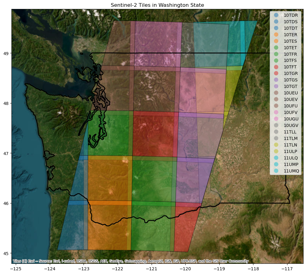
# metadata_gdf.explore("s2:granule_id",
# categorical=True,
# )
3. Loading Sentinel-2 Imagery with odc-stac#
Let’s search the STAC catalog for a smaller area with a longer time range–we’ll focus again on Mt. Rainier throughout July 2024#
import odc.stac
import rioxarray
start_date = "2024-07-01"
end_date = "2024-07-31"
rainier_bbox_gdf = gpd.read_file("https://github.com/egagli/easysnowdata/raw/main/docs/examples/mt_rainier.geojson")
bbox = rainier_bbox_gdf.total_bounds
bbox
array([-121.94224976, 46.72842173, -121.54136001, 46.99728203])
search = catalog.search(
collections=["sentinel-2-l2a"], # sentinel-2-c1-l2a if using earthsearch
bbox=bbox,
datetime=(start_date, end_date),
#query={"eo:cloud_cover": {"lt": 30}},
)
items = search.item_collection()
items
- type "FeatureCollection"
features[] 48 items
0
- type "Feature"
- stac_version "1.1.0"
stac_extensions[] 3 items
- 0 "https://stac-extensions.github.io/eo/v1.1.0/schema.json"
- 1 "https://stac-extensions.github.io/sat/v1.0.0/schema.json"
- 2 "https://stac-extensions.github.io/projection/v2.0.0/schema.json"
- id "S2B_MSIL2A_20240730T185919_R013_T10TFT_20240730T214651"
geometry
- type "Polygon"
coordinates[] 1 items
0[] 5 items
0[] 2 items
- 0 -121.6633998
- 1 47.8459211
1[] 2 items
- 0 -120.1971533
- 1 47.8194744
2[] 2 items
- 0 -120.248915
- 1 46.8326283
3[] 2 items
- 0 -121.6881131
- 1 46.858182
4[] 2 items
- 0 -121.6633998
- 1 47.8459211
bbox[] 4 items
- 0 -121.6881131
- 1 46.8326283
- 2 -120.1971533
- 3 47.8459211
properties
- datetime "2024-07-30T18:59:19.024000Z"
- platform "Sentinel-2B"
instruments[] 1 items
- 0 "msi"
- s2:mgrs_tile "10TFT"
- constellation "Sentinel 2"
- s2:granule_id "S2B_OPER_MSI_L2A_TL_2BPS_20240730T214651_A038649_T10TFT_N05.11"
- eo:cloud_cover 59.944248
- s2:datatake_id "GS2B_20240730T185919_038649_N05.11"
- s2:product_uri "S2B_MSIL2A_20240730T185919_N0511_R013_T10TFT_20240730T214651.SAFE"
- s2:datastrip_id "S2B_OPER_MSI_L2A_DS_2BPS_20240730T214651_S20240730T190733_N05.11"
- s2:product_type "S2MSI2A"
- sat:orbit_state "descending"
- s2:datatake_type "INS-NOBS"
- s2:generation_time "2024-07-30T21:46:51.000000Z"
- sat:relative_orbit 13
- s2:water_percentage 0.274399
- s2:mean_solar_zenith 31.4952476102959
- s2:mean_solar_azimuth 152.527652573228
- s2:processing_baseline "05.11"
- s2:snow_ice_percentage 0.01295
- s2:vegetation_percentage 19.018488
- s2:thin_cirrus_percentage 0.172362
- s2:cloud_shadow_percentage 1.921573
- s2:nodata_pixel_percentage 0.0
- s2:unclassified_percentage 2.879881
- s2:not_vegetated_percentage 14.80495
- s2:degraded_msi_data_percentage 0.0094
- s2:high_proba_clouds_percentage 51.149404
- s2:reflectance_conversion_factor 0.969685193843776
- s2:medium_proba_clouds_percentage 8.622486
- s2:saturated_defective_pixel_percentage 0.0
- proj:code "EPSG:32610"
links[] 6 items
0
- rel "collection"
- href "https://planetarycomputer.microsoft.com/api/stac/v1/collections/sentinel-2-l2a"
- type "application/json"
1
- rel "parent"
- href "https://planetarycomputer.microsoft.com/api/stac/v1/collections/sentinel-2-l2a"
- type "application/json"
2
- rel "root"
- href "https://planetarycomputer.microsoft.com/api/stac/v1"
- type "application/json"
- title "Microsoft Planetary Computer STAC API"
3
- rel "self"
- href "https://planetarycomputer.microsoft.com/api/stac/v1/collections/sentinel-2-l2a/items/S2B_MSIL2A_20240730T185919_R013_T10TFT_20240730T214651"
- type "application/geo+json"
4
- rel "license"
- href "https://sentinel.esa.int/documents/247904/690755/Sentinel_Data_Legal_Notice"
5
- rel "preview"
- href "https://planetarycomputer.microsoft.com/api/data/v1/item/map?collection=sentinel-2-l2a&item=S2B_MSIL2A_20240730T185919_R013_T10TFT_20240730T214651"
- type "text/html"
- title "Map of item"
assets
AOT
- href "https://sentinel2l2a01.blob.core.windows.net/sentinel2-l2/10/T/FT/2024/07/30/S2B_MSIL2A_20240730T185919_N0511_R013_T10TFT_20240730T214651.SAFE/GRANULE/L2A_T10TFT_A038649_20240730T190733/IMG_DATA/R10m/T10TFT_20240730T185919_AOT_10m.tif?st=2025-03-03T03%3A04%3A03Z&se=2025-03-04T03%3A49%3A03Z&sp=rl&sv=2024-05-04&sr=c&skoid=9c8ff44a-6a2c-4dfb-b298-1c9212f64d9a&sktid=72f988bf-86f1-41af-91ab-2d7cd011db47&skt=2025-03-04T01%3A57%3A30Z&ske=2025-03-11T01%3A57%3A30Z&sks=b&skv=2024-05-04&sig=0Ih4Xpb0cU%2B%2BNRJlN354z9Pm1tJS4xxWr5cZWryvGzE%3D"
- type "image/tiff; application=geotiff; profile=cloud-optimized"
- title "Aerosol optical thickness (AOT)"
proj:bbox[] 4 items
- 0 600000.0
- 1 5190240.0
- 2 709800.0
- 3 5300040.0
proj:shape[] 2 items
- 0 10980
- 1 10980
proj:transform[] 6 items
- 0 10.0
- 1 0.0
- 2 600000.0
- 3 0.0
- 4 -10.0
- 5 5300040.0
- gsd 10.0
roles[] 1 items
- 0 "data"
B01
- href "https://sentinel2l2a01.blob.core.windows.net/sentinel2-l2/10/T/FT/2024/07/30/S2B_MSIL2A_20240730T185919_N0511_R013_T10TFT_20240730T214651.SAFE/GRANULE/L2A_T10TFT_A038649_20240730T190733/IMG_DATA/R60m/T10TFT_20240730T185919_B01_60m.tif?st=2025-03-03T03%3A04%3A03Z&se=2025-03-04T03%3A49%3A03Z&sp=rl&sv=2024-05-04&sr=c&skoid=9c8ff44a-6a2c-4dfb-b298-1c9212f64d9a&sktid=72f988bf-86f1-41af-91ab-2d7cd011db47&skt=2025-03-04T01%3A57%3A30Z&ske=2025-03-11T01%3A57%3A30Z&sks=b&skv=2024-05-04&sig=0Ih4Xpb0cU%2B%2BNRJlN354z9Pm1tJS4xxWr5cZWryvGzE%3D"
- type "image/tiff; application=geotiff; profile=cloud-optimized"
- title "Band 1 - Coastal aerosol - 60m"
proj:bbox[] 4 items
- 0 600000.0
- 1 5190240.0
- 2 709800.0
- 3 5300040.0
proj:shape[] 2 items
- 0 1830
- 1 1830
proj:transform[] 6 items
- 0 60.0
- 1 0.0
- 2 600000.0
- 3 0.0
- 4 -60.0
- 5 5300040.0
- gsd 60.0
eo:bands[] 1 items
0
- name "B01"
- common_name "coastal"
- description "Band 1 - Coastal aerosol"
- center_wavelength 0.443
- full_width_half_max 0.027
roles[] 1 items
- 0 "data"
B02
- href "https://sentinel2l2a01.blob.core.windows.net/sentinel2-l2/10/T/FT/2024/07/30/S2B_MSIL2A_20240730T185919_N0511_R013_T10TFT_20240730T214651.SAFE/GRANULE/L2A_T10TFT_A038649_20240730T190733/IMG_DATA/R10m/T10TFT_20240730T185919_B02_10m.tif?st=2025-03-03T03%3A04%3A03Z&se=2025-03-04T03%3A49%3A03Z&sp=rl&sv=2024-05-04&sr=c&skoid=9c8ff44a-6a2c-4dfb-b298-1c9212f64d9a&sktid=72f988bf-86f1-41af-91ab-2d7cd011db47&skt=2025-03-04T01%3A57%3A30Z&ske=2025-03-11T01%3A57%3A30Z&sks=b&skv=2024-05-04&sig=0Ih4Xpb0cU%2B%2BNRJlN354z9Pm1tJS4xxWr5cZWryvGzE%3D"
- type "image/tiff; application=geotiff; profile=cloud-optimized"
- title "Band 2 - Blue - 10m"
proj:bbox[] 4 items
- 0 600000.0
- 1 5190240.0
- 2 709800.0
- 3 5300040.0
proj:shape[] 2 items
- 0 10980
- 1 10980
proj:transform[] 6 items
- 0 10.0
- 1 0.0
- 2 600000.0
- 3 0.0
- 4 -10.0
- 5 5300040.0
- gsd 10.0
eo:bands[] 1 items
0
- name "B02"
- common_name "blue"
- description "Band 2 - Blue"
- center_wavelength 0.49
- full_width_half_max 0.098
roles[] 1 items
- 0 "data"
B03
- href "https://sentinel2l2a01.blob.core.windows.net/sentinel2-l2/10/T/FT/2024/07/30/S2B_MSIL2A_20240730T185919_N0511_R013_T10TFT_20240730T214651.SAFE/GRANULE/L2A_T10TFT_A038649_20240730T190733/IMG_DATA/R10m/T10TFT_20240730T185919_B03_10m.tif?st=2025-03-03T03%3A04%3A03Z&se=2025-03-04T03%3A49%3A03Z&sp=rl&sv=2024-05-04&sr=c&skoid=9c8ff44a-6a2c-4dfb-b298-1c9212f64d9a&sktid=72f988bf-86f1-41af-91ab-2d7cd011db47&skt=2025-03-04T01%3A57%3A30Z&ske=2025-03-11T01%3A57%3A30Z&sks=b&skv=2024-05-04&sig=0Ih4Xpb0cU%2B%2BNRJlN354z9Pm1tJS4xxWr5cZWryvGzE%3D"
- type "image/tiff; application=geotiff; profile=cloud-optimized"
- title "Band 3 - Green - 10m"
proj:bbox[] 4 items
- 0 600000.0
- 1 5190240.0
- 2 709800.0
- 3 5300040.0
proj:shape[] 2 items
- 0 10980
- 1 10980
proj:transform[] 6 items
- 0 10.0
- 1 0.0
- 2 600000.0
- 3 0.0
- 4 -10.0
- 5 5300040.0
- gsd 10.0
eo:bands[] 1 items
0
- name "B03"
- common_name "green"
- description "Band 3 - Green"
- center_wavelength 0.56
- full_width_half_max 0.045
roles[] 1 items
- 0 "data"
B04
- href "https://sentinel2l2a01.blob.core.windows.net/sentinel2-l2/10/T/FT/2024/07/30/S2B_MSIL2A_20240730T185919_N0511_R013_T10TFT_20240730T214651.SAFE/GRANULE/L2A_T10TFT_A038649_20240730T190733/IMG_DATA/R10m/T10TFT_20240730T185919_B04_10m.tif?st=2025-03-03T03%3A04%3A03Z&se=2025-03-04T03%3A49%3A03Z&sp=rl&sv=2024-05-04&sr=c&skoid=9c8ff44a-6a2c-4dfb-b298-1c9212f64d9a&sktid=72f988bf-86f1-41af-91ab-2d7cd011db47&skt=2025-03-04T01%3A57%3A30Z&ske=2025-03-11T01%3A57%3A30Z&sks=b&skv=2024-05-04&sig=0Ih4Xpb0cU%2B%2BNRJlN354z9Pm1tJS4xxWr5cZWryvGzE%3D"
- type "image/tiff; application=geotiff; profile=cloud-optimized"
- title "Band 4 - Red - 10m"
proj:bbox[] 4 items
- 0 600000.0
- 1 5190240.0
- 2 709800.0
- 3 5300040.0
proj:shape[] 2 items
- 0 10980
- 1 10980
proj:transform[] 6 items
- 0 10.0
- 1 0.0
- 2 600000.0
- 3 0.0
- 4 -10.0
- 5 5300040.0
- gsd 10.0
eo:bands[] 1 items
0
- name "B04"
- common_name "red"
- description "Band 4 - Red"
- center_wavelength 0.665
- full_width_half_max 0.038
roles[] 1 items
- 0 "data"
B05
- href "https://sentinel2l2a01.blob.core.windows.net/sentinel2-l2/10/T/FT/2024/07/30/S2B_MSIL2A_20240730T185919_N0511_R013_T10TFT_20240730T214651.SAFE/GRANULE/L2A_T10TFT_A038649_20240730T190733/IMG_DATA/R20m/T10TFT_20240730T185919_B05_20m.tif?st=2025-03-03T03%3A04%3A03Z&se=2025-03-04T03%3A49%3A03Z&sp=rl&sv=2024-05-04&sr=c&skoid=9c8ff44a-6a2c-4dfb-b298-1c9212f64d9a&sktid=72f988bf-86f1-41af-91ab-2d7cd011db47&skt=2025-03-04T01%3A57%3A30Z&ske=2025-03-11T01%3A57%3A30Z&sks=b&skv=2024-05-04&sig=0Ih4Xpb0cU%2B%2BNRJlN354z9Pm1tJS4xxWr5cZWryvGzE%3D"
- type "image/tiff; application=geotiff; profile=cloud-optimized"
- title "Band 5 - Vegetation red edge 1 - 20m"
proj:bbox[] 4 items
- 0 600000.0
- 1 5190240.0
- 2 709800.0
- 3 5300040.0
proj:shape[] 2 items
- 0 5490
- 1 5490
proj:transform[] 6 items
- 0 20.0
- 1 0.0
- 2 600000.0
- 3 0.0
- 4 -20.0
- 5 5300040.0
- gsd 20.0
eo:bands[] 1 items
0
- name "B05"
- common_name "rededge"
- description "Band 5 - Vegetation red edge 1"
- center_wavelength 0.704
- full_width_half_max 0.019
roles[] 1 items
- 0 "data"
B06
- href "https://sentinel2l2a01.blob.core.windows.net/sentinel2-l2/10/T/FT/2024/07/30/S2B_MSIL2A_20240730T185919_N0511_R013_T10TFT_20240730T214651.SAFE/GRANULE/L2A_T10TFT_A038649_20240730T190733/IMG_DATA/R20m/T10TFT_20240730T185919_B06_20m.tif?st=2025-03-03T03%3A04%3A03Z&se=2025-03-04T03%3A49%3A03Z&sp=rl&sv=2024-05-04&sr=c&skoid=9c8ff44a-6a2c-4dfb-b298-1c9212f64d9a&sktid=72f988bf-86f1-41af-91ab-2d7cd011db47&skt=2025-03-04T01%3A57%3A30Z&ske=2025-03-11T01%3A57%3A30Z&sks=b&skv=2024-05-04&sig=0Ih4Xpb0cU%2B%2BNRJlN354z9Pm1tJS4xxWr5cZWryvGzE%3D"
- type "image/tiff; application=geotiff; profile=cloud-optimized"
- title "Band 6 - Vegetation red edge 2 - 20m"
proj:bbox[] 4 items
- 0 600000.0
- 1 5190240.0
- 2 709800.0
- 3 5300040.0
proj:shape[] 2 items
- 0 5490
- 1 5490
proj:transform[] 6 items
- 0 20.0
- 1 0.0
- 2 600000.0
- 3 0.0
- 4 -20.0
- 5 5300040.0
- gsd 20.0
eo:bands[] 1 items
0
- name "B06"
- common_name "rededge"
- description "Band 6 - Vegetation red edge 2"
- center_wavelength 0.74
- full_width_half_max 0.018
roles[] 1 items
- 0 "data"
B07
- href "https://sentinel2l2a01.blob.core.windows.net/sentinel2-l2/10/T/FT/2024/07/30/S2B_MSIL2A_20240730T185919_N0511_R013_T10TFT_20240730T214651.SAFE/GRANULE/L2A_T10TFT_A038649_20240730T190733/IMG_DATA/R20m/T10TFT_20240730T185919_B07_20m.tif?st=2025-03-03T03%3A04%3A03Z&se=2025-03-04T03%3A49%3A03Z&sp=rl&sv=2024-05-04&sr=c&skoid=9c8ff44a-6a2c-4dfb-b298-1c9212f64d9a&sktid=72f988bf-86f1-41af-91ab-2d7cd011db47&skt=2025-03-04T01%3A57%3A30Z&ske=2025-03-11T01%3A57%3A30Z&sks=b&skv=2024-05-04&sig=0Ih4Xpb0cU%2B%2BNRJlN354z9Pm1tJS4xxWr5cZWryvGzE%3D"
- type "image/tiff; application=geotiff; profile=cloud-optimized"
- title "Band 7 - Vegetation red edge 3 - 20m"
proj:bbox[] 4 items
- 0 600000.0
- 1 5190240.0
- 2 709800.0
- 3 5300040.0
proj:shape[] 2 items
- 0 5490
- 1 5490
proj:transform[] 6 items
- 0 20.0
- 1 0.0
- 2 600000.0
- 3 0.0
- 4 -20.0
- 5 5300040.0
- gsd 20.0
eo:bands[] 1 items
0
- name "B07"
- common_name "rededge"
- description "Band 7 - Vegetation red edge 3"
- center_wavelength 0.783
- full_width_half_max 0.028
roles[] 1 items
- 0 "data"
B08
- href "https://sentinel2l2a01.blob.core.windows.net/sentinel2-l2/10/T/FT/2024/07/30/S2B_MSIL2A_20240730T185919_N0511_R013_T10TFT_20240730T214651.SAFE/GRANULE/L2A_T10TFT_A038649_20240730T190733/IMG_DATA/R10m/T10TFT_20240730T185919_B08_10m.tif?st=2025-03-03T03%3A04%3A03Z&se=2025-03-04T03%3A49%3A03Z&sp=rl&sv=2024-05-04&sr=c&skoid=9c8ff44a-6a2c-4dfb-b298-1c9212f64d9a&sktid=72f988bf-86f1-41af-91ab-2d7cd011db47&skt=2025-03-04T01%3A57%3A30Z&ske=2025-03-11T01%3A57%3A30Z&sks=b&skv=2024-05-04&sig=0Ih4Xpb0cU%2B%2BNRJlN354z9Pm1tJS4xxWr5cZWryvGzE%3D"
- type "image/tiff; application=geotiff; profile=cloud-optimized"
- title "Band 8 - NIR - 10m"
proj:bbox[] 4 items
- 0 600000.0
- 1 5190240.0
- 2 709800.0
- 3 5300040.0
proj:shape[] 2 items
- 0 10980
- 1 10980
proj:transform[] 6 items
- 0 10.0
- 1 0.0
- 2 600000.0
- 3 0.0
- 4 -10.0
- 5 5300040.0
- gsd 10.0
eo:bands[] 1 items
0
- name "B08"
- common_name "nir"
- description "Band 8 - NIR"
- center_wavelength 0.842
- full_width_half_max 0.145
roles[] 1 items
- 0 "data"
B09
- href "https://sentinel2l2a01.blob.core.windows.net/sentinel2-l2/10/T/FT/2024/07/30/S2B_MSIL2A_20240730T185919_N0511_R013_T10TFT_20240730T214651.SAFE/GRANULE/L2A_T10TFT_A038649_20240730T190733/IMG_DATA/R60m/T10TFT_20240730T185919_B09_60m.tif?st=2025-03-03T03%3A04%3A03Z&se=2025-03-04T03%3A49%3A03Z&sp=rl&sv=2024-05-04&sr=c&skoid=9c8ff44a-6a2c-4dfb-b298-1c9212f64d9a&sktid=72f988bf-86f1-41af-91ab-2d7cd011db47&skt=2025-03-04T01%3A57%3A30Z&ske=2025-03-11T01%3A57%3A30Z&sks=b&skv=2024-05-04&sig=0Ih4Xpb0cU%2B%2BNRJlN354z9Pm1tJS4xxWr5cZWryvGzE%3D"
- type "image/tiff; application=geotiff; profile=cloud-optimized"
- title "Band 9 - Water vapor - 60m"
proj:bbox[] 4 items
- 0 600000.0
- 1 5190240.0
- 2 709800.0
- 3 5300040.0
proj:shape[] 2 items
- 0 1830
- 1 1830
proj:transform[] 6 items
- 0 60.0
- 1 0.0
- 2 600000.0
- 3 0.0
- 4 -60.0
- 5 5300040.0
- gsd 60.0
eo:bands[] 1 items
0
- name "B09"
- description "Band 9 - Water vapor"
- center_wavelength 0.945
- full_width_half_max 0.026
roles[] 1 items
- 0 "data"
B11
- href "https://sentinel2l2a01.blob.core.windows.net/sentinel2-l2/10/T/FT/2024/07/30/S2B_MSIL2A_20240730T185919_N0511_R013_T10TFT_20240730T214651.SAFE/GRANULE/L2A_T10TFT_A038649_20240730T190733/IMG_DATA/R20m/T10TFT_20240730T185919_B11_20m.tif?st=2025-03-03T03%3A04%3A03Z&se=2025-03-04T03%3A49%3A03Z&sp=rl&sv=2024-05-04&sr=c&skoid=9c8ff44a-6a2c-4dfb-b298-1c9212f64d9a&sktid=72f988bf-86f1-41af-91ab-2d7cd011db47&skt=2025-03-04T01%3A57%3A30Z&ske=2025-03-11T01%3A57%3A30Z&sks=b&skv=2024-05-04&sig=0Ih4Xpb0cU%2B%2BNRJlN354z9Pm1tJS4xxWr5cZWryvGzE%3D"
- type "image/tiff; application=geotiff; profile=cloud-optimized"
- title "Band 11 - SWIR (1.6) - 20m"
proj:bbox[] 4 items
- 0 600000.0
- 1 5190240.0
- 2 709800.0
- 3 5300040.0
proj:shape[] 2 items
- 0 5490
- 1 5490
proj:transform[] 6 items
- 0 20.0
- 1 0.0
- 2 600000.0
- 3 0.0
- 4 -20.0
- 5 5300040.0
- gsd 20.0
eo:bands[] 1 items
0
- name "B11"
- common_name "swir16"
- description "Band 11 - SWIR (1.6)"
- center_wavelength 1.61
- full_width_half_max 0.143
roles[] 1 items
- 0 "data"
B12
- href "https://sentinel2l2a01.blob.core.windows.net/sentinel2-l2/10/T/FT/2024/07/30/S2B_MSIL2A_20240730T185919_N0511_R013_T10TFT_20240730T214651.SAFE/GRANULE/L2A_T10TFT_A038649_20240730T190733/IMG_DATA/R20m/T10TFT_20240730T185919_B12_20m.tif?st=2025-03-03T03%3A04%3A03Z&se=2025-03-04T03%3A49%3A03Z&sp=rl&sv=2024-05-04&sr=c&skoid=9c8ff44a-6a2c-4dfb-b298-1c9212f64d9a&sktid=72f988bf-86f1-41af-91ab-2d7cd011db47&skt=2025-03-04T01%3A57%3A30Z&ske=2025-03-11T01%3A57%3A30Z&sks=b&skv=2024-05-04&sig=0Ih4Xpb0cU%2B%2BNRJlN354z9Pm1tJS4xxWr5cZWryvGzE%3D"
- type "image/tiff; application=geotiff; profile=cloud-optimized"
- title "Band 12 - SWIR (2.2) - 20m"
proj:bbox[] 4 items
- 0 600000.0
- 1 5190240.0
- 2 709800.0
- 3 5300040.0
proj:shape[] 2 items
- 0 5490
- 1 5490
proj:transform[] 6 items
- 0 20.0
- 1 0.0
- 2 600000.0
- 3 0.0
- 4 -20.0
- 5 5300040.0
- gsd 20.0
eo:bands[] 1 items
0
- name "B12"
- common_name "swir22"
- description "Band 12 - SWIR (2.2)"
- center_wavelength 2.19
- full_width_half_max 0.242
roles[] 1 items
- 0 "data"
B8A
- href "https://sentinel2l2a01.blob.core.windows.net/sentinel2-l2/10/T/FT/2024/07/30/S2B_MSIL2A_20240730T185919_N0511_R013_T10TFT_20240730T214651.SAFE/GRANULE/L2A_T10TFT_A038649_20240730T190733/IMG_DATA/R20m/T10TFT_20240730T185919_B8A_20m.tif?st=2025-03-03T03%3A04%3A03Z&se=2025-03-04T03%3A49%3A03Z&sp=rl&sv=2024-05-04&sr=c&skoid=9c8ff44a-6a2c-4dfb-b298-1c9212f64d9a&sktid=72f988bf-86f1-41af-91ab-2d7cd011db47&skt=2025-03-04T01%3A57%3A30Z&ske=2025-03-11T01%3A57%3A30Z&sks=b&skv=2024-05-04&sig=0Ih4Xpb0cU%2B%2BNRJlN354z9Pm1tJS4xxWr5cZWryvGzE%3D"
- type "image/tiff; application=geotiff; profile=cloud-optimized"
- title "Band 8A - Vegetation red edge 4 - 20m"
proj:bbox[] 4 items
- 0 600000.0
- 1 5190240.0
- 2 709800.0
- 3 5300040.0
proj:shape[] 2 items
- 0 5490
- 1 5490
proj:transform[] 6 items
- 0 20.0
- 1 0.0
- 2 600000.0
- 3 0.0
- 4 -20.0
- 5 5300040.0
- gsd 20.0
eo:bands[] 1 items
0
- name "B8A"
- common_name "rededge"
- description "Band 8A - Vegetation red edge 4"
- center_wavelength 0.865
- full_width_half_max 0.033
roles[] 1 items
- 0 "data"
SCL
- href "https://sentinel2l2a01.blob.core.windows.net/sentinel2-l2/10/T/FT/2024/07/30/S2B_MSIL2A_20240730T185919_N0511_R013_T10TFT_20240730T214651.SAFE/GRANULE/L2A_T10TFT_A038649_20240730T190733/IMG_DATA/R20m/T10TFT_20240730T185919_SCL_20m.tif?st=2025-03-03T03%3A04%3A03Z&se=2025-03-04T03%3A49%3A03Z&sp=rl&sv=2024-05-04&sr=c&skoid=9c8ff44a-6a2c-4dfb-b298-1c9212f64d9a&sktid=72f988bf-86f1-41af-91ab-2d7cd011db47&skt=2025-03-04T01%3A57%3A30Z&ske=2025-03-11T01%3A57%3A30Z&sks=b&skv=2024-05-04&sig=0Ih4Xpb0cU%2B%2BNRJlN354z9Pm1tJS4xxWr5cZWryvGzE%3D"
- type "image/tiff; application=geotiff; profile=cloud-optimized"
- title "Scene classfication map (SCL)"
proj:bbox[] 4 items
- 0 600000.0
- 1 5190240.0
- 2 709800.0
- 3 5300040.0
proj:shape[] 2 items
- 0 5490
- 1 5490
proj:transform[] 6 items
- 0 20.0
- 1 0.0
- 2 600000.0
- 3 0.0
- 4 -20.0
- 5 5300040.0
- gsd 20.0
roles[] 1 items
- 0 "data"
WVP
- href "https://sentinel2l2a01.blob.core.windows.net/sentinel2-l2/10/T/FT/2024/07/30/S2B_MSIL2A_20240730T185919_N0511_R013_T10TFT_20240730T214651.SAFE/GRANULE/L2A_T10TFT_A038649_20240730T190733/IMG_DATA/R10m/T10TFT_20240730T185919_WVP_10m.tif?st=2025-03-03T03%3A04%3A03Z&se=2025-03-04T03%3A49%3A03Z&sp=rl&sv=2024-05-04&sr=c&skoid=9c8ff44a-6a2c-4dfb-b298-1c9212f64d9a&sktid=72f988bf-86f1-41af-91ab-2d7cd011db47&skt=2025-03-04T01%3A57%3A30Z&ske=2025-03-11T01%3A57%3A30Z&sks=b&skv=2024-05-04&sig=0Ih4Xpb0cU%2B%2BNRJlN354z9Pm1tJS4xxWr5cZWryvGzE%3D"
- type "image/tiff; application=geotiff; profile=cloud-optimized"
- title "Water vapour (WVP)"
proj:bbox[] 4 items
- 0 600000.0
- 1 5190240.0
- 2 709800.0
- 3 5300040.0
proj:shape[] 2 items
- 0 10980
- 1 10980
proj:transform[] 6 items
- 0 10.0
- 1 0.0
- 2 600000.0
- 3 0.0
- 4 -10.0
- 5 5300040.0
- gsd 10.0
roles[] 1 items
- 0 "data"
visual
- href "https://sentinel2l2a01.blob.core.windows.net/sentinel2-l2/10/T/FT/2024/07/30/S2B_MSIL2A_20240730T185919_N0511_R013_T10TFT_20240730T214651.SAFE/GRANULE/L2A_T10TFT_A038649_20240730T190733/IMG_DATA/R10m/T10TFT_20240730T185919_TCI_10m.tif?st=2025-03-03T03%3A04%3A03Z&se=2025-03-04T03%3A49%3A03Z&sp=rl&sv=2024-05-04&sr=c&skoid=9c8ff44a-6a2c-4dfb-b298-1c9212f64d9a&sktid=72f988bf-86f1-41af-91ab-2d7cd011db47&skt=2025-03-04T01%3A57%3A30Z&ske=2025-03-11T01%3A57%3A30Z&sks=b&skv=2024-05-04&sig=0Ih4Xpb0cU%2B%2BNRJlN354z9Pm1tJS4xxWr5cZWryvGzE%3D"
- type "image/tiff; application=geotiff; profile=cloud-optimized"
- title "True color image"
proj:bbox[] 4 items
- 0 600000.0
- 1 5190240.0
- 2 709800.0
- 3 5300040.0
proj:shape[] 2 items
- 0 10980
- 1 10980
proj:transform[] 6 items
- 0 10.0
- 1 0.0
- 2 600000.0
- 3 0.0
- 4 -10.0
- 5 5300040.0
- gsd 10.0
eo:bands[] 3 items
0
- name "B04"
- common_name "red"
- description "Band 4 - Red"
- center_wavelength 0.665
- full_width_half_max 0.038
1
- name "B03"
- common_name "green"
- description "Band 3 - Green"
- center_wavelength 0.56
- full_width_half_max 0.045
2
- name "B02"
- common_name "blue"
- description "Band 2 - Blue"
- center_wavelength 0.49
- full_width_half_max 0.098
roles[] 1 items
- 0 "data"
safe-manifest
- href "https://sentinel2l2a01.blob.core.windows.net/sentinel2-l2/10/T/FT/2024/07/30/S2B_MSIL2A_20240730T185919_N0511_R013_T10TFT_20240730T214651.SAFE/manifest.safe?st=2025-03-03T03%3A04%3A03Z&se=2025-03-04T03%3A49%3A03Z&sp=rl&sv=2024-05-04&sr=c&skoid=9c8ff44a-6a2c-4dfb-b298-1c9212f64d9a&sktid=72f988bf-86f1-41af-91ab-2d7cd011db47&skt=2025-03-04T01%3A57%3A30Z&ske=2025-03-11T01%3A57%3A30Z&sks=b&skv=2024-05-04&sig=0Ih4Xpb0cU%2B%2BNRJlN354z9Pm1tJS4xxWr5cZWryvGzE%3D"
- type "application/xml"
- title "SAFE manifest"
roles[] 1 items
- 0 "metadata"
granule-metadata
- href "https://sentinel2l2a01.blob.core.windows.net/sentinel2-l2/10/T/FT/2024/07/30/S2B_MSIL2A_20240730T185919_N0511_R013_T10TFT_20240730T214651.SAFE/GRANULE/L2A_T10TFT_A038649_20240730T190733/MTD_TL.xml?st=2025-03-03T03%3A04%3A03Z&se=2025-03-04T03%3A49%3A03Z&sp=rl&sv=2024-05-04&sr=c&skoid=9c8ff44a-6a2c-4dfb-b298-1c9212f64d9a&sktid=72f988bf-86f1-41af-91ab-2d7cd011db47&skt=2025-03-04T01%3A57%3A30Z&ske=2025-03-11T01%3A57%3A30Z&sks=b&skv=2024-05-04&sig=0Ih4Xpb0cU%2B%2BNRJlN354z9Pm1tJS4xxWr5cZWryvGzE%3D"
- type "application/xml"
- title "Granule metadata"
roles[] 1 items
- 0 "metadata"
inspire-metadata
- href "https://sentinel2l2a01.blob.core.windows.net/sentinel2-l2/10/T/FT/2024/07/30/S2B_MSIL2A_20240730T185919_N0511_R013_T10TFT_20240730T214651.SAFE/INSPIRE.xml?st=2025-03-03T03%3A04%3A03Z&se=2025-03-04T03%3A49%3A03Z&sp=rl&sv=2024-05-04&sr=c&skoid=9c8ff44a-6a2c-4dfb-b298-1c9212f64d9a&sktid=72f988bf-86f1-41af-91ab-2d7cd011db47&skt=2025-03-04T01%3A57%3A30Z&ske=2025-03-11T01%3A57%3A30Z&sks=b&skv=2024-05-04&sig=0Ih4Xpb0cU%2B%2BNRJlN354z9Pm1tJS4xxWr5cZWryvGzE%3D"
- type "application/xml"
- title "INSPIRE metadata"
roles[] 1 items
- 0 "metadata"
product-metadata
- href "https://sentinel2l2a01.blob.core.windows.net/sentinel2-l2/10/T/FT/2024/07/30/S2B_MSIL2A_20240730T185919_N0511_R013_T10TFT_20240730T214651.SAFE/MTD_MSIL2A.xml?st=2025-03-03T03%3A04%3A03Z&se=2025-03-04T03%3A49%3A03Z&sp=rl&sv=2024-05-04&sr=c&skoid=9c8ff44a-6a2c-4dfb-b298-1c9212f64d9a&sktid=72f988bf-86f1-41af-91ab-2d7cd011db47&skt=2025-03-04T01%3A57%3A30Z&ske=2025-03-11T01%3A57%3A30Z&sks=b&skv=2024-05-04&sig=0Ih4Xpb0cU%2B%2BNRJlN354z9Pm1tJS4xxWr5cZWryvGzE%3D"
- type "application/xml"
- title "Product metadata"
roles[] 1 items
- 0 "metadata"
datastrip-metadata
- href "https://sentinel2l2a01.blob.core.windows.net/sentinel2-l2/10/T/FT/2024/07/30/S2B_MSIL2A_20240730T185919_N0511_R013_T10TFT_20240730T214651.SAFE/DATASTRIP/DS_2BPS_20240730T214651_S20240730T190733/MTD_DS.xml?st=2025-03-03T03%3A04%3A03Z&se=2025-03-04T03%3A49%3A03Z&sp=rl&sv=2024-05-04&sr=c&skoid=9c8ff44a-6a2c-4dfb-b298-1c9212f64d9a&sktid=72f988bf-86f1-41af-91ab-2d7cd011db47&skt=2025-03-04T01%3A57%3A30Z&ske=2025-03-11T01%3A57%3A30Z&sks=b&skv=2024-05-04&sig=0Ih4Xpb0cU%2B%2BNRJlN354z9Pm1tJS4xxWr5cZWryvGzE%3D"
- type "application/xml"
- title "Datastrip metadata"
roles[] 1 items
- 0 "metadata"
tilejson
- href "https://planetarycomputer.microsoft.com/api/data/v1/item/tilejson.json?collection=sentinel-2-l2a&item=S2B_MSIL2A_20240730T185919_R013_T10TFT_20240730T214651&assets=visual&asset_bidx=visual%7C1%2C2%2C3&nodata=0&format=png"
- type "application/json"
- title "TileJSON with default rendering"
roles[] 1 items
- 0 "tiles"
rendered_preview
- href "https://planetarycomputer.microsoft.com/api/data/v1/item/preview.png?collection=sentinel-2-l2a&item=S2B_MSIL2A_20240730T185919_R013_T10TFT_20240730T214651&assets=visual&asset_bidx=visual%7C1%2C2%2C3&nodata=0&format=png"
- type "image/png"
- title "Rendered preview"
- rel "preview"
roles[] 1 items
- 0 "overview"
- collection "sentinel-2-l2a"
1
- type "Feature"
- stac_version "1.1.0"
stac_extensions[] 3 items
- 0 "https://stac-extensions.github.io/eo/v1.1.0/schema.json"
- 1 "https://stac-extensions.github.io/sat/v1.0.0/schema.json"
- 2 "https://stac-extensions.github.io/projection/v2.0.0/schema.json"
- id "S2B_MSIL2A_20240730T185919_R013_T10TFS_20240730T214651"
geometry
- type "Polygon"
coordinates[] 1 items
0[] 5 items
0[] 2 items
- 0 -121.6859647
- 1 46.9461683
1[] 2 items
- 0 -120.2444151
- 1 46.9205364
2[] 2 items
- 0 -120.2937457
- 1 45.9334965
3[] 2 items
- 0 -121.7095159
- 1 45.9582645
4[] 2 items
- 0 -121.6859647
- 1 46.9461683
bbox[] 4 items
- 0 -121.7095159
- 1 45.9334965
- 2 -120.2444151
- 3 46.9461683
properties
- datetime "2024-07-30T18:59:19.024000Z"
- platform "Sentinel-2B"
instruments[] 1 items
- 0 "msi"
- s2:mgrs_tile "10TFS"
- constellation "Sentinel 2"
- s2:granule_id "S2B_OPER_MSI_L2A_TL_2BPS_20240730T214651_A038649_T10TFS_N05.11"
- eo:cloud_cover 46.055353
- s2:datatake_id "GS2B_20240730T185919_038649_N05.11"
- s2:product_uri "S2B_MSIL2A_20240730T185919_N0511_R013_T10TFS_20240730T214651.SAFE"
- s2:datastrip_id "S2B_OPER_MSI_L2A_DS_2BPS_20240730T214651_S20240730T190733_N05.11"
- s2:product_type "S2MSI2A"
- sat:orbit_state "descending"
- s2:datatake_type "INS-NOBS"
- s2:generation_time "2024-07-30T21:46:51.000000Z"
- sat:relative_orbit 13
- s2:water_percentage 0.120713
- s2:mean_solar_zenith 30.6909882283606
- s2:mean_solar_azimuth 151.878695210274
- s2:processing_baseline "05.11"
- s2:snow_ice_percentage 0.249488
- s2:vegetation_percentage 22.66082
- s2:thin_cirrus_percentage 0.251545
- s2:cloud_shadow_percentage 3.25194
- s2:nodata_pixel_percentage 0.0
- s2:unclassified_percentage 3.119034
- s2:not_vegetated_percentage 23.315713
- s2:degraded_msi_data_percentage 0.0027
- s2:high_proba_clouds_percentage 34.820446
- s2:reflectance_conversion_factor 0.969685193843776
- s2:medium_proba_clouds_percentage 10.983361
- s2:saturated_defective_pixel_percentage 0.0
- proj:code "EPSG:32610"
links[] 6 items
0
- rel "collection"
- href "https://planetarycomputer.microsoft.com/api/stac/v1/collections/sentinel-2-l2a"
- type "application/json"
1
- rel "parent"
- href "https://planetarycomputer.microsoft.com/api/stac/v1/collections/sentinel-2-l2a"
- type "application/json"
2
- rel "root"
- href "https://planetarycomputer.microsoft.com/api/stac/v1"
- type "application/json"
- title "Microsoft Planetary Computer STAC API"
3
- rel "self"
- href "https://planetarycomputer.microsoft.com/api/stac/v1/collections/sentinel-2-l2a/items/S2B_MSIL2A_20240730T185919_R013_T10TFS_20240730T214651"
- type "application/geo+json"
4
- rel "license"
- href "https://sentinel.esa.int/documents/247904/690755/Sentinel_Data_Legal_Notice"
5
- rel "preview"
- href "https://planetarycomputer.microsoft.com/api/data/v1/item/map?collection=sentinel-2-l2a&item=S2B_MSIL2A_20240730T185919_R013_T10TFS_20240730T214651"
- type "text/html"
- title "Map of item"
assets
AOT
- href "https://sentinel2l2a01.blob.core.windows.net/sentinel2-l2/10/T/FS/2024/07/30/S2B_MSIL2A_20240730T185919_N0511_R013_T10TFS_20240730T214651.SAFE/GRANULE/L2A_T10TFS_A038649_20240730T190733/IMG_DATA/R10m/T10TFS_20240730T185919_AOT_10m.tif?st=2025-03-03T03%3A04%3A03Z&se=2025-03-04T03%3A49%3A03Z&sp=rl&sv=2024-05-04&sr=c&skoid=9c8ff44a-6a2c-4dfb-b298-1c9212f64d9a&sktid=72f988bf-86f1-41af-91ab-2d7cd011db47&skt=2025-03-04T01%3A57%3A30Z&ske=2025-03-11T01%3A57%3A30Z&sks=b&skv=2024-05-04&sig=0Ih4Xpb0cU%2B%2BNRJlN354z9Pm1tJS4xxWr5cZWryvGzE%3D"
- type "image/tiff; application=geotiff; profile=cloud-optimized"
- title "Aerosol optical thickness (AOT)"
proj:bbox[] 4 items
- 0 600000.0
- 1 5090220.0
- 2 709800.0
- 3 5200020.0
proj:shape[] 2 items
- 0 10980
- 1 10980
proj:transform[] 6 items
- 0 10.0
- 1 0.0
- 2 600000.0
- 3 0.0
- 4 -10.0
- 5 5200020.0
- gsd 10.0
roles[] 1 items
- 0 "data"
B01
- href "https://sentinel2l2a01.blob.core.windows.net/sentinel2-l2/10/T/FS/2024/07/30/S2B_MSIL2A_20240730T185919_N0511_R013_T10TFS_20240730T214651.SAFE/GRANULE/L2A_T10TFS_A038649_20240730T190733/IMG_DATA/R60m/T10TFS_20240730T185919_B01_60m.tif?st=2025-03-03T03%3A04%3A03Z&se=2025-03-04T03%3A49%3A03Z&sp=rl&sv=2024-05-04&sr=c&skoid=9c8ff44a-6a2c-4dfb-b298-1c9212f64d9a&sktid=72f988bf-86f1-41af-91ab-2d7cd011db47&skt=2025-03-04T01%3A57%3A30Z&ske=2025-03-11T01%3A57%3A30Z&sks=b&skv=2024-05-04&sig=0Ih4Xpb0cU%2B%2BNRJlN354z9Pm1tJS4xxWr5cZWryvGzE%3D"
- type "image/tiff; application=geotiff; profile=cloud-optimized"
- title "Band 1 - Coastal aerosol - 60m"
proj:bbox[] 4 items
- 0 600000.0
- 1 5090220.0
- 2 709800.0
- 3 5200020.0
proj:shape[] 2 items
- 0 1830
- 1 1830
proj:transform[] 6 items
- 0 60.0
- 1 0.0
- 2 600000.0
- 3 0.0
- 4 -60.0
- 5 5200020.0
- gsd 60.0
eo:bands[] 1 items
0
- name "B01"
- common_name "coastal"
- description "Band 1 - Coastal aerosol"
- center_wavelength 0.443
- full_width_half_max 0.027
roles[] 1 items
- 0 "data"
B02
- href "https://sentinel2l2a01.blob.core.windows.net/sentinel2-l2/10/T/FS/2024/07/30/S2B_MSIL2A_20240730T185919_N0511_R013_T10TFS_20240730T214651.SAFE/GRANULE/L2A_T10TFS_A038649_20240730T190733/IMG_DATA/R10m/T10TFS_20240730T185919_B02_10m.tif?st=2025-03-03T03%3A04%3A03Z&se=2025-03-04T03%3A49%3A03Z&sp=rl&sv=2024-05-04&sr=c&skoid=9c8ff44a-6a2c-4dfb-b298-1c9212f64d9a&sktid=72f988bf-86f1-41af-91ab-2d7cd011db47&skt=2025-03-04T01%3A57%3A30Z&ske=2025-03-11T01%3A57%3A30Z&sks=b&skv=2024-05-04&sig=0Ih4Xpb0cU%2B%2BNRJlN354z9Pm1tJS4xxWr5cZWryvGzE%3D"
- type "image/tiff; application=geotiff; profile=cloud-optimized"
- title "Band 2 - Blue - 10m"
proj:bbox[] 4 items
- 0 600000.0
- 1 5090220.0
- 2 709800.0
- 3 5200020.0
proj:shape[] 2 items
- 0 10980
- 1 10980
proj:transform[] 6 items
- 0 10.0
- 1 0.0
- 2 600000.0
- 3 0.0
- 4 -10.0
- 5 5200020.0
- gsd 10.0
eo:bands[] 1 items
0
- name "B02"
- common_name "blue"
- description "Band 2 - Blue"
- center_wavelength 0.49
- full_width_half_max 0.098
roles[] 1 items
- 0 "data"
B03
- href "https://sentinel2l2a01.blob.core.windows.net/sentinel2-l2/10/T/FS/2024/07/30/S2B_MSIL2A_20240730T185919_N0511_R013_T10TFS_20240730T214651.SAFE/GRANULE/L2A_T10TFS_A038649_20240730T190733/IMG_DATA/R10m/T10TFS_20240730T185919_B03_10m.tif?st=2025-03-03T03%3A04%3A03Z&se=2025-03-04T03%3A49%3A03Z&sp=rl&sv=2024-05-04&sr=c&skoid=9c8ff44a-6a2c-4dfb-b298-1c9212f64d9a&sktid=72f988bf-86f1-41af-91ab-2d7cd011db47&skt=2025-03-04T01%3A57%3A30Z&ske=2025-03-11T01%3A57%3A30Z&sks=b&skv=2024-05-04&sig=0Ih4Xpb0cU%2B%2BNRJlN354z9Pm1tJS4xxWr5cZWryvGzE%3D"
- type "image/tiff; application=geotiff; profile=cloud-optimized"
- title "Band 3 - Green - 10m"
proj:bbox[] 4 items
- 0 600000.0
- 1 5090220.0
- 2 709800.0
- 3 5200020.0
proj:shape[] 2 items
- 0 10980
- 1 10980
proj:transform[] 6 items
- 0 10.0
- 1 0.0
- 2 600000.0
- 3 0.0
- 4 -10.0
- 5 5200020.0
- gsd 10.0
eo:bands[] 1 items
0
- name "B03"
- common_name "green"
- description "Band 3 - Green"
- center_wavelength 0.56
- full_width_half_max 0.045
roles[] 1 items
- 0 "data"
B04
- href "https://sentinel2l2a01.blob.core.windows.net/sentinel2-l2/10/T/FS/2024/07/30/S2B_MSIL2A_20240730T185919_N0511_R013_T10TFS_20240730T214651.SAFE/GRANULE/L2A_T10TFS_A038649_20240730T190733/IMG_DATA/R10m/T10TFS_20240730T185919_B04_10m.tif?st=2025-03-03T03%3A04%3A03Z&se=2025-03-04T03%3A49%3A03Z&sp=rl&sv=2024-05-04&sr=c&skoid=9c8ff44a-6a2c-4dfb-b298-1c9212f64d9a&sktid=72f988bf-86f1-41af-91ab-2d7cd011db47&skt=2025-03-04T01%3A57%3A30Z&ske=2025-03-11T01%3A57%3A30Z&sks=b&skv=2024-05-04&sig=0Ih4Xpb0cU%2B%2BNRJlN354z9Pm1tJS4xxWr5cZWryvGzE%3D"
- type "image/tiff; application=geotiff; profile=cloud-optimized"
- title "Band 4 - Red - 10m"
proj:bbox[] 4 items
- 0 600000.0
- 1 5090220.0
- 2 709800.0
- 3 5200020.0
proj:shape[] 2 items
- 0 10980
- 1 10980
proj:transform[] 6 items
- 0 10.0
- 1 0.0
- 2 600000.0
- 3 0.0
- 4 -10.0
- 5 5200020.0
- gsd 10.0
eo:bands[] 1 items
0
- name "B04"
- common_name "red"
- description "Band 4 - Red"
- center_wavelength 0.665
- full_width_half_max 0.038
roles[] 1 items
- 0 "data"
B05
- href "https://sentinel2l2a01.blob.core.windows.net/sentinel2-l2/10/T/FS/2024/07/30/S2B_MSIL2A_20240730T185919_N0511_R013_T10TFS_20240730T214651.SAFE/GRANULE/L2A_T10TFS_A038649_20240730T190733/IMG_DATA/R20m/T10TFS_20240730T185919_B05_20m.tif?st=2025-03-03T03%3A04%3A03Z&se=2025-03-04T03%3A49%3A03Z&sp=rl&sv=2024-05-04&sr=c&skoid=9c8ff44a-6a2c-4dfb-b298-1c9212f64d9a&sktid=72f988bf-86f1-41af-91ab-2d7cd011db47&skt=2025-03-04T01%3A57%3A30Z&ske=2025-03-11T01%3A57%3A30Z&sks=b&skv=2024-05-04&sig=0Ih4Xpb0cU%2B%2BNRJlN354z9Pm1tJS4xxWr5cZWryvGzE%3D"
- type "image/tiff; application=geotiff; profile=cloud-optimized"
- title "Band 5 - Vegetation red edge 1 - 20m"
proj:bbox[] 4 items
- 0 600000.0
- 1 5090220.0
- 2 709800.0
- 3 5200020.0
proj:shape[] 2 items
- 0 5490
- 1 5490
proj:transform[] 6 items
- 0 20.0
- 1 0.0
- 2 600000.0
- 3 0.0
- 4 -20.0
- 5 5200020.0
- gsd 20.0
eo:bands[] 1 items
0
- name "B05"
- common_name "rededge"
- description "Band 5 - Vegetation red edge 1"
- center_wavelength 0.704
- full_width_half_max 0.019
roles[] 1 items
- 0 "data"
B06
- href "https://sentinel2l2a01.blob.core.windows.net/sentinel2-l2/10/T/FS/2024/07/30/S2B_MSIL2A_20240730T185919_N0511_R013_T10TFS_20240730T214651.SAFE/GRANULE/L2A_T10TFS_A038649_20240730T190733/IMG_DATA/R20m/T10TFS_20240730T185919_B06_20m.tif?st=2025-03-03T03%3A04%3A03Z&se=2025-03-04T03%3A49%3A03Z&sp=rl&sv=2024-05-04&sr=c&skoid=9c8ff44a-6a2c-4dfb-b298-1c9212f64d9a&sktid=72f988bf-86f1-41af-91ab-2d7cd011db47&skt=2025-03-04T01%3A57%3A30Z&ske=2025-03-11T01%3A57%3A30Z&sks=b&skv=2024-05-04&sig=0Ih4Xpb0cU%2B%2BNRJlN354z9Pm1tJS4xxWr5cZWryvGzE%3D"
- type "image/tiff; application=geotiff; profile=cloud-optimized"
- title "Band 6 - Vegetation red edge 2 - 20m"
proj:bbox[] 4 items
- 0 600000.0
- 1 5090220.0
- 2 709800.0
- 3 5200020.0
proj:shape[] 2 items
- 0 5490
- 1 5490
proj:transform[] 6 items
- 0 20.0
- 1 0.0
- 2 600000.0
- 3 0.0
- 4 -20.0
- 5 5200020.0
- gsd 20.0
eo:bands[] 1 items
0
- name "B06"
- common_name "rededge"
- description "Band 6 - Vegetation red edge 2"
- center_wavelength 0.74
- full_width_half_max 0.018
roles[] 1 items
- 0 "data"
B07
- href "https://sentinel2l2a01.blob.core.windows.net/sentinel2-l2/10/T/FS/2024/07/30/S2B_MSIL2A_20240730T185919_N0511_R013_T10TFS_20240730T214651.SAFE/GRANULE/L2A_T10TFS_A038649_20240730T190733/IMG_DATA/R20m/T10TFS_20240730T185919_B07_20m.tif?st=2025-03-03T03%3A04%3A03Z&se=2025-03-04T03%3A49%3A03Z&sp=rl&sv=2024-05-04&sr=c&skoid=9c8ff44a-6a2c-4dfb-b298-1c9212f64d9a&sktid=72f988bf-86f1-41af-91ab-2d7cd011db47&skt=2025-03-04T01%3A57%3A30Z&ske=2025-03-11T01%3A57%3A30Z&sks=b&skv=2024-05-04&sig=0Ih4Xpb0cU%2B%2BNRJlN354z9Pm1tJS4xxWr5cZWryvGzE%3D"
- type "image/tiff; application=geotiff; profile=cloud-optimized"
- title "Band 7 - Vegetation red edge 3 - 20m"
proj:bbox[] 4 items
- 0 600000.0
- 1 5090220.0
- 2 709800.0
- 3 5200020.0
proj:shape[] 2 items
- 0 5490
- 1 5490
proj:transform[] 6 items
- 0 20.0
- 1 0.0
- 2 600000.0
- 3 0.0
- 4 -20.0
- 5 5200020.0
- gsd 20.0
eo:bands[] 1 items
0
- name "B07"
- common_name "rededge"
- description "Band 7 - Vegetation red edge 3"
- center_wavelength 0.783
- full_width_half_max 0.028
roles[] 1 items
- 0 "data"
B08
- href "https://sentinel2l2a01.blob.core.windows.net/sentinel2-l2/10/T/FS/2024/07/30/S2B_MSIL2A_20240730T185919_N0511_R013_T10TFS_20240730T214651.SAFE/GRANULE/L2A_T10TFS_A038649_20240730T190733/IMG_DATA/R10m/T10TFS_20240730T185919_B08_10m.tif?st=2025-03-03T03%3A04%3A03Z&se=2025-03-04T03%3A49%3A03Z&sp=rl&sv=2024-05-04&sr=c&skoid=9c8ff44a-6a2c-4dfb-b298-1c9212f64d9a&sktid=72f988bf-86f1-41af-91ab-2d7cd011db47&skt=2025-03-04T01%3A57%3A30Z&ske=2025-03-11T01%3A57%3A30Z&sks=b&skv=2024-05-04&sig=0Ih4Xpb0cU%2B%2BNRJlN354z9Pm1tJS4xxWr5cZWryvGzE%3D"
- type "image/tiff; application=geotiff; profile=cloud-optimized"
- title "Band 8 - NIR - 10m"
proj:bbox[] 4 items
- 0 600000.0
- 1 5090220.0
- 2 709800.0
- 3 5200020.0
proj:shape[] 2 items
- 0 10980
- 1 10980
proj:transform[] 6 items
- 0 10.0
- 1 0.0
- 2 600000.0
- 3 0.0
- 4 -10.0
- 5 5200020.0
- gsd 10.0
eo:bands[] 1 items
0
- name "B08"
- common_name "nir"
- description "Band 8 - NIR"
- center_wavelength 0.842
- full_width_half_max 0.145
roles[] 1 items
- 0 "data"
B09
- href "https://sentinel2l2a01.blob.core.windows.net/sentinel2-l2/10/T/FS/2024/07/30/S2B_MSIL2A_20240730T185919_N0511_R013_T10TFS_20240730T214651.SAFE/GRANULE/L2A_T10TFS_A038649_20240730T190733/IMG_DATA/R60m/T10TFS_20240730T185919_B09_60m.tif?st=2025-03-03T03%3A04%3A03Z&se=2025-03-04T03%3A49%3A03Z&sp=rl&sv=2024-05-04&sr=c&skoid=9c8ff44a-6a2c-4dfb-b298-1c9212f64d9a&sktid=72f988bf-86f1-41af-91ab-2d7cd011db47&skt=2025-03-04T01%3A57%3A30Z&ske=2025-03-11T01%3A57%3A30Z&sks=b&skv=2024-05-04&sig=0Ih4Xpb0cU%2B%2BNRJlN354z9Pm1tJS4xxWr5cZWryvGzE%3D"
- type "image/tiff; application=geotiff; profile=cloud-optimized"
- title "Band 9 - Water vapor - 60m"
proj:bbox[] 4 items
- 0 600000.0
- 1 5090220.0
- 2 709800.0
- 3 5200020.0
proj:shape[] 2 items
- 0 1830
- 1 1830
proj:transform[] 6 items
- 0 60.0
- 1 0.0
- 2 600000.0
- 3 0.0
- 4 -60.0
- 5 5200020.0
- gsd 60.0
eo:bands[] 1 items
0
- name "B09"
- description "Band 9 - Water vapor"
- center_wavelength 0.945
- full_width_half_max 0.026
roles[] 1 items
- 0 "data"
B11
- href "https://sentinel2l2a01.blob.core.windows.net/sentinel2-l2/10/T/FS/2024/07/30/S2B_MSIL2A_20240730T185919_N0511_R013_T10TFS_20240730T214651.SAFE/GRANULE/L2A_T10TFS_A038649_20240730T190733/IMG_DATA/R20m/T10TFS_20240730T185919_B11_20m.tif?st=2025-03-03T03%3A04%3A03Z&se=2025-03-04T03%3A49%3A03Z&sp=rl&sv=2024-05-04&sr=c&skoid=9c8ff44a-6a2c-4dfb-b298-1c9212f64d9a&sktid=72f988bf-86f1-41af-91ab-2d7cd011db47&skt=2025-03-04T01%3A57%3A30Z&ske=2025-03-11T01%3A57%3A30Z&sks=b&skv=2024-05-04&sig=0Ih4Xpb0cU%2B%2BNRJlN354z9Pm1tJS4xxWr5cZWryvGzE%3D"
- type "image/tiff; application=geotiff; profile=cloud-optimized"
- title "Band 11 - SWIR (1.6) - 20m"
proj:bbox[] 4 items
- 0 600000.0
- 1 5090220.0
- 2 709800.0
- 3 5200020.0
proj:shape[] 2 items
- 0 5490
- 1 5490
proj:transform[] 6 items
- 0 20.0
- 1 0.0
- 2 600000.0
- 3 0.0
- 4 -20.0
- 5 5200020.0
- gsd 20.0
eo:bands[] 1 items
0
- name "B11"
- common_name "swir16"
- description "Band 11 - SWIR (1.6)"
- center_wavelength 1.61
- full_width_half_max 0.143
roles[] 1 items
- 0 "data"
B12
- href "https://sentinel2l2a01.blob.core.windows.net/sentinel2-l2/10/T/FS/2024/07/30/S2B_MSIL2A_20240730T185919_N0511_R013_T10TFS_20240730T214651.SAFE/GRANULE/L2A_T10TFS_A038649_20240730T190733/IMG_DATA/R20m/T10TFS_20240730T185919_B12_20m.tif?st=2025-03-03T03%3A04%3A03Z&se=2025-03-04T03%3A49%3A03Z&sp=rl&sv=2024-05-04&sr=c&skoid=9c8ff44a-6a2c-4dfb-b298-1c9212f64d9a&sktid=72f988bf-86f1-41af-91ab-2d7cd011db47&skt=2025-03-04T01%3A57%3A30Z&ske=2025-03-11T01%3A57%3A30Z&sks=b&skv=2024-05-04&sig=0Ih4Xpb0cU%2B%2BNRJlN354z9Pm1tJS4xxWr5cZWryvGzE%3D"
- type "image/tiff; application=geotiff; profile=cloud-optimized"
- title "Band 12 - SWIR (2.2) - 20m"
proj:bbox[] 4 items
- 0 600000.0
- 1 5090220.0
- 2 709800.0
- 3 5200020.0
proj:shape[] 2 items
- 0 5490
- 1 5490
proj:transform[] 6 items
- 0 20.0
- 1 0.0
- 2 600000.0
- 3 0.0
- 4 -20.0
- 5 5200020.0
- gsd 20.0
eo:bands[] 1 items
0
- name "B12"
- common_name "swir22"
- description "Band 12 - SWIR (2.2)"
- center_wavelength 2.19
- full_width_half_max 0.242
roles[] 1 items
- 0 "data"
B8A
- href "https://sentinel2l2a01.blob.core.windows.net/sentinel2-l2/10/T/FS/2024/07/30/S2B_MSIL2A_20240730T185919_N0511_R013_T10TFS_20240730T214651.SAFE/GRANULE/L2A_T10TFS_A038649_20240730T190733/IMG_DATA/R20m/T10TFS_20240730T185919_B8A_20m.tif?st=2025-03-03T03%3A04%3A03Z&se=2025-03-04T03%3A49%3A03Z&sp=rl&sv=2024-05-04&sr=c&skoid=9c8ff44a-6a2c-4dfb-b298-1c9212f64d9a&sktid=72f988bf-86f1-41af-91ab-2d7cd011db47&skt=2025-03-04T01%3A57%3A30Z&ske=2025-03-11T01%3A57%3A30Z&sks=b&skv=2024-05-04&sig=0Ih4Xpb0cU%2B%2BNRJlN354z9Pm1tJS4xxWr5cZWryvGzE%3D"
- type "image/tiff; application=geotiff; profile=cloud-optimized"
- title "Band 8A - Vegetation red edge 4 - 20m"
proj:bbox[] 4 items
- 0 600000.0
- 1 5090220.0
- 2 709800.0
- 3 5200020.0
proj:shape[] 2 items
- 0 5490
- 1 5490
proj:transform[] 6 items
- 0 20.0
- 1 0.0
- 2 600000.0
- 3 0.0
- 4 -20.0
- 5 5200020.0
- gsd 20.0
eo:bands[] 1 items
0
- name "B8A"
- common_name "rededge"
- description "Band 8A - Vegetation red edge 4"
- center_wavelength 0.865
- full_width_half_max 0.033
roles[] 1 items
- 0 "data"
SCL
- href "https://sentinel2l2a01.blob.core.windows.net/sentinel2-l2/10/T/FS/2024/07/30/S2B_MSIL2A_20240730T185919_N0511_R013_T10TFS_20240730T214651.SAFE/GRANULE/L2A_T10TFS_A038649_20240730T190733/IMG_DATA/R20m/T10TFS_20240730T185919_SCL_20m.tif?st=2025-03-03T03%3A04%3A03Z&se=2025-03-04T03%3A49%3A03Z&sp=rl&sv=2024-05-04&sr=c&skoid=9c8ff44a-6a2c-4dfb-b298-1c9212f64d9a&sktid=72f988bf-86f1-41af-91ab-2d7cd011db47&skt=2025-03-04T01%3A57%3A30Z&ske=2025-03-11T01%3A57%3A30Z&sks=b&skv=2024-05-04&sig=0Ih4Xpb0cU%2B%2BNRJlN354z9Pm1tJS4xxWr5cZWryvGzE%3D"
- type "image/tiff; application=geotiff; profile=cloud-optimized"
- title "Scene classfication map (SCL)"
proj:bbox[] 4 items
- 0 600000.0
- 1 5090220.0
- 2 709800.0
- 3 5200020.0
proj:shape[] 2 items
- 0 5490
- 1 5490
proj:transform[] 6 items
- 0 20.0
- 1 0.0
- 2 600000.0
- 3 0.0
- 4 -20.0
- 5 5200020.0
- gsd 20.0
roles[] 1 items
- 0 "data"
WVP
- href "https://sentinel2l2a01.blob.core.windows.net/sentinel2-l2/10/T/FS/2024/07/30/S2B_MSIL2A_20240730T185919_N0511_R013_T10TFS_20240730T214651.SAFE/GRANULE/L2A_T10TFS_A038649_20240730T190733/IMG_DATA/R10m/T10TFS_20240730T185919_WVP_10m.tif?st=2025-03-03T03%3A04%3A03Z&se=2025-03-04T03%3A49%3A03Z&sp=rl&sv=2024-05-04&sr=c&skoid=9c8ff44a-6a2c-4dfb-b298-1c9212f64d9a&sktid=72f988bf-86f1-41af-91ab-2d7cd011db47&skt=2025-03-04T01%3A57%3A30Z&ske=2025-03-11T01%3A57%3A30Z&sks=b&skv=2024-05-04&sig=0Ih4Xpb0cU%2B%2BNRJlN354z9Pm1tJS4xxWr5cZWryvGzE%3D"
- type "image/tiff; application=geotiff; profile=cloud-optimized"
- title "Water vapour (WVP)"
proj:bbox[] 4 items
- 0 600000.0
- 1 5090220.0
- 2 709800.0
- 3 5200020.0
proj:shape[] 2 items
- 0 10980
- 1 10980
proj:transform[] 6 items
- 0 10.0
- 1 0.0
- 2 600000.0
- 3 0.0
- 4 -10.0
- 5 5200020.0
- gsd 10.0
roles[] 1 items
- 0 "data"
visual
- href "https://sentinel2l2a01.blob.core.windows.net/sentinel2-l2/10/T/FS/2024/07/30/S2B_MSIL2A_20240730T185919_N0511_R013_T10TFS_20240730T214651.SAFE/GRANULE/L2A_T10TFS_A038649_20240730T190733/IMG_DATA/R10m/T10TFS_20240730T185919_TCI_10m.tif?st=2025-03-03T03%3A04%3A03Z&se=2025-03-04T03%3A49%3A03Z&sp=rl&sv=2024-05-04&sr=c&skoid=9c8ff44a-6a2c-4dfb-b298-1c9212f64d9a&sktid=72f988bf-86f1-41af-91ab-2d7cd011db47&skt=2025-03-04T01%3A57%3A30Z&ske=2025-03-11T01%3A57%3A30Z&sks=b&skv=2024-05-04&sig=0Ih4Xpb0cU%2B%2BNRJlN354z9Pm1tJS4xxWr5cZWryvGzE%3D"
- type "image/tiff; application=geotiff; profile=cloud-optimized"
- title "True color image"
proj:bbox[] 4 items
- 0 600000.0
- 1 5090220.0
- 2 709800.0
- 3 5200020.0
proj:shape[] 2 items
- 0 10980
- 1 10980
proj:transform[] 6 items
- 0 10.0
- 1 0.0
- 2 600000.0
- 3 0.0
- 4 -10.0
- 5 5200020.0
- gsd 10.0
eo:bands[] 3 items
0
- name "B04"
- common_name "red"
- description "Band 4 - Red"
- center_wavelength 0.665
- full_width_half_max 0.038
1
- name "B03"
- common_name "green"
- description "Band 3 - Green"
- center_wavelength 0.56
- full_width_half_max 0.045
2
- name "B02"
- common_name "blue"
- description "Band 2 - Blue"
- center_wavelength 0.49
- full_width_half_max 0.098
roles[] 1 items
- 0 "data"
safe-manifest
- href "https://sentinel2l2a01.blob.core.windows.net/sentinel2-l2/10/T/FS/2024/07/30/S2B_MSIL2A_20240730T185919_N0511_R013_T10TFS_20240730T214651.SAFE/manifest.safe?st=2025-03-03T03%3A04%3A03Z&se=2025-03-04T03%3A49%3A03Z&sp=rl&sv=2024-05-04&sr=c&skoid=9c8ff44a-6a2c-4dfb-b298-1c9212f64d9a&sktid=72f988bf-86f1-41af-91ab-2d7cd011db47&skt=2025-03-04T01%3A57%3A30Z&ske=2025-03-11T01%3A57%3A30Z&sks=b&skv=2024-05-04&sig=0Ih4Xpb0cU%2B%2BNRJlN354z9Pm1tJS4xxWr5cZWryvGzE%3D"
- type "application/xml"
- title "SAFE manifest"
roles[] 1 items
- 0 "metadata"
granule-metadata
- href "https://sentinel2l2a01.blob.core.windows.net/sentinel2-l2/10/T/FS/2024/07/30/S2B_MSIL2A_20240730T185919_N0511_R013_T10TFS_20240730T214651.SAFE/GRANULE/L2A_T10TFS_A038649_20240730T190733/MTD_TL.xml?st=2025-03-03T03%3A04%3A03Z&se=2025-03-04T03%3A49%3A03Z&sp=rl&sv=2024-05-04&sr=c&skoid=9c8ff44a-6a2c-4dfb-b298-1c9212f64d9a&sktid=72f988bf-86f1-41af-91ab-2d7cd011db47&skt=2025-03-04T01%3A57%3A30Z&ske=2025-03-11T01%3A57%3A30Z&sks=b&skv=2024-05-04&sig=0Ih4Xpb0cU%2B%2BNRJlN354z9Pm1tJS4xxWr5cZWryvGzE%3D"
- type "application/xml"
- title "Granule metadata"
roles[] 1 items
- 0 "metadata"
inspire-metadata
- href "https://sentinel2l2a01.blob.core.windows.net/sentinel2-l2/10/T/FS/2024/07/30/S2B_MSIL2A_20240730T185919_N0511_R013_T10TFS_20240730T214651.SAFE/INSPIRE.xml?st=2025-03-03T03%3A04%3A03Z&se=2025-03-04T03%3A49%3A03Z&sp=rl&sv=2024-05-04&sr=c&skoid=9c8ff44a-6a2c-4dfb-b298-1c9212f64d9a&sktid=72f988bf-86f1-41af-91ab-2d7cd011db47&skt=2025-03-04T01%3A57%3A30Z&ske=2025-03-11T01%3A57%3A30Z&sks=b&skv=2024-05-04&sig=0Ih4Xpb0cU%2B%2BNRJlN354z9Pm1tJS4xxWr5cZWryvGzE%3D"
- type "application/xml"
- title "INSPIRE metadata"
roles[] 1 items
- 0 "metadata"
product-metadata
- href "https://sentinel2l2a01.blob.core.windows.net/sentinel2-l2/10/T/FS/2024/07/30/S2B_MSIL2A_20240730T185919_N0511_R013_T10TFS_20240730T214651.SAFE/MTD_MSIL2A.xml?st=2025-03-03T03%3A04%3A03Z&se=2025-03-04T03%3A49%3A03Z&sp=rl&sv=2024-05-04&sr=c&skoid=9c8ff44a-6a2c-4dfb-b298-1c9212f64d9a&sktid=72f988bf-86f1-41af-91ab-2d7cd011db47&skt=2025-03-04T01%3A57%3A30Z&ske=2025-03-11T01%3A57%3A30Z&sks=b&skv=2024-05-04&sig=0Ih4Xpb0cU%2B%2BNRJlN354z9Pm1tJS4xxWr5cZWryvGzE%3D"
- type "application/xml"
- title "Product metadata"
roles[] 1 items
- 0 "metadata"
datastrip-metadata
- href "https://sentinel2l2a01.blob.core.windows.net/sentinel2-l2/10/T/FS/2024/07/30/S2B_MSIL2A_20240730T185919_N0511_R013_T10TFS_20240730T214651.SAFE/DATASTRIP/DS_2BPS_20240730T214651_S20240730T190733/MTD_DS.xml?st=2025-03-03T03%3A04%3A03Z&se=2025-03-04T03%3A49%3A03Z&sp=rl&sv=2024-05-04&sr=c&skoid=9c8ff44a-6a2c-4dfb-b298-1c9212f64d9a&sktid=72f988bf-86f1-41af-91ab-2d7cd011db47&skt=2025-03-04T01%3A57%3A30Z&ske=2025-03-11T01%3A57%3A30Z&sks=b&skv=2024-05-04&sig=0Ih4Xpb0cU%2B%2BNRJlN354z9Pm1tJS4xxWr5cZWryvGzE%3D"
- type "application/xml"
- title "Datastrip metadata"
roles[] 1 items
- 0 "metadata"
tilejson
- href "https://planetarycomputer.microsoft.com/api/data/v1/item/tilejson.json?collection=sentinel-2-l2a&item=S2B_MSIL2A_20240730T185919_R013_T10TFS_20240730T214651&assets=visual&asset_bidx=visual%7C1%2C2%2C3&nodata=0&format=png"
- type "application/json"
- title "TileJSON with default rendering"
roles[] 1 items
- 0 "tiles"
rendered_preview
- href "https://planetarycomputer.microsoft.com/api/data/v1/item/preview.png?collection=sentinel-2-l2a&item=S2B_MSIL2A_20240730T185919_R013_T10TFS_20240730T214651&assets=visual&asset_bidx=visual%7C1%2C2%2C3&nodata=0&format=png"
- type "image/png"
- title "Rendered preview"
- rel "preview"
roles[] 1 items
- 0 "overview"
- collection "sentinel-2-l2a"
2
- type "Feature"
- stac_version "1.1.0"
stac_extensions[] 3 items
- 0 "https://stac-extensions.github.io/eo/v1.1.0/schema.json"
- 1 "https://stac-extensions.github.io/sat/v1.0.0/schema.json"
- 2 "https://stac-extensions.github.io/projection/v2.0.0/schema.json"
- id "S2B_MSIL2A_20240730T185919_R013_T10TET_20240730T214651"
geometry
- type "Polygon"
coordinates[] 1 items
0[] 10 items
0[] 2 items
- 0 -123.0002646
- 1 47.2968535
1[] 2 items
- 0 -123.0000272
- 1 47.2975102
2[] 2 items
- 0 -122.9469589
- 1 47.4438762
3[] 2 items
- 0 -122.8937131
- 1 47.5902273
4[] 2 items
- 0 -122.8406402
- 1 47.7366493
5[] 2 items
- 0 -122.7977349
- 1 47.8524078
6[] 2 items
- 0 -121.5327226
- 1 47.844325
7[] 2 items
- 0 -121.5598502
- 1 46.8566399
8[] 2 items
- 0 -123.0002624
- 1 46.8656999
9[] 2 items
- 0 -123.0002646
- 1 47.2968535
bbox[] 4 items
- 0 -123.0002646
- 1 46.8566399
- 2 -121.5327226
- 3 47.8524078
properties
- datetime "2024-07-30T18:59:19.024000Z"
- platform "Sentinel-2B"
instruments[] 1 items
- 0 "msi"
- s2:mgrs_tile "10TET"
- constellation "Sentinel 2"
- s2:granule_id "S2B_OPER_MSI_L2A_TL_2BPS_20240730T214651_A038649_T10TET_N05.11"
- eo:cloud_cover 96.870828
- s2:datatake_id "GS2B_20240730T185919_038649_N05.11"
- s2:product_uri "S2B_MSIL2A_20240730T185919_N0511_R013_T10TET_20240730T214651.SAFE"
- s2:datastrip_id "S2B_OPER_MSI_L2A_DS_2BPS_20240730T214651_S20240730T190733_N05.11"
- s2:product_type "S2MSI2A"
- sat:orbit_state "descending"
- s2:datatake_type "INS-NOBS"
- s2:generation_time "2024-07-30T21:46:51.000000Z"
- sat:relative_orbit 13
- s2:water_percentage 0.708153
- s2:mean_solar_zenith 31.9344984917378
- s2:mean_solar_azimuth 150.312437473541
- s2:processing_baseline "05.11"
- s2:snow_ice_percentage 0.094173
- s2:vegetation_percentage 0.044581
- s2:thin_cirrus_percentage 0.038253
- s2:cloud_shadow_percentage 2.235058
- s2:nodata_pixel_percentage 4.114575
- s2:unclassified_percentage 0.010305
- s2:not_vegetated_percentage 0.003654
- s2:degraded_msi_data_percentage 0.0307
- s2:high_proba_clouds_percentage 91.386414
- s2:reflectance_conversion_factor 0.969685193843776
- s2:medium_proba_clouds_percentage 5.446166
- s2:saturated_defective_pixel_percentage 0.0
- proj:code "EPSG:32610"
links[] 6 items
0
- rel "collection"
- href "https://planetarycomputer.microsoft.com/api/stac/v1/collections/sentinel-2-l2a"
- type "application/json"
1
- rel "parent"
- href "https://planetarycomputer.microsoft.com/api/stac/v1/collections/sentinel-2-l2a"
- type "application/json"
2
- rel "root"
- href "https://planetarycomputer.microsoft.com/api/stac/v1"
- type "application/json"
- title "Microsoft Planetary Computer STAC API"
3
- rel "self"
- href "https://planetarycomputer.microsoft.com/api/stac/v1/collections/sentinel-2-l2a/items/S2B_MSIL2A_20240730T185919_R013_T10TET_20240730T214651"
- type "application/geo+json"
4
- rel "license"
- href "https://sentinel.esa.int/documents/247904/690755/Sentinel_Data_Legal_Notice"
5
- rel "preview"
- href "https://planetarycomputer.microsoft.com/api/data/v1/item/map?collection=sentinel-2-l2a&item=S2B_MSIL2A_20240730T185919_R013_T10TET_20240730T214651"
- type "text/html"
- title "Map of item"
assets
AOT
- href "https://sentinel2l2a01.blob.core.windows.net/sentinel2-l2/10/T/ET/2024/07/30/S2B_MSIL2A_20240730T185919_N0511_R013_T10TET_20240730T214651.SAFE/GRANULE/L2A_T10TET_A038649_20240730T190733/IMG_DATA/R10m/T10TET_20240730T185919_AOT_10m.tif?st=2025-03-03T03%3A04%3A03Z&se=2025-03-04T03%3A49%3A03Z&sp=rl&sv=2024-05-04&sr=c&skoid=9c8ff44a-6a2c-4dfb-b298-1c9212f64d9a&sktid=72f988bf-86f1-41af-91ab-2d7cd011db47&skt=2025-03-04T01%3A57%3A30Z&ske=2025-03-11T01%3A57%3A30Z&sks=b&skv=2024-05-04&sig=0Ih4Xpb0cU%2B%2BNRJlN354z9Pm1tJS4xxWr5cZWryvGzE%3D"
- type "image/tiff; application=geotiff; profile=cloud-optimized"
- title "Aerosol optical thickness (AOT)"
proj:bbox[] 4 items
- 0 499980.0
- 1 5190240.0
- 2 609780.0
- 3 5300040.0
proj:shape[] 2 items
- 0 10980
- 1 10980
proj:transform[] 6 items
- 0 10.0
- 1 0.0
- 2 499980.0
- 3 0.0
- 4 -10.0
- 5 5300040.0
- gsd 10.0
roles[] 1 items
- 0 "data"
B01
- href "https://sentinel2l2a01.blob.core.windows.net/sentinel2-l2/10/T/ET/2024/07/30/S2B_MSIL2A_20240730T185919_N0511_R013_T10TET_20240730T214651.SAFE/GRANULE/L2A_T10TET_A038649_20240730T190733/IMG_DATA/R60m/T10TET_20240730T185919_B01_60m.tif?st=2025-03-03T03%3A04%3A03Z&se=2025-03-04T03%3A49%3A03Z&sp=rl&sv=2024-05-04&sr=c&skoid=9c8ff44a-6a2c-4dfb-b298-1c9212f64d9a&sktid=72f988bf-86f1-41af-91ab-2d7cd011db47&skt=2025-03-04T01%3A57%3A30Z&ske=2025-03-11T01%3A57%3A30Z&sks=b&skv=2024-05-04&sig=0Ih4Xpb0cU%2B%2BNRJlN354z9Pm1tJS4xxWr5cZWryvGzE%3D"
- type "image/tiff; application=geotiff; profile=cloud-optimized"
- title "Band 1 - Coastal aerosol - 60m"
proj:bbox[] 4 items
- 0 499980.0
- 1 5190240.0
- 2 609780.0
- 3 5300040.0
proj:shape[] 2 items
- 0 1830
- 1 1830
proj:transform[] 6 items
- 0 60.0
- 1 0.0
- 2 499980.0
- 3 0.0
- 4 -60.0
- 5 5300040.0
- gsd 60.0
eo:bands[] 1 items
0
- name "B01"
- common_name "coastal"
- description "Band 1 - Coastal aerosol"
- center_wavelength 0.443
- full_width_half_max 0.027
roles[] 1 items
- 0 "data"
B02
- href "https://sentinel2l2a01.blob.core.windows.net/sentinel2-l2/10/T/ET/2024/07/30/S2B_MSIL2A_20240730T185919_N0511_R013_T10TET_20240730T214651.SAFE/GRANULE/L2A_T10TET_A038649_20240730T190733/IMG_DATA/R10m/T10TET_20240730T185919_B02_10m.tif?st=2025-03-03T03%3A04%3A03Z&se=2025-03-04T03%3A49%3A03Z&sp=rl&sv=2024-05-04&sr=c&skoid=9c8ff44a-6a2c-4dfb-b298-1c9212f64d9a&sktid=72f988bf-86f1-41af-91ab-2d7cd011db47&skt=2025-03-04T01%3A57%3A30Z&ske=2025-03-11T01%3A57%3A30Z&sks=b&skv=2024-05-04&sig=0Ih4Xpb0cU%2B%2BNRJlN354z9Pm1tJS4xxWr5cZWryvGzE%3D"
- type "image/tiff; application=geotiff; profile=cloud-optimized"
- title "Band 2 - Blue - 10m"
proj:bbox[] 4 items
- 0 499980.0
- 1 5190240.0
- 2 609780.0
- 3 5300040.0
proj:shape[] 2 items
- 0 10980
- 1 10980
proj:transform[] 6 items
- 0 10.0
- 1 0.0
- 2 499980.0
- 3 0.0
- 4 -10.0
- 5 5300040.0
- gsd 10.0
eo:bands[] 1 items
0
- name "B02"
- common_name "blue"
- description "Band 2 - Blue"
- center_wavelength 0.49
- full_width_half_max 0.098
roles[] 1 items
- 0 "data"
B03
- href "https://sentinel2l2a01.blob.core.windows.net/sentinel2-l2/10/T/ET/2024/07/30/S2B_MSIL2A_20240730T185919_N0511_R013_T10TET_20240730T214651.SAFE/GRANULE/L2A_T10TET_A038649_20240730T190733/IMG_DATA/R10m/T10TET_20240730T185919_B03_10m.tif?st=2025-03-03T03%3A04%3A03Z&se=2025-03-04T03%3A49%3A03Z&sp=rl&sv=2024-05-04&sr=c&skoid=9c8ff44a-6a2c-4dfb-b298-1c9212f64d9a&sktid=72f988bf-86f1-41af-91ab-2d7cd011db47&skt=2025-03-04T01%3A57%3A30Z&ske=2025-03-11T01%3A57%3A30Z&sks=b&skv=2024-05-04&sig=0Ih4Xpb0cU%2B%2BNRJlN354z9Pm1tJS4xxWr5cZWryvGzE%3D"
- type "image/tiff; application=geotiff; profile=cloud-optimized"
- title "Band 3 - Green - 10m"
proj:bbox[] 4 items
- 0 499980.0
- 1 5190240.0
- 2 609780.0
- 3 5300040.0
proj:shape[] 2 items
- 0 10980
- 1 10980
proj:transform[] 6 items
- 0 10.0
- 1 0.0
- 2 499980.0
- 3 0.0
- 4 -10.0
- 5 5300040.0
- gsd 10.0
eo:bands[] 1 items
0
- name "B03"
- common_name "green"
- description "Band 3 - Green"
- center_wavelength 0.56
- full_width_half_max 0.045
roles[] 1 items
- 0 "data"
B04
- href "https://sentinel2l2a01.blob.core.windows.net/sentinel2-l2/10/T/ET/2024/07/30/S2B_MSIL2A_20240730T185919_N0511_R013_T10TET_20240730T214651.SAFE/GRANULE/L2A_T10TET_A038649_20240730T190733/IMG_DATA/R10m/T10TET_20240730T185919_B04_10m.tif?st=2025-03-03T03%3A04%3A03Z&se=2025-03-04T03%3A49%3A03Z&sp=rl&sv=2024-05-04&sr=c&skoid=9c8ff44a-6a2c-4dfb-b298-1c9212f64d9a&sktid=72f988bf-86f1-41af-91ab-2d7cd011db47&skt=2025-03-04T01%3A57%3A30Z&ske=2025-03-11T01%3A57%3A30Z&sks=b&skv=2024-05-04&sig=0Ih4Xpb0cU%2B%2BNRJlN354z9Pm1tJS4xxWr5cZWryvGzE%3D"
- type "image/tiff; application=geotiff; profile=cloud-optimized"
- title "Band 4 - Red - 10m"
proj:bbox[] 4 items
- 0 499980.0
- 1 5190240.0
- 2 609780.0
- 3 5300040.0
proj:shape[] 2 items
- 0 10980
- 1 10980
proj:transform[] 6 items
- 0 10.0
- 1 0.0
- 2 499980.0
- 3 0.0
- 4 -10.0
- 5 5300040.0
- gsd 10.0
eo:bands[] 1 items
0
- name "B04"
- common_name "red"
- description "Band 4 - Red"
- center_wavelength 0.665
- full_width_half_max 0.038
roles[] 1 items
- 0 "data"
B05
- href "https://sentinel2l2a01.blob.core.windows.net/sentinel2-l2/10/T/ET/2024/07/30/S2B_MSIL2A_20240730T185919_N0511_R013_T10TET_20240730T214651.SAFE/GRANULE/L2A_T10TET_A038649_20240730T190733/IMG_DATA/R20m/T10TET_20240730T185919_B05_20m.tif?st=2025-03-03T03%3A04%3A03Z&se=2025-03-04T03%3A49%3A03Z&sp=rl&sv=2024-05-04&sr=c&skoid=9c8ff44a-6a2c-4dfb-b298-1c9212f64d9a&sktid=72f988bf-86f1-41af-91ab-2d7cd011db47&skt=2025-03-04T01%3A57%3A30Z&ske=2025-03-11T01%3A57%3A30Z&sks=b&skv=2024-05-04&sig=0Ih4Xpb0cU%2B%2BNRJlN354z9Pm1tJS4xxWr5cZWryvGzE%3D"
- type "image/tiff; application=geotiff; profile=cloud-optimized"
- title "Band 5 - Vegetation red edge 1 - 20m"
proj:bbox[] 4 items
- 0 499980.0
- 1 5190240.0
- 2 609780.0
- 3 5300040.0
proj:shape[] 2 items
- 0 5490
- 1 5490
proj:transform[] 6 items
- 0 20.0
- 1 0.0
- 2 499980.0
- 3 0.0
- 4 -20.0
- 5 5300040.0
- gsd 20.0
eo:bands[] 1 items
0
- name "B05"
- common_name "rededge"
- description "Band 5 - Vegetation red edge 1"
- center_wavelength 0.704
- full_width_half_max 0.019
roles[] 1 items
- 0 "data"
B06
- href "https://sentinel2l2a01.blob.core.windows.net/sentinel2-l2/10/T/ET/2024/07/30/S2B_MSIL2A_20240730T185919_N0511_R013_T10TET_20240730T214651.SAFE/GRANULE/L2A_T10TET_A038649_20240730T190733/IMG_DATA/R20m/T10TET_20240730T185919_B06_20m.tif?st=2025-03-03T03%3A04%3A03Z&se=2025-03-04T03%3A49%3A03Z&sp=rl&sv=2024-05-04&sr=c&skoid=9c8ff44a-6a2c-4dfb-b298-1c9212f64d9a&sktid=72f988bf-86f1-41af-91ab-2d7cd011db47&skt=2025-03-04T01%3A57%3A30Z&ske=2025-03-11T01%3A57%3A30Z&sks=b&skv=2024-05-04&sig=0Ih4Xpb0cU%2B%2BNRJlN354z9Pm1tJS4xxWr5cZWryvGzE%3D"
- type "image/tiff; application=geotiff; profile=cloud-optimized"
- title "Band 6 - Vegetation red edge 2 - 20m"
proj:bbox[] 4 items
- 0 499980.0
- 1 5190240.0
- 2 609780.0
- 3 5300040.0
proj:shape[] 2 items
- 0 5490
- 1 5490
proj:transform[] 6 items
- 0 20.0
- 1 0.0
- 2 499980.0
- 3 0.0
- 4 -20.0
- 5 5300040.0
- gsd 20.0
eo:bands[] 1 items
0
- name "B06"
- common_name "rededge"
- description "Band 6 - Vegetation red edge 2"
- center_wavelength 0.74
- full_width_half_max 0.018
roles[] 1 items
- 0 "data"
B07
- href "https://sentinel2l2a01.blob.core.windows.net/sentinel2-l2/10/T/ET/2024/07/30/S2B_MSIL2A_20240730T185919_N0511_R013_T10TET_20240730T214651.SAFE/GRANULE/L2A_T10TET_A038649_20240730T190733/IMG_DATA/R20m/T10TET_20240730T185919_B07_20m.tif?st=2025-03-03T03%3A04%3A03Z&se=2025-03-04T03%3A49%3A03Z&sp=rl&sv=2024-05-04&sr=c&skoid=9c8ff44a-6a2c-4dfb-b298-1c9212f64d9a&sktid=72f988bf-86f1-41af-91ab-2d7cd011db47&skt=2025-03-04T01%3A57%3A30Z&ske=2025-03-11T01%3A57%3A30Z&sks=b&skv=2024-05-04&sig=0Ih4Xpb0cU%2B%2BNRJlN354z9Pm1tJS4xxWr5cZWryvGzE%3D"
- type "image/tiff; application=geotiff; profile=cloud-optimized"
- title "Band 7 - Vegetation red edge 3 - 20m"
proj:bbox[] 4 items
- 0 499980.0
- 1 5190240.0
- 2 609780.0
- 3 5300040.0
proj:shape[] 2 items
- 0 5490
- 1 5490
proj:transform[] 6 items
- 0 20.0
- 1 0.0
- 2 499980.0
- 3 0.0
- 4 -20.0
- 5 5300040.0
- gsd 20.0
eo:bands[] 1 items
0
- name "B07"
- common_name "rededge"
- description "Band 7 - Vegetation red edge 3"
- center_wavelength 0.783
- full_width_half_max 0.028
roles[] 1 items
- 0 "data"
B08
- href "https://sentinel2l2a01.blob.core.windows.net/sentinel2-l2/10/T/ET/2024/07/30/S2B_MSIL2A_20240730T185919_N0511_R013_T10TET_20240730T214651.SAFE/GRANULE/L2A_T10TET_A038649_20240730T190733/IMG_DATA/R10m/T10TET_20240730T185919_B08_10m.tif?st=2025-03-03T03%3A04%3A03Z&se=2025-03-04T03%3A49%3A03Z&sp=rl&sv=2024-05-04&sr=c&skoid=9c8ff44a-6a2c-4dfb-b298-1c9212f64d9a&sktid=72f988bf-86f1-41af-91ab-2d7cd011db47&skt=2025-03-04T01%3A57%3A30Z&ske=2025-03-11T01%3A57%3A30Z&sks=b&skv=2024-05-04&sig=0Ih4Xpb0cU%2B%2BNRJlN354z9Pm1tJS4xxWr5cZWryvGzE%3D"
- type "image/tiff; application=geotiff; profile=cloud-optimized"
- title "Band 8 - NIR - 10m"
proj:bbox[] 4 items
- 0 499980.0
- 1 5190240.0
- 2 609780.0
- 3 5300040.0
proj:shape[] 2 items
- 0 10980
- 1 10980
proj:transform[] 6 items
- 0 10.0
- 1 0.0
- 2 499980.0
- 3 0.0
- 4 -10.0
- 5 5300040.0
- gsd 10.0
eo:bands[] 1 items
0
- name "B08"
- common_name "nir"
- description "Band 8 - NIR"
- center_wavelength 0.842
- full_width_half_max 0.145
roles[] 1 items
- 0 "data"
B09
- href "https://sentinel2l2a01.blob.core.windows.net/sentinel2-l2/10/T/ET/2024/07/30/S2B_MSIL2A_20240730T185919_N0511_R013_T10TET_20240730T214651.SAFE/GRANULE/L2A_T10TET_A038649_20240730T190733/IMG_DATA/R60m/T10TET_20240730T185919_B09_60m.tif?st=2025-03-03T03%3A04%3A03Z&se=2025-03-04T03%3A49%3A03Z&sp=rl&sv=2024-05-04&sr=c&skoid=9c8ff44a-6a2c-4dfb-b298-1c9212f64d9a&sktid=72f988bf-86f1-41af-91ab-2d7cd011db47&skt=2025-03-04T01%3A57%3A30Z&ske=2025-03-11T01%3A57%3A30Z&sks=b&skv=2024-05-04&sig=0Ih4Xpb0cU%2B%2BNRJlN354z9Pm1tJS4xxWr5cZWryvGzE%3D"
- type "image/tiff; application=geotiff; profile=cloud-optimized"
- title "Band 9 - Water vapor - 60m"
proj:bbox[] 4 items
- 0 499980.0
- 1 5190240.0
- 2 609780.0
- 3 5300040.0
proj:shape[] 2 items
- 0 1830
- 1 1830
proj:transform[] 6 items
- 0 60.0
- 1 0.0
- 2 499980.0
- 3 0.0
- 4 -60.0
- 5 5300040.0
- gsd 60.0
eo:bands[] 1 items
0
- name "B09"
- description "Band 9 - Water vapor"
- center_wavelength 0.945
- full_width_half_max 0.026
roles[] 1 items
- 0 "data"
B11
- href "https://sentinel2l2a01.blob.core.windows.net/sentinel2-l2/10/T/ET/2024/07/30/S2B_MSIL2A_20240730T185919_N0511_R013_T10TET_20240730T214651.SAFE/GRANULE/L2A_T10TET_A038649_20240730T190733/IMG_DATA/R20m/T10TET_20240730T185919_B11_20m.tif?st=2025-03-03T03%3A04%3A03Z&se=2025-03-04T03%3A49%3A03Z&sp=rl&sv=2024-05-04&sr=c&skoid=9c8ff44a-6a2c-4dfb-b298-1c9212f64d9a&sktid=72f988bf-86f1-41af-91ab-2d7cd011db47&skt=2025-03-04T01%3A57%3A30Z&ske=2025-03-11T01%3A57%3A30Z&sks=b&skv=2024-05-04&sig=0Ih4Xpb0cU%2B%2BNRJlN354z9Pm1tJS4xxWr5cZWryvGzE%3D"
- type "image/tiff; application=geotiff; profile=cloud-optimized"
- title "Band 11 - SWIR (1.6) - 20m"
proj:bbox[] 4 items
- 0 499980.0
- 1 5190240.0
- 2 609780.0
- 3 5300040.0
proj:shape[] 2 items
- 0 5490
- 1 5490
proj:transform[] 6 items
- 0 20.0
- 1 0.0
- 2 499980.0
- 3 0.0
- 4 -20.0
- 5 5300040.0
- gsd 20.0
eo:bands[] 1 items
0
- name "B11"
- common_name "swir16"
- description "Band 11 - SWIR (1.6)"
- center_wavelength 1.61
- full_width_half_max 0.143
roles[] 1 items
- 0 "data"
B12
- href "https://sentinel2l2a01.blob.core.windows.net/sentinel2-l2/10/T/ET/2024/07/30/S2B_MSIL2A_20240730T185919_N0511_R013_T10TET_20240730T214651.SAFE/GRANULE/L2A_T10TET_A038649_20240730T190733/IMG_DATA/R20m/T10TET_20240730T185919_B12_20m.tif?st=2025-03-03T03%3A04%3A03Z&se=2025-03-04T03%3A49%3A03Z&sp=rl&sv=2024-05-04&sr=c&skoid=9c8ff44a-6a2c-4dfb-b298-1c9212f64d9a&sktid=72f988bf-86f1-41af-91ab-2d7cd011db47&skt=2025-03-04T01%3A57%3A30Z&ske=2025-03-11T01%3A57%3A30Z&sks=b&skv=2024-05-04&sig=0Ih4Xpb0cU%2B%2BNRJlN354z9Pm1tJS4xxWr5cZWryvGzE%3D"
- type "image/tiff; application=geotiff; profile=cloud-optimized"
- title "Band 12 - SWIR (2.2) - 20m"
proj:bbox[] 4 items
- 0 499980.0
- 1 5190240.0
- 2 609780.0
- 3 5300040.0
proj:shape[] 2 items
- 0 5490
- 1 5490
proj:transform[] 6 items
- 0 20.0
- 1 0.0
- 2 499980.0
- 3 0.0
- 4 -20.0
- 5 5300040.0
- gsd 20.0
eo:bands[] 1 items
0
- name "B12"
- common_name "swir22"
- description "Band 12 - SWIR (2.2)"
- center_wavelength 2.19
- full_width_half_max 0.242
roles[] 1 items
- 0 "data"
B8A
- href "https://sentinel2l2a01.blob.core.windows.net/sentinel2-l2/10/T/ET/2024/07/30/S2B_MSIL2A_20240730T185919_N0511_R013_T10TET_20240730T214651.SAFE/GRANULE/L2A_T10TET_A038649_20240730T190733/IMG_DATA/R20m/T10TET_20240730T185919_B8A_20m.tif?st=2025-03-03T03%3A04%3A03Z&se=2025-03-04T03%3A49%3A03Z&sp=rl&sv=2024-05-04&sr=c&skoid=9c8ff44a-6a2c-4dfb-b298-1c9212f64d9a&sktid=72f988bf-86f1-41af-91ab-2d7cd011db47&skt=2025-03-04T01%3A57%3A30Z&ske=2025-03-11T01%3A57%3A30Z&sks=b&skv=2024-05-04&sig=0Ih4Xpb0cU%2B%2BNRJlN354z9Pm1tJS4xxWr5cZWryvGzE%3D"
- type "image/tiff; application=geotiff; profile=cloud-optimized"
- title "Band 8A - Vegetation red edge 4 - 20m"
proj:bbox[] 4 items
- 0 499980.0
- 1 5190240.0
- 2 609780.0
- 3 5300040.0
proj:shape[] 2 items
- 0 5490
- 1 5490
proj:transform[] 6 items
- 0 20.0
- 1 0.0
- 2 499980.0
- 3 0.0
- 4 -20.0
- 5 5300040.0
- gsd 20.0
eo:bands[] 1 items
0
- name "B8A"
- common_name "rededge"
- description "Band 8A - Vegetation red edge 4"
- center_wavelength 0.865
- full_width_half_max 0.033
roles[] 1 items
- 0 "data"
SCL
- href "https://sentinel2l2a01.blob.core.windows.net/sentinel2-l2/10/T/ET/2024/07/30/S2B_MSIL2A_20240730T185919_N0511_R013_T10TET_20240730T214651.SAFE/GRANULE/L2A_T10TET_A038649_20240730T190733/IMG_DATA/R20m/T10TET_20240730T185919_SCL_20m.tif?st=2025-03-03T03%3A04%3A03Z&se=2025-03-04T03%3A49%3A03Z&sp=rl&sv=2024-05-04&sr=c&skoid=9c8ff44a-6a2c-4dfb-b298-1c9212f64d9a&sktid=72f988bf-86f1-41af-91ab-2d7cd011db47&skt=2025-03-04T01%3A57%3A30Z&ske=2025-03-11T01%3A57%3A30Z&sks=b&skv=2024-05-04&sig=0Ih4Xpb0cU%2B%2BNRJlN354z9Pm1tJS4xxWr5cZWryvGzE%3D"
- type "image/tiff; application=geotiff; profile=cloud-optimized"
- title "Scene classfication map (SCL)"
proj:bbox[] 4 items
- 0 499980.0
- 1 5190240.0
- 2 609780.0
- 3 5300040.0
proj:shape[] 2 items
- 0 5490
- 1 5490
proj:transform[] 6 items
- 0 20.0
- 1 0.0
- 2 499980.0
- 3 0.0
- 4 -20.0
- 5 5300040.0
- gsd 20.0
roles[] 1 items
- 0 "data"
WVP
- href "https://sentinel2l2a01.blob.core.windows.net/sentinel2-l2/10/T/ET/2024/07/30/S2B_MSIL2A_20240730T185919_N0511_R013_T10TET_20240730T214651.SAFE/GRANULE/L2A_T10TET_A038649_20240730T190733/IMG_DATA/R10m/T10TET_20240730T185919_WVP_10m.tif?st=2025-03-03T03%3A04%3A03Z&se=2025-03-04T03%3A49%3A03Z&sp=rl&sv=2024-05-04&sr=c&skoid=9c8ff44a-6a2c-4dfb-b298-1c9212f64d9a&sktid=72f988bf-86f1-41af-91ab-2d7cd011db47&skt=2025-03-04T01%3A57%3A30Z&ske=2025-03-11T01%3A57%3A30Z&sks=b&skv=2024-05-04&sig=0Ih4Xpb0cU%2B%2BNRJlN354z9Pm1tJS4xxWr5cZWryvGzE%3D"
- type "image/tiff; application=geotiff; profile=cloud-optimized"
- title "Water vapour (WVP)"
proj:bbox[] 4 items
- 0 499980.0
- 1 5190240.0
- 2 609780.0
- 3 5300040.0
proj:shape[] 2 items
- 0 10980
- 1 10980
proj:transform[] 6 items
- 0 10.0
- 1 0.0
- 2 499980.0
- 3 0.0
- 4 -10.0
- 5 5300040.0
- gsd 10.0
roles[] 1 items
- 0 "data"
visual
- href "https://sentinel2l2a01.blob.core.windows.net/sentinel2-l2/10/T/ET/2024/07/30/S2B_MSIL2A_20240730T185919_N0511_R013_T10TET_20240730T214651.SAFE/GRANULE/L2A_T10TET_A038649_20240730T190733/IMG_DATA/R10m/T10TET_20240730T185919_TCI_10m.tif?st=2025-03-03T03%3A04%3A03Z&se=2025-03-04T03%3A49%3A03Z&sp=rl&sv=2024-05-04&sr=c&skoid=9c8ff44a-6a2c-4dfb-b298-1c9212f64d9a&sktid=72f988bf-86f1-41af-91ab-2d7cd011db47&skt=2025-03-04T01%3A57%3A30Z&ske=2025-03-11T01%3A57%3A30Z&sks=b&skv=2024-05-04&sig=0Ih4Xpb0cU%2B%2BNRJlN354z9Pm1tJS4xxWr5cZWryvGzE%3D"
- type "image/tiff; application=geotiff; profile=cloud-optimized"
- title "True color image"
proj:bbox[] 4 items
- 0 499980.0
- 1 5190240.0
- 2 609780.0
- 3 5300040.0
proj:shape[] 2 items
- 0 10980
- 1 10980
proj:transform[] 6 items
- 0 10.0
- 1 0.0
- 2 499980.0
- 3 0.0
- 4 -10.0
- 5 5300040.0
- gsd 10.0
eo:bands[] 3 items
0
- name "B04"
- common_name "red"
- description "Band 4 - Red"
- center_wavelength 0.665
- full_width_half_max 0.038
1
- name "B03"
- common_name "green"
- description "Band 3 - Green"
- center_wavelength 0.56
- full_width_half_max 0.045
2
- name "B02"
- common_name "blue"
- description "Band 2 - Blue"
- center_wavelength 0.49
- full_width_half_max 0.098
roles[] 1 items
- 0 "data"
safe-manifest
- href "https://sentinel2l2a01.blob.core.windows.net/sentinel2-l2/10/T/ET/2024/07/30/S2B_MSIL2A_20240730T185919_N0511_R013_T10TET_20240730T214651.SAFE/manifest.safe?st=2025-03-03T03%3A04%3A03Z&se=2025-03-04T03%3A49%3A03Z&sp=rl&sv=2024-05-04&sr=c&skoid=9c8ff44a-6a2c-4dfb-b298-1c9212f64d9a&sktid=72f988bf-86f1-41af-91ab-2d7cd011db47&skt=2025-03-04T01%3A57%3A30Z&ske=2025-03-11T01%3A57%3A30Z&sks=b&skv=2024-05-04&sig=0Ih4Xpb0cU%2B%2BNRJlN354z9Pm1tJS4xxWr5cZWryvGzE%3D"
- type "application/xml"
- title "SAFE manifest"
roles[] 1 items
- 0 "metadata"
granule-metadata
- href "https://sentinel2l2a01.blob.core.windows.net/sentinel2-l2/10/T/ET/2024/07/30/S2B_MSIL2A_20240730T185919_N0511_R013_T10TET_20240730T214651.SAFE/GRANULE/L2A_T10TET_A038649_20240730T190733/MTD_TL.xml?st=2025-03-03T03%3A04%3A03Z&se=2025-03-04T03%3A49%3A03Z&sp=rl&sv=2024-05-04&sr=c&skoid=9c8ff44a-6a2c-4dfb-b298-1c9212f64d9a&sktid=72f988bf-86f1-41af-91ab-2d7cd011db47&skt=2025-03-04T01%3A57%3A30Z&ske=2025-03-11T01%3A57%3A30Z&sks=b&skv=2024-05-04&sig=0Ih4Xpb0cU%2B%2BNRJlN354z9Pm1tJS4xxWr5cZWryvGzE%3D"
- type "application/xml"
- title "Granule metadata"
roles[] 1 items
- 0 "metadata"
inspire-metadata
- href "https://sentinel2l2a01.blob.core.windows.net/sentinel2-l2/10/T/ET/2024/07/30/S2B_MSIL2A_20240730T185919_N0511_R013_T10TET_20240730T214651.SAFE/INSPIRE.xml?st=2025-03-03T03%3A04%3A03Z&se=2025-03-04T03%3A49%3A03Z&sp=rl&sv=2024-05-04&sr=c&skoid=9c8ff44a-6a2c-4dfb-b298-1c9212f64d9a&sktid=72f988bf-86f1-41af-91ab-2d7cd011db47&skt=2025-03-04T01%3A57%3A30Z&ske=2025-03-11T01%3A57%3A30Z&sks=b&skv=2024-05-04&sig=0Ih4Xpb0cU%2B%2BNRJlN354z9Pm1tJS4xxWr5cZWryvGzE%3D"
- type "application/xml"
- title "INSPIRE metadata"
roles[] 1 items
- 0 "metadata"
product-metadata
- href "https://sentinel2l2a01.blob.core.windows.net/sentinel2-l2/10/T/ET/2024/07/30/S2B_MSIL2A_20240730T185919_N0511_R013_T10TET_20240730T214651.SAFE/MTD_MSIL2A.xml?st=2025-03-03T03%3A04%3A03Z&se=2025-03-04T03%3A49%3A03Z&sp=rl&sv=2024-05-04&sr=c&skoid=9c8ff44a-6a2c-4dfb-b298-1c9212f64d9a&sktid=72f988bf-86f1-41af-91ab-2d7cd011db47&skt=2025-03-04T01%3A57%3A30Z&ske=2025-03-11T01%3A57%3A30Z&sks=b&skv=2024-05-04&sig=0Ih4Xpb0cU%2B%2BNRJlN354z9Pm1tJS4xxWr5cZWryvGzE%3D"
- type "application/xml"
- title "Product metadata"
roles[] 1 items
- 0 "metadata"
datastrip-metadata
- href "https://sentinel2l2a01.blob.core.windows.net/sentinel2-l2/10/T/ET/2024/07/30/S2B_MSIL2A_20240730T185919_N0511_R013_T10TET_20240730T214651.SAFE/DATASTRIP/DS_2BPS_20240730T214651_S20240730T190733/MTD_DS.xml?st=2025-03-03T03%3A04%3A03Z&se=2025-03-04T03%3A49%3A03Z&sp=rl&sv=2024-05-04&sr=c&skoid=9c8ff44a-6a2c-4dfb-b298-1c9212f64d9a&sktid=72f988bf-86f1-41af-91ab-2d7cd011db47&skt=2025-03-04T01%3A57%3A30Z&ske=2025-03-11T01%3A57%3A30Z&sks=b&skv=2024-05-04&sig=0Ih4Xpb0cU%2B%2BNRJlN354z9Pm1tJS4xxWr5cZWryvGzE%3D"
- type "application/xml"
- title "Datastrip metadata"
roles[] 1 items
- 0 "metadata"
tilejson
- href "https://planetarycomputer.microsoft.com/api/data/v1/item/tilejson.json?collection=sentinel-2-l2a&item=S2B_MSIL2A_20240730T185919_R013_T10TET_20240730T214651&assets=visual&asset_bidx=visual%7C1%2C2%2C3&nodata=0&format=png"
- type "application/json"
- title "TileJSON with default rendering"
roles[] 1 items
- 0 "tiles"
rendered_preview
- href "https://planetarycomputer.microsoft.com/api/data/v1/item/preview.png?collection=sentinel-2-l2a&item=S2B_MSIL2A_20240730T185919_R013_T10TET_20240730T214651&assets=visual&asset_bidx=visual%7C1%2C2%2C3&nodata=0&format=png"
- type "image/png"
- title "Rendered preview"
- rel "preview"
roles[] 1 items
- 0 "overview"
- collection "sentinel-2-l2a"
3
- type "Feature"
- stac_version "1.1.0"
stac_extensions[] 3 items
- 0 "https://stac-extensions.github.io/eo/v1.1.0/schema.json"
- 1 "https://stac-extensions.github.io/sat/v1.0.0/schema.json"
- 2 "https://stac-extensions.github.io/projection/v2.0.0/schema.json"
- id "S2B_MSIL2A_20240730T185919_R013_T10TES_20240730T214651"
geometry
- type "Polygon"
coordinates[] 1 items
0[] 5 items
0[] 2 items
- 0 -123.0002628
- 1 46.9537092
1[] 2 items
- 0 -121.5574919
- 1 46.9446214
2[] 2 items
- 0 -121.5833439
- 1 45.9567699
3[] 2 items
- 0 -123.0002581
- 1 45.9655511
4[] 2 items
- 0 -123.0002628
- 1 46.9537092
bbox[] 4 items
- 0 -123.0002628
- 1 45.9567699
- 2 -121.5574919
- 3 46.9537092
properties
- datetime "2024-07-30T18:59:19.024000Z"
- platform "Sentinel-2B"
instruments[] 1 items
- 0 "msi"
- s2:mgrs_tile "10TES"
- constellation "Sentinel 2"
- s2:granule_id "S2B_OPER_MSI_L2A_TL_2BPS_20240730T214651_A038649_T10TES_N05.11"
- eo:cloud_cover 98.203892
- s2:datatake_id "GS2B_20240730T185919_038649_N05.11"
- s2:product_uri "S2B_MSIL2A_20240730T185919_N0511_R013_T10TES_20240730T214651.SAFE"
- s2:datastrip_id "S2B_OPER_MSI_L2A_DS_2BPS_20240730T214651_S20240730T190733_N05.11"
- s2:product_type "S2MSI2A"
- sat:orbit_state "descending"
- s2:datatake_type "INS-NOBS"
- s2:generation_time "2024-07-30T21:46:51.000000Z"
- sat:relative_orbit 13
- s2:water_percentage 0.020156
- s2:mean_solar_zenith 31.138470833593
- s2:mean_solar_azimuth 149.66178532375
- s2:processing_baseline "05.11"
- s2:snow_ice_percentage 0.077651
- s2:vegetation_percentage 0.014993
- s2:thin_cirrus_percentage 0.0
- s2:cloud_shadow_percentage 1.645688
- s2:nodata_pixel_percentage 0.0
- s2:unclassified_percentage 0.006961
- s2:not_vegetated_percentage 0.002216
- s2:degraded_msi_data_percentage 0.0272
- s2:high_proba_clouds_percentage 94.715959
- s2:reflectance_conversion_factor 0.969685193843776
- s2:medium_proba_clouds_percentage 3.487941
- s2:saturated_defective_pixel_percentage 0.0
- proj:code "EPSG:32610"
links[] 6 items
0
- rel "collection"
- href "https://planetarycomputer.microsoft.com/api/stac/v1/collections/sentinel-2-l2a"
- type "application/json"
1
- rel "parent"
- href "https://planetarycomputer.microsoft.com/api/stac/v1/collections/sentinel-2-l2a"
- type "application/json"
2
- rel "root"
- href "https://planetarycomputer.microsoft.com/api/stac/v1"
- type "application/json"
- title "Microsoft Planetary Computer STAC API"
3
- rel "self"
- href "https://planetarycomputer.microsoft.com/api/stac/v1/collections/sentinel-2-l2a/items/S2B_MSIL2A_20240730T185919_R013_T10TES_20240730T214651"
- type "application/geo+json"
4
- rel "license"
- href "https://sentinel.esa.int/documents/247904/690755/Sentinel_Data_Legal_Notice"
5
- rel "preview"
- href "https://planetarycomputer.microsoft.com/api/data/v1/item/map?collection=sentinel-2-l2a&item=S2B_MSIL2A_20240730T185919_R013_T10TES_20240730T214651"
- type "text/html"
- title "Map of item"
assets
AOT
- href "https://sentinel2l2a01.blob.core.windows.net/sentinel2-l2/10/T/ES/2024/07/30/S2B_MSIL2A_20240730T185919_N0511_R013_T10TES_20240730T214651.SAFE/GRANULE/L2A_T10TES_A038649_20240730T190733/IMG_DATA/R10m/T10TES_20240730T185919_AOT_10m.tif?st=2025-03-03T03%3A04%3A03Z&se=2025-03-04T03%3A49%3A03Z&sp=rl&sv=2024-05-04&sr=c&skoid=9c8ff44a-6a2c-4dfb-b298-1c9212f64d9a&sktid=72f988bf-86f1-41af-91ab-2d7cd011db47&skt=2025-03-04T01%3A57%3A30Z&ske=2025-03-11T01%3A57%3A30Z&sks=b&skv=2024-05-04&sig=0Ih4Xpb0cU%2B%2BNRJlN354z9Pm1tJS4xxWr5cZWryvGzE%3D"
- type "image/tiff; application=geotiff; profile=cloud-optimized"
- title "Aerosol optical thickness (AOT)"
proj:bbox[] 4 items
- 0 499980.0
- 1 5090220.0
- 2 609780.0
- 3 5200020.0
proj:shape[] 2 items
- 0 10980
- 1 10980
proj:transform[] 6 items
- 0 10.0
- 1 0.0
- 2 499980.0
- 3 0.0
- 4 -10.0
- 5 5200020.0
- gsd 10.0
roles[] 1 items
- 0 "data"
B01
- href "https://sentinel2l2a01.blob.core.windows.net/sentinel2-l2/10/T/ES/2024/07/30/S2B_MSIL2A_20240730T185919_N0511_R013_T10TES_20240730T214651.SAFE/GRANULE/L2A_T10TES_A038649_20240730T190733/IMG_DATA/R60m/T10TES_20240730T185919_B01_60m.tif?st=2025-03-03T03%3A04%3A03Z&se=2025-03-04T03%3A49%3A03Z&sp=rl&sv=2024-05-04&sr=c&skoid=9c8ff44a-6a2c-4dfb-b298-1c9212f64d9a&sktid=72f988bf-86f1-41af-91ab-2d7cd011db47&skt=2025-03-04T01%3A57%3A30Z&ske=2025-03-11T01%3A57%3A30Z&sks=b&skv=2024-05-04&sig=0Ih4Xpb0cU%2B%2BNRJlN354z9Pm1tJS4xxWr5cZWryvGzE%3D"
- type "image/tiff; application=geotiff; profile=cloud-optimized"
- title "Band 1 - Coastal aerosol - 60m"
proj:bbox[] 4 items
- 0 499980.0
- 1 5090220.0
- 2 609780.0
- 3 5200020.0
proj:shape[] 2 items
- 0 1830
- 1 1830
proj:transform[] 6 items
- 0 60.0
- 1 0.0
- 2 499980.0
- 3 0.0
- 4 -60.0
- 5 5200020.0
- gsd 60.0
eo:bands[] 1 items
0
- name "B01"
- common_name "coastal"
- description "Band 1 - Coastal aerosol"
- center_wavelength 0.443
- full_width_half_max 0.027
roles[] 1 items
- 0 "data"
B02
- href "https://sentinel2l2a01.blob.core.windows.net/sentinel2-l2/10/T/ES/2024/07/30/S2B_MSIL2A_20240730T185919_N0511_R013_T10TES_20240730T214651.SAFE/GRANULE/L2A_T10TES_A038649_20240730T190733/IMG_DATA/R10m/T10TES_20240730T185919_B02_10m.tif?st=2025-03-03T03%3A04%3A03Z&se=2025-03-04T03%3A49%3A03Z&sp=rl&sv=2024-05-04&sr=c&skoid=9c8ff44a-6a2c-4dfb-b298-1c9212f64d9a&sktid=72f988bf-86f1-41af-91ab-2d7cd011db47&skt=2025-03-04T01%3A57%3A30Z&ske=2025-03-11T01%3A57%3A30Z&sks=b&skv=2024-05-04&sig=0Ih4Xpb0cU%2B%2BNRJlN354z9Pm1tJS4xxWr5cZWryvGzE%3D"
- type "image/tiff; application=geotiff; profile=cloud-optimized"
- title "Band 2 - Blue - 10m"
proj:bbox[] 4 items
- 0 499980.0
- 1 5090220.0
- 2 609780.0
- 3 5200020.0
proj:shape[] 2 items
- 0 10980
- 1 10980
proj:transform[] 6 items
- 0 10.0
- 1 0.0
- 2 499980.0
- 3 0.0
- 4 -10.0
- 5 5200020.0
- gsd 10.0
eo:bands[] 1 items
0
- name "B02"
- common_name "blue"
- description "Band 2 - Blue"
- center_wavelength 0.49
- full_width_half_max 0.098
roles[] 1 items
- 0 "data"
B03
- href "https://sentinel2l2a01.blob.core.windows.net/sentinel2-l2/10/T/ES/2024/07/30/S2B_MSIL2A_20240730T185919_N0511_R013_T10TES_20240730T214651.SAFE/GRANULE/L2A_T10TES_A038649_20240730T190733/IMG_DATA/R10m/T10TES_20240730T185919_B03_10m.tif?st=2025-03-03T03%3A04%3A03Z&se=2025-03-04T03%3A49%3A03Z&sp=rl&sv=2024-05-04&sr=c&skoid=9c8ff44a-6a2c-4dfb-b298-1c9212f64d9a&sktid=72f988bf-86f1-41af-91ab-2d7cd011db47&skt=2025-03-04T01%3A57%3A30Z&ske=2025-03-11T01%3A57%3A30Z&sks=b&skv=2024-05-04&sig=0Ih4Xpb0cU%2B%2BNRJlN354z9Pm1tJS4xxWr5cZWryvGzE%3D"
- type "image/tiff; application=geotiff; profile=cloud-optimized"
- title "Band 3 - Green - 10m"
proj:bbox[] 4 items
- 0 499980.0
- 1 5090220.0
- 2 609780.0
- 3 5200020.0
proj:shape[] 2 items
- 0 10980
- 1 10980
proj:transform[] 6 items
- 0 10.0
- 1 0.0
- 2 499980.0
- 3 0.0
- 4 -10.0
- 5 5200020.0
- gsd 10.0
eo:bands[] 1 items
0
- name "B03"
- common_name "green"
- description "Band 3 - Green"
- center_wavelength 0.56
- full_width_half_max 0.045
roles[] 1 items
- 0 "data"
B04
- href "https://sentinel2l2a01.blob.core.windows.net/sentinel2-l2/10/T/ES/2024/07/30/S2B_MSIL2A_20240730T185919_N0511_R013_T10TES_20240730T214651.SAFE/GRANULE/L2A_T10TES_A038649_20240730T190733/IMG_DATA/R10m/T10TES_20240730T185919_B04_10m.tif?st=2025-03-03T03%3A04%3A03Z&se=2025-03-04T03%3A49%3A03Z&sp=rl&sv=2024-05-04&sr=c&skoid=9c8ff44a-6a2c-4dfb-b298-1c9212f64d9a&sktid=72f988bf-86f1-41af-91ab-2d7cd011db47&skt=2025-03-04T01%3A57%3A30Z&ske=2025-03-11T01%3A57%3A30Z&sks=b&skv=2024-05-04&sig=0Ih4Xpb0cU%2B%2BNRJlN354z9Pm1tJS4xxWr5cZWryvGzE%3D"
- type "image/tiff; application=geotiff; profile=cloud-optimized"
- title "Band 4 - Red - 10m"
proj:bbox[] 4 items
- 0 499980.0
- 1 5090220.0
- 2 609780.0
- 3 5200020.0
proj:shape[] 2 items
- 0 10980
- 1 10980
proj:transform[] 6 items
- 0 10.0
- 1 0.0
- 2 499980.0
- 3 0.0
- 4 -10.0
- 5 5200020.0
- gsd 10.0
eo:bands[] 1 items
0
- name "B04"
- common_name "red"
- description "Band 4 - Red"
- center_wavelength 0.665
- full_width_half_max 0.038
roles[] 1 items
- 0 "data"
B05
- href "https://sentinel2l2a01.blob.core.windows.net/sentinel2-l2/10/T/ES/2024/07/30/S2B_MSIL2A_20240730T185919_N0511_R013_T10TES_20240730T214651.SAFE/GRANULE/L2A_T10TES_A038649_20240730T190733/IMG_DATA/R20m/T10TES_20240730T185919_B05_20m.tif?st=2025-03-03T03%3A04%3A03Z&se=2025-03-04T03%3A49%3A03Z&sp=rl&sv=2024-05-04&sr=c&skoid=9c8ff44a-6a2c-4dfb-b298-1c9212f64d9a&sktid=72f988bf-86f1-41af-91ab-2d7cd011db47&skt=2025-03-04T01%3A57%3A30Z&ske=2025-03-11T01%3A57%3A30Z&sks=b&skv=2024-05-04&sig=0Ih4Xpb0cU%2B%2BNRJlN354z9Pm1tJS4xxWr5cZWryvGzE%3D"
- type "image/tiff; application=geotiff; profile=cloud-optimized"
- title "Band 5 - Vegetation red edge 1 - 20m"
proj:bbox[] 4 items
- 0 499980.0
- 1 5090220.0
- 2 609780.0
- 3 5200020.0
proj:shape[] 2 items
- 0 5490
- 1 5490
proj:transform[] 6 items
- 0 20.0
- 1 0.0
- 2 499980.0
- 3 0.0
- 4 -20.0
- 5 5200020.0
- gsd 20.0
eo:bands[] 1 items
0
- name "B05"
- common_name "rededge"
- description "Band 5 - Vegetation red edge 1"
- center_wavelength 0.704
- full_width_half_max 0.019
roles[] 1 items
- 0 "data"
B06
- href "https://sentinel2l2a01.blob.core.windows.net/sentinel2-l2/10/T/ES/2024/07/30/S2B_MSIL2A_20240730T185919_N0511_R013_T10TES_20240730T214651.SAFE/GRANULE/L2A_T10TES_A038649_20240730T190733/IMG_DATA/R20m/T10TES_20240730T185919_B06_20m.tif?st=2025-03-03T03%3A04%3A03Z&se=2025-03-04T03%3A49%3A03Z&sp=rl&sv=2024-05-04&sr=c&skoid=9c8ff44a-6a2c-4dfb-b298-1c9212f64d9a&sktid=72f988bf-86f1-41af-91ab-2d7cd011db47&skt=2025-03-04T01%3A57%3A30Z&ske=2025-03-11T01%3A57%3A30Z&sks=b&skv=2024-05-04&sig=0Ih4Xpb0cU%2B%2BNRJlN354z9Pm1tJS4xxWr5cZWryvGzE%3D"
- type "image/tiff; application=geotiff; profile=cloud-optimized"
- title "Band 6 - Vegetation red edge 2 - 20m"
proj:bbox[] 4 items
- 0 499980.0
- 1 5090220.0
- 2 609780.0
- 3 5200020.0
proj:shape[] 2 items
- 0 5490
- 1 5490
proj:transform[] 6 items
- 0 20.0
- 1 0.0
- 2 499980.0
- 3 0.0
- 4 -20.0
- 5 5200020.0
- gsd 20.0
eo:bands[] 1 items
0
- name "B06"
- common_name "rededge"
- description "Band 6 - Vegetation red edge 2"
- center_wavelength 0.74
- full_width_half_max 0.018
roles[] 1 items
- 0 "data"
B07
- href "https://sentinel2l2a01.blob.core.windows.net/sentinel2-l2/10/T/ES/2024/07/30/S2B_MSIL2A_20240730T185919_N0511_R013_T10TES_20240730T214651.SAFE/GRANULE/L2A_T10TES_A038649_20240730T190733/IMG_DATA/R20m/T10TES_20240730T185919_B07_20m.tif?st=2025-03-03T03%3A04%3A03Z&se=2025-03-04T03%3A49%3A03Z&sp=rl&sv=2024-05-04&sr=c&skoid=9c8ff44a-6a2c-4dfb-b298-1c9212f64d9a&sktid=72f988bf-86f1-41af-91ab-2d7cd011db47&skt=2025-03-04T01%3A57%3A30Z&ske=2025-03-11T01%3A57%3A30Z&sks=b&skv=2024-05-04&sig=0Ih4Xpb0cU%2B%2BNRJlN354z9Pm1tJS4xxWr5cZWryvGzE%3D"
- type "image/tiff; application=geotiff; profile=cloud-optimized"
- title "Band 7 - Vegetation red edge 3 - 20m"
proj:bbox[] 4 items
- 0 499980.0
- 1 5090220.0
- 2 609780.0
- 3 5200020.0
proj:shape[] 2 items
- 0 5490
- 1 5490
proj:transform[] 6 items
- 0 20.0
- 1 0.0
- 2 499980.0
- 3 0.0
- 4 -20.0
- 5 5200020.0
- gsd 20.0
eo:bands[] 1 items
0
- name "B07"
- common_name "rededge"
- description "Band 7 - Vegetation red edge 3"
- center_wavelength 0.783
- full_width_half_max 0.028
roles[] 1 items
- 0 "data"
B08
- href "https://sentinel2l2a01.blob.core.windows.net/sentinel2-l2/10/T/ES/2024/07/30/S2B_MSIL2A_20240730T185919_N0511_R013_T10TES_20240730T214651.SAFE/GRANULE/L2A_T10TES_A038649_20240730T190733/IMG_DATA/R10m/T10TES_20240730T185919_B08_10m.tif?st=2025-03-03T03%3A04%3A03Z&se=2025-03-04T03%3A49%3A03Z&sp=rl&sv=2024-05-04&sr=c&skoid=9c8ff44a-6a2c-4dfb-b298-1c9212f64d9a&sktid=72f988bf-86f1-41af-91ab-2d7cd011db47&skt=2025-03-04T01%3A57%3A30Z&ske=2025-03-11T01%3A57%3A30Z&sks=b&skv=2024-05-04&sig=0Ih4Xpb0cU%2B%2BNRJlN354z9Pm1tJS4xxWr5cZWryvGzE%3D"
- type "image/tiff; application=geotiff; profile=cloud-optimized"
- title "Band 8 - NIR - 10m"
proj:bbox[] 4 items
- 0 499980.0
- 1 5090220.0
- 2 609780.0
- 3 5200020.0
proj:shape[] 2 items
- 0 10980
- 1 10980
proj:transform[] 6 items
- 0 10.0
- 1 0.0
- 2 499980.0
- 3 0.0
- 4 -10.0
- 5 5200020.0
- gsd 10.0
eo:bands[] 1 items
0
- name "B08"
- common_name "nir"
- description "Band 8 - NIR"
- center_wavelength 0.842
- full_width_half_max 0.145
roles[] 1 items
- 0 "data"
B09
- href "https://sentinel2l2a01.blob.core.windows.net/sentinel2-l2/10/T/ES/2024/07/30/S2B_MSIL2A_20240730T185919_N0511_R013_T10TES_20240730T214651.SAFE/GRANULE/L2A_T10TES_A038649_20240730T190733/IMG_DATA/R60m/T10TES_20240730T185919_B09_60m.tif?st=2025-03-03T03%3A04%3A03Z&se=2025-03-04T03%3A49%3A03Z&sp=rl&sv=2024-05-04&sr=c&skoid=9c8ff44a-6a2c-4dfb-b298-1c9212f64d9a&sktid=72f988bf-86f1-41af-91ab-2d7cd011db47&skt=2025-03-04T01%3A57%3A30Z&ske=2025-03-11T01%3A57%3A30Z&sks=b&skv=2024-05-04&sig=0Ih4Xpb0cU%2B%2BNRJlN354z9Pm1tJS4xxWr5cZWryvGzE%3D"
- type "image/tiff; application=geotiff; profile=cloud-optimized"
- title "Band 9 - Water vapor - 60m"
proj:bbox[] 4 items
- 0 499980.0
- 1 5090220.0
- 2 609780.0
- 3 5200020.0
proj:shape[] 2 items
- 0 1830
- 1 1830
proj:transform[] 6 items
- 0 60.0
- 1 0.0
- 2 499980.0
- 3 0.0
- 4 -60.0
- 5 5200020.0
- gsd 60.0
eo:bands[] 1 items
0
- name "B09"
- description "Band 9 - Water vapor"
- center_wavelength 0.945
- full_width_half_max 0.026
roles[] 1 items
- 0 "data"
B11
- href "https://sentinel2l2a01.blob.core.windows.net/sentinel2-l2/10/T/ES/2024/07/30/S2B_MSIL2A_20240730T185919_N0511_R013_T10TES_20240730T214651.SAFE/GRANULE/L2A_T10TES_A038649_20240730T190733/IMG_DATA/R20m/T10TES_20240730T185919_B11_20m.tif?st=2025-03-03T03%3A04%3A03Z&se=2025-03-04T03%3A49%3A03Z&sp=rl&sv=2024-05-04&sr=c&skoid=9c8ff44a-6a2c-4dfb-b298-1c9212f64d9a&sktid=72f988bf-86f1-41af-91ab-2d7cd011db47&skt=2025-03-04T01%3A57%3A30Z&ske=2025-03-11T01%3A57%3A30Z&sks=b&skv=2024-05-04&sig=0Ih4Xpb0cU%2B%2BNRJlN354z9Pm1tJS4xxWr5cZWryvGzE%3D"
- type "image/tiff; application=geotiff; profile=cloud-optimized"
- title "Band 11 - SWIR (1.6) - 20m"
proj:bbox[] 4 items
- 0 499980.0
- 1 5090220.0
- 2 609780.0
- 3 5200020.0
proj:shape[] 2 items
- 0 5490
- 1 5490
proj:transform[] 6 items
- 0 20.0
- 1 0.0
- 2 499980.0
- 3 0.0
- 4 -20.0
- 5 5200020.0
- gsd 20.0
eo:bands[] 1 items
0
- name "B11"
- common_name "swir16"
- description "Band 11 - SWIR (1.6)"
- center_wavelength 1.61
- full_width_half_max 0.143
roles[] 1 items
- 0 "data"
B12
- href "https://sentinel2l2a01.blob.core.windows.net/sentinel2-l2/10/T/ES/2024/07/30/S2B_MSIL2A_20240730T185919_N0511_R013_T10TES_20240730T214651.SAFE/GRANULE/L2A_T10TES_A038649_20240730T190733/IMG_DATA/R20m/T10TES_20240730T185919_B12_20m.tif?st=2025-03-03T03%3A04%3A03Z&se=2025-03-04T03%3A49%3A03Z&sp=rl&sv=2024-05-04&sr=c&skoid=9c8ff44a-6a2c-4dfb-b298-1c9212f64d9a&sktid=72f988bf-86f1-41af-91ab-2d7cd011db47&skt=2025-03-04T01%3A57%3A30Z&ske=2025-03-11T01%3A57%3A30Z&sks=b&skv=2024-05-04&sig=0Ih4Xpb0cU%2B%2BNRJlN354z9Pm1tJS4xxWr5cZWryvGzE%3D"
- type "image/tiff; application=geotiff; profile=cloud-optimized"
- title "Band 12 - SWIR (2.2) - 20m"
proj:bbox[] 4 items
- 0 499980.0
- 1 5090220.0
- 2 609780.0
- 3 5200020.0
proj:shape[] 2 items
- 0 5490
- 1 5490
proj:transform[] 6 items
- 0 20.0
- 1 0.0
- 2 499980.0
- 3 0.0
- 4 -20.0
- 5 5200020.0
- gsd 20.0
eo:bands[] 1 items
0
- name "B12"
- common_name "swir22"
- description "Band 12 - SWIR (2.2)"
- center_wavelength 2.19
- full_width_half_max 0.242
roles[] 1 items
- 0 "data"
B8A
- href "https://sentinel2l2a01.blob.core.windows.net/sentinel2-l2/10/T/ES/2024/07/30/S2B_MSIL2A_20240730T185919_N0511_R013_T10TES_20240730T214651.SAFE/GRANULE/L2A_T10TES_A038649_20240730T190733/IMG_DATA/R20m/T10TES_20240730T185919_B8A_20m.tif?st=2025-03-03T03%3A04%3A03Z&se=2025-03-04T03%3A49%3A03Z&sp=rl&sv=2024-05-04&sr=c&skoid=9c8ff44a-6a2c-4dfb-b298-1c9212f64d9a&sktid=72f988bf-86f1-41af-91ab-2d7cd011db47&skt=2025-03-04T01%3A57%3A30Z&ske=2025-03-11T01%3A57%3A30Z&sks=b&skv=2024-05-04&sig=0Ih4Xpb0cU%2B%2BNRJlN354z9Pm1tJS4xxWr5cZWryvGzE%3D"
- type "image/tiff; application=geotiff; profile=cloud-optimized"
- title "Band 8A - Vegetation red edge 4 - 20m"
proj:bbox[] 4 items
- 0 499980.0
- 1 5090220.0
- 2 609780.0
- 3 5200020.0
proj:shape[] 2 items
- 0 5490
- 1 5490
proj:transform[] 6 items
- 0 20.0
- 1 0.0
- 2 499980.0
- 3 0.0
- 4 -20.0
- 5 5200020.0
- gsd 20.0
eo:bands[] 1 items
0
- name "B8A"
- common_name "rededge"
- description "Band 8A - Vegetation red edge 4"
- center_wavelength 0.865
- full_width_half_max 0.033
roles[] 1 items
- 0 "data"
SCL
- href "https://sentinel2l2a01.blob.core.windows.net/sentinel2-l2/10/T/ES/2024/07/30/S2B_MSIL2A_20240730T185919_N0511_R013_T10TES_20240730T214651.SAFE/GRANULE/L2A_T10TES_A038649_20240730T190733/IMG_DATA/R20m/T10TES_20240730T185919_SCL_20m.tif?st=2025-03-03T03%3A04%3A03Z&se=2025-03-04T03%3A49%3A03Z&sp=rl&sv=2024-05-04&sr=c&skoid=9c8ff44a-6a2c-4dfb-b298-1c9212f64d9a&sktid=72f988bf-86f1-41af-91ab-2d7cd011db47&skt=2025-03-04T01%3A57%3A30Z&ske=2025-03-11T01%3A57%3A30Z&sks=b&skv=2024-05-04&sig=0Ih4Xpb0cU%2B%2BNRJlN354z9Pm1tJS4xxWr5cZWryvGzE%3D"
- type "image/tiff; application=geotiff; profile=cloud-optimized"
- title "Scene classfication map (SCL)"
proj:bbox[] 4 items
- 0 499980.0
- 1 5090220.0
- 2 609780.0
- 3 5200020.0
proj:shape[] 2 items
- 0 5490
- 1 5490
proj:transform[] 6 items
- 0 20.0
- 1 0.0
- 2 499980.0
- 3 0.0
- 4 -20.0
- 5 5200020.0
- gsd 20.0
roles[] 1 items
- 0 "data"
WVP
- href "https://sentinel2l2a01.blob.core.windows.net/sentinel2-l2/10/T/ES/2024/07/30/S2B_MSIL2A_20240730T185919_N0511_R013_T10TES_20240730T214651.SAFE/GRANULE/L2A_T10TES_A038649_20240730T190733/IMG_DATA/R10m/T10TES_20240730T185919_WVP_10m.tif?st=2025-03-03T03%3A04%3A03Z&se=2025-03-04T03%3A49%3A03Z&sp=rl&sv=2024-05-04&sr=c&skoid=9c8ff44a-6a2c-4dfb-b298-1c9212f64d9a&sktid=72f988bf-86f1-41af-91ab-2d7cd011db47&skt=2025-03-04T01%3A57%3A30Z&ske=2025-03-11T01%3A57%3A30Z&sks=b&skv=2024-05-04&sig=0Ih4Xpb0cU%2B%2BNRJlN354z9Pm1tJS4xxWr5cZWryvGzE%3D"
- type "image/tiff; application=geotiff; profile=cloud-optimized"
- title "Water vapour (WVP)"
proj:bbox[] 4 items
- 0 499980.0
- 1 5090220.0
- 2 609780.0
- 3 5200020.0
proj:shape[] 2 items
- 0 10980
- 1 10980
proj:transform[] 6 items
- 0 10.0
- 1 0.0
- 2 499980.0
- 3 0.0
- 4 -10.0
- 5 5200020.0
- gsd 10.0
roles[] 1 items
- 0 "data"
visual
- href "https://sentinel2l2a01.blob.core.windows.net/sentinel2-l2/10/T/ES/2024/07/30/S2B_MSIL2A_20240730T185919_N0511_R013_T10TES_20240730T214651.SAFE/GRANULE/L2A_T10TES_A038649_20240730T190733/IMG_DATA/R10m/T10TES_20240730T185919_TCI_10m.tif?st=2025-03-03T03%3A04%3A03Z&se=2025-03-04T03%3A49%3A03Z&sp=rl&sv=2024-05-04&sr=c&skoid=9c8ff44a-6a2c-4dfb-b298-1c9212f64d9a&sktid=72f988bf-86f1-41af-91ab-2d7cd011db47&skt=2025-03-04T01%3A57%3A30Z&ske=2025-03-11T01%3A57%3A30Z&sks=b&skv=2024-05-04&sig=0Ih4Xpb0cU%2B%2BNRJlN354z9Pm1tJS4xxWr5cZWryvGzE%3D"
- type "image/tiff; application=geotiff; profile=cloud-optimized"
- title "True color image"
proj:bbox[] 4 items
- 0 499980.0
- 1 5090220.0
- 2 609780.0
- 3 5200020.0
proj:shape[] 2 items
- 0 10980
- 1 10980
proj:transform[] 6 items
- 0 10.0
- 1 0.0
- 2 499980.0
- 3 0.0
- 4 -10.0
- 5 5200020.0
- gsd 10.0
eo:bands[] 3 items
0
- name "B04"
- common_name "red"
- description "Band 4 - Red"
- center_wavelength 0.665
- full_width_half_max 0.038
1
- name "B03"
- common_name "green"
- description "Band 3 - Green"
- center_wavelength 0.56
- full_width_half_max 0.045
2
- name "B02"
- common_name "blue"
- description "Band 2 - Blue"
- center_wavelength 0.49
- full_width_half_max 0.098
roles[] 1 items
- 0 "data"
safe-manifest
- href "https://sentinel2l2a01.blob.core.windows.net/sentinel2-l2/10/T/ES/2024/07/30/S2B_MSIL2A_20240730T185919_N0511_R013_T10TES_20240730T214651.SAFE/manifest.safe?st=2025-03-03T03%3A04%3A03Z&se=2025-03-04T03%3A49%3A03Z&sp=rl&sv=2024-05-04&sr=c&skoid=9c8ff44a-6a2c-4dfb-b298-1c9212f64d9a&sktid=72f988bf-86f1-41af-91ab-2d7cd011db47&skt=2025-03-04T01%3A57%3A30Z&ske=2025-03-11T01%3A57%3A30Z&sks=b&skv=2024-05-04&sig=0Ih4Xpb0cU%2B%2BNRJlN354z9Pm1tJS4xxWr5cZWryvGzE%3D"
- type "application/xml"
- title "SAFE manifest"
roles[] 1 items
- 0 "metadata"
granule-metadata
- href "https://sentinel2l2a01.blob.core.windows.net/sentinel2-l2/10/T/ES/2024/07/30/S2B_MSIL2A_20240730T185919_N0511_R013_T10TES_20240730T214651.SAFE/GRANULE/L2A_T10TES_A038649_20240730T190733/MTD_TL.xml?st=2025-03-03T03%3A04%3A03Z&se=2025-03-04T03%3A49%3A03Z&sp=rl&sv=2024-05-04&sr=c&skoid=9c8ff44a-6a2c-4dfb-b298-1c9212f64d9a&sktid=72f988bf-86f1-41af-91ab-2d7cd011db47&skt=2025-03-04T01%3A57%3A30Z&ske=2025-03-11T01%3A57%3A30Z&sks=b&skv=2024-05-04&sig=0Ih4Xpb0cU%2B%2BNRJlN354z9Pm1tJS4xxWr5cZWryvGzE%3D"
- type "application/xml"
- title "Granule metadata"
roles[] 1 items
- 0 "metadata"
inspire-metadata
- href "https://sentinel2l2a01.blob.core.windows.net/sentinel2-l2/10/T/ES/2024/07/30/S2B_MSIL2A_20240730T185919_N0511_R013_T10TES_20240730T214651.SAFE/INSPIRE.xml?st=2025-03-03T03%3A04%3A03Z&se=2025-03-04T03%3A49%3A03Z&sp=rl&sv=2024-05-04&sr=c&skoid=9c8ff44a-6a2c-4dfb-b298-1c9212f64d9a&sktid=72f988bf-86f1-41af-91ab-2d7cd011db47&skt=2025-03-04T01%3A57%3A30Z&ske=2025-03-11T01%3A57%3A30Z&sks=b&skv=2024-05-04&sig=0Ih4Xpb0cU%2B%2BNRJlN354z9Pm1tJS4xxWr5cZWryvGzE%3D"
- type "application/xml"
- title "INSPIRE metadata"
roles[] 1 items
- 0 "metadata"
product-metadata
- href "https://sentinel2l2a01.blob.core.windows.net/sentinel2-l2/10/T/ES/2024/07/30/S2B_MSIL2A_20240730T185919_N0511_R013_T10TES_20240730T214651.SAFE/MTD_MSIL2A.xml?st=2025-03-03T03%3A04%3A03Z&se=2025-03-04T03%3A49%3A03Z&sp=rl&sv=2024-05-04&sr=c&skoid=9c8ff44a-6a2c-4dfb-b298-1c9212f64d9a&sktid=72f988bf-86f1-41af-91ab-2d7cd011db47&skt=2025-03-04T01%3A57%3A30Z&ske=2025-03-11T01%3A57%3A30Z&sks=b&skv=2024-05-04&sig=0Ih4Xpb0cU%2B%2BNRJlN354z9Pm1tJS4xxWr5cZWryvGzE%3D"
- type "application/xml"
- title "Product metadata"
roles[] 1 items
- 0 "metadata"
datastrip-metadata
- href "https://sentinel2l2a01.blob.core.windows.net/sentinel2-l2/10/T/ES/2024/07/30/S2B_MSIL2A_20240730T185919_N0511_R013_T10TES_20240730T214651.SAFE/DATASTRIP/DS_2BPS_20240730T214651_S20240730T190733/MTD_DS.xml?st=2025-03-03T03%3A04%3A03Z&se=2025-03-04T03%3A49%3A03Z&sp=rl&sv=2024-05-04&sr=c&skoid=9c8ff44a-6a2c-4dfb-b298-1c9212f64d9a&sktid=72f988bf-86f1-41af-91ab-2d7cd011db47&skt=2025-03-04T01%3A57%3A30Z&ske=2025-03-11T01%3A57%3A30Z&sks=b&skv=2024-05-04&sig=0Ih4Xpb0cU%2B%2BNRJlN354z9Pm1tJS4xxWr5cZWryvGzE%3D"
- type "application/xml"
- title "Datastrip metadata"
roles[] 1 items
- 0 "metadata"
tilejson
- href "https://planetarycomputer.microsoft.com/api/data/v1/item/tilejson.json?collection=sentinel-2-l2a&item=S2B_MSIL2A_20240730T185919_R013_T10TES_20240730T214651&assets=visual&asset_bidx=visual%7C1%2C2%2C3&nodata=0&format=png"
- type "application/json"
- title "TileJSON with default rendering"
roles[] 1 items
- 0 "tiles"
rendered_preview
- href "https://planetarycomputer.microsoft.com/api/data/v1/item/preview.png?collection=sentinel-2-l2a&item=S2B_MSIL2A_20240730T185919_R013_T10TES_20240730T214651&assets=visual&asset_bidx=visual%7C1%2C2%2C3&nodata=0&format=png"
- type "image/png"
- title "Rendered preview"
- rel "preview"
roles[] 1 items
- 0 "overview"
- collection "sentinel-2-l2a"
4
- type "Feature"
- stac_version "1.1.0"
stac_extensions[] 3 items
- 0 "https://stac-extensions.github.io/eo/v1.1.0/schema.json"
- 1 "https://stac-extensions.github.io/sat/v1.0.0/schema.json"
- 2 "https://stac-extensions.github.io/projection/v2.0.0/schema.json"
- id "S2A_MSIL2A_20240728T190921_R056_T10TFT_20240729T014752"
geometry
- type "Polygon"
coordinates[] 1 items
0[] 11 items
0[] 2 items
- 0 -121.2387325
- 1 47.8382613
1[] 2 items
- 0 -121.297972
- 1 47.6999657
2[] 2 items
- 0 -121.3648755
- 1 47.5556752
3[] 2 items
- 0 -121.428447
- 1 47.4106443
4[] 2 items
- 0 -121.4926506
- 1 47.2657545
5[] 2 items
- 0 -121.555612
- 1 47.1204794
6[] 2 items
- 0 -121.6215856
- 1 46.9759307
7[] 2 items
- 0 -121.6748401
- 1 46.8579463
8[] 2 items
- 0 -121.6881131
- 1 46.858182
9[] 2 items
- 0 -121.6633998
- 1 47.8459211
10[] 2 items
- 0 -121.2387325
- 1 47.8382613
bbox[] 4 items
- 0 -121.6881131
- 1 46.8579463
- 2 -121.2387325
- 3 47.8459211
properties
- datetime "2024-07-28T19:09:21.024000Z"
- platform "Sentinel-2A"
instruments[] 1 items
- 0 "msi"
- s2:mgrs_tile "10TFT"
- constellation "Sentinel 2"
- s2:granule_id "S2A_OPER_MSI_L2A_TL_2APS_20240729T014752_A047529_T10TFT_N05.11"
- eo:cloud_cover 31.455585
- s2:datatake_id "GS2A_20240728T190921_047529_N05.11"
- s2:product_uri "S2A_MSIL2A_20240728T190921_N0511_R056_T10TFT_20240729T014752.SAFE"
- s2:datastrip_id "S2A_OPER_MSI_L2A_DS_2APS_20240729T014752_S20240728T191650_N05.11"
- s2:product_type "S2MSI2A"
- sat:orbit_state "descending"
- s2:datatake_type "INS-NOBS"
- s2:generation_time "2024-07-29T01:47:52.000000Z"
- sat:relative_orbit 56
- s2:water_percentage 0.337811
- s2:mean_solar_zenith 30.3149113937233
- s2:mean_solar_azimuth 156.591257367481
- s2:processing_baseline "05.11"
- s2:snow_ice_percentage 0.120694
- s2:vegetation_percentage 55.569816
- s2:thin_cirrus_percentage 3.608273
- s2:cloud_shadow_percentage 2.769753
- s2:nodata_pixel_percentage 84.921896
- s2:unclassified_percentage 2.258922
- s2:not_vegetated_percentage 4.171386
- s2:degraded_msi_data_percentage 0.0
- s2:high_proba_clouds_percentage 16.188398
- s2:reflectance_conversion_factor 0.969292374648345
- s2:medium_proba_clouds_percentage 11.658914
- s2:saturated_defective_pixel_percentage 0.0
- proj:code "EPSG:32610"
links[] 6 items
0
- rel "collection"
- href "https://planetarycomputer.microsoft.com/api/stac/v1/collections/sentinel-2-l2a"
- type "application/json"
1
- rel "parent"
- href "https://planetarycomputer.microsoft.com/api/stac/v1/collections/sentinel-2-l2a"
- type "application/json"
2
- rel "root"
- href "https://planetarycomputer.microsoft.com/api/stac/v1"
- type "application/json"
- title "Microsoft Planetary Computer STAC API"
3
- rel "self"
- href "https://planetarycomputer.microsoft.com/api/stac/v1/collections/sentinel-2-l2a/items/S2A_MSIL2A_20240728T190921_R056_T10TFT_20240729T014752"
- type "application/geo+json"
4
- rel "license"
- href "https://sentinel.esa.int/documents/247904/690755/Sentinel_Data_Legal_Notice"
5
- rel "preview"
- href "https://planetarycomputer.microsoft.com/api/data/v1/item/map?collection=sentinel-2-l2a&item=S2A_MSIL2A_20240728T190921_R056_T10TFT_20240729T014752"
- type "text/html"
- title "Map of item"
assets
AOT
- href "https://sentinel2l2a01.blob.core.windows.net/sentinel2-l2/10/T/FT/2024/07/28/S2A_MSIL2A_20240728T190921_N0511_R056_T10TFT_20240729T014752.SAFE/GRANULE/L2A_T10TFT_A047529_20240728T191650/IMG_DATA/R10m/T10TFT_20240728T190921_AOT_10m.tif?st=2025-03-03T03%3A04%3A03Z&se=2025-03-04T03%3A49%3A03Z&sp=rl&sv=2024-05-04&sr=c&skoid=9c8ff44a-6a2c-4dfb-b298-1c9212f64d9a&sktid=72f988bf-86f1-41af-91ab-2d7cd011db47&skt=2025-03-04T01%3A57%3A30Z&ske=2025-03-11T01%3A57%3A30Z&sks=b&skv=2024-05-04&sig=0Ih4Xpb0cU%2B%2BNRJlN354z9Pm1tJS4xxWr5cZWryvGzE%3D"
- type "image/tiff; application=geotiff; profile=cloud-optimized"
- title "Aerosol optical thickness (AOT)"
proj:bbox[] 4 items
- 0 600000.0
- 1 5190240.0
- 2 709800.0
- 3 5300040.0
proj:shape[] 2 items
- 0 10980
- 1 10980
proj:transform[] 6 items
- 0 10.0
- 1 0.0
- 2 600000.0
- 3 0.0
- 4 -10.0
- 5 5300040.0
- gsd 10.0
roles[] 1 items
- 0 "data"
B01
- href "https://sentinel2l2a01.blob.core.windows.net/sentinel2-l2/10/T/FT/2024/07/28/S2A_MSIL2A_20240728T190921_N0511_R056_T10TFT_20240729T014752.SAFE/GRANULE/L2A_T10TFT_A047529_20240728T191650/IMG_DATA/R60m/T10TFT_20240728T190921_B01_60m.tif?st=2025-03-03T03%3A04%3A03Z&se=2025-03-04T03%3A49%3A03Z&sp=rl&sv=2024-05-04&sr=c&skoid=9c8ff44a-6a2c-4dfb-b298-1c9212f64d9a&sktid=72f988bf-86f1-41af-91ab-2d7cd011db47&skt=2025-03-04T01%3A57%3A30Z&ske=2025-03-11T01%3A57%3A30Z&sks=b&skv=2024-05-04&sig=0Ih4Xpb0cU%2B%2BNRJlN354z9Pm1tJS4xxWr5cZWryvGzE%3D"
- type "image/tiff; application=geotiff; profile=cloud-optimized"
- title "Band 1 - Coastal aerosol - 60m"
proj:bbox[] 4 items
- 0 600000.0
- 1 5190240.0
- 2 709800.0
- 3 5300040.0
proj:shape[] 2 items
- 0 1830
- 1 1830
proj:transform[] 6 items
- 0 60.0
- 1 0.0
- 2 600000.0
- 3 0.0
- 4 -60.0
- 5 5300040.0
- gsd 60.0
eo:bands[] 1 items
0
- name "B01"
- common_name "coastal"
- description "Band 1 - Coastal aerosol"
- center_wavelength 0.443
- full_width_half_max 0.027
roles[] 1 items
- 0 "data"
B02
- href "https://sentinel2l2a01.blob.core.windows.net/sentinel2-l2/10/T/FT/2024/07/28/S2A_MSIL2A_20240728T190921_N0511_R056_T10TFT_20240729T014752.SAFE/GRANULE/L2A_T10TFT_A047529_20240728T191650/IMG_DATA/R10m/T10TFT_20240728T190921_B02_10m.tif?st=2025-03-03T03%3A04%3A03Z&se=2025-03-04T03%3A49%3A03Z&sp=rl&sv=2024-05-04&sr=c&skoid=9c8ff44a-6a2c-4dfb-b298-1c9212f64d9a&sktid=72f988bf-86f1-41af-91ab-2d7cd011db47&skt=2025-03-04T01%3A57%3A30Z&ske=2025-03-11T01%3A57%3A30Z&sks=b&skv=2024-05-04&sig=0Ih4Xpb0cU%2B%2BNRJlN354z9Pm1tJS4xxWr5cZWryvGzE%3D"
- type "image/tiff; application=geotiff; profile=cloud-optimized"
- title "Band 2 - Blue - 10m"
proj:bbox[] 4 items
- 0 600000.0
- 1 5190240.0
- 2 709800.0
- 3 5300040.0
proj:shape[] 2 items
- 0 10980
- 1 10980
proj:transform[] 6 items
- 0 10.0
- 1 0.0
- 2 600000.0
- 3 0.0
- 4 -10.0
- 5 5300040.0
- gsd 10.0
eo:bands[] 1 items
0
- name "B02"
- common_name "blue"
- description "Band 2 - Blue"
- center_wavelength 0.49
- full_width_half_max 0.098
roles[] 1 items
- 0 "data"
B03
- href "https://sentinel2l2a01.blob.core.windows.net/sentinel2-l2/10/T/FT/2024/07/28/S2A_MSIL2A_20240728T190921_N0511_R056_T10TFT_20240729T014752.SAFE/GRANULE/L2A_T10TFT_A047529_20240728T191650/IMG_DATA/R10m/T10TFT_20240728T190921_B03_10m.tif?st=2025-03-03T03%3A04%3A03Z&se=2025-03-04T03%3A49%3A03Z&sp=rl&sv=2024-05-04&sr=c&skoid=9c8ff44a-6a2c-4dfb-b298-1c9212f64d9a&sktid=72f988bf-86f1-41af-91ab-2d7cd011db47&skt=2025-03-04T01%3A57%3A30Z&ske=2025-03-11T01%3A57%3A30Z&sks=b&skv=2024-05-04&sig=0Ih4Xpb0cU%2B%2BNRJlN354z9Pm1tJS4xxWr5cZWryvGzE%3D"
- type "image/tiff; application=geotiff; profile=cloud-optimized"
- title "Band 3 - Green - 10m"
proj:bbox[] 4 items
- 0 600000.0
- 1 5190240.0
- 2 709800.0
- 3 5300040.0
proj:shape[] 2 items
- 0 10980
- 1 10980
proj:transform[] 6 items
- 0 10.0
- 1 0.0
- 2 600000.0
- 3 0.0
- 4 -10.0
- 5 5300040.0
- gsd 10.0
eo:bands[] 1 items
0
- name "B03"
- common_name "green"
- description "Band 3 - Green"
- center_wavelength 0.56
- full_width_half_max 0.045
roles[] 1 items
- 0 "data"
B04
- href "https://sentinel2l2a01.blob.core.windows.net/sentinel2-l2/10/T/FT/2024/07/28/S2A_MSIL2A_20240728T190921_N0511_R056_T10TFT_20240729T014752.SAFE/GRANULE/L2A_T10TFT_A047529_20240728T191650/IMG_DATA/R10m/T10TFT_20240728T190921_B04_10m.tif?st=2025-03-03T03%3A04%3A03Z&se=2025-03-04T03%3A49%3A03Z&sp=rl&sv=2024-05-04&sr=c&skoid=9c8ff44a-6a2c-4dfb-b298-1c9212f64d9a&sktid=72f988bf-86f1-41af-91ab-2d7cd011db47&skt=2025-03-04T01%3A57%3A30Z&ske=2025-03-11T01%3A57%3A30Z&sks=b&skv=2024-05-04&sig=0Ih4Xpb0cU%2B%2BNRJlN354z9Pm1tJS4xxWr5cZWryvGzE%3D"
- type "image/tiff; application=geotiff; profile=cloud-optimized"
- title "Band 4 - Red - 10m"
proj:bbox[] 4 items
- 0 600000.0
- 1 5190240.0
- 2 709800.0
- 3 5300040.0
proj:shape[] 2 items
- 0 10980
- 1 10980
proj:transform[] 6 items
- 0 10.0
- 1 0.0
- 2 600000.0
- 3 0.0
- 4 -10.0
- 5 5300040.0
- gsd 10.0
eo:bands[] 1 items
0
- name "B04"
- common_name "red"
- description "Band 4 - Red"
- center_wavelength 0.665
- full_width_half_max 0.038
roles[] 1 items
- 0 "data"
B05
- href "https://sentinel2l2a01.blob.core.windows.net/sentinel2-l2/10/T/FT/2024/07/28/S2A_MSIL2A_20240728T190921_N0511_R056_T10TFT_20240729T014752.SAFE/GRANULE/L2A_T10TFT_A047529_20240728T191650/IMG_DATA/R20m/T10TFT_20240728T190921_B05_20m.tif?st=2025-03-03T03%3A04%3A03Z&se=2025-03-04T03%3A49%3A03Z&sp=rl&sv=2024-05-04&sr=c&skoid=9c8ff44a-6a2c-4dfb-b298-1c9212f64d9a&sktid=72f988bf-86f1-41af-91ab-2d7cd011db47&skt=2025-03-04T01%3A57%3A30Z&ske=2025-03-11T01%3A57%3A30Z&sks=b&skv=2024-05-04&sig=0Ih4Xpb0cU%2B%2BNRJlN354z9Pm1tJS4xxWr5cZWryvGzE%3D"
- type "image/tiff; application=geotiff; profile=cloud-optimized"
- title "Band 5 - Vegetation red edge 1 - 20m"
proj:bbox[] 4 items
- 0 600000.0
- 1 5190240.0
- 2 709800.0
- 3 5300040.0
proj:shape[] 2 items
- 0 5490
- 1 5490
proj:transform[] 6 items
- 0 20.0
- 1 0.0
- 2 600000.0
- 3 0.0
- 4 -20.0
- 5 5300040.0
- gsd 20.0
eo:bands[] 1 items
0
- name "B05"
- common_name "rededge"
- description "Band 5 - Vegetation red edge 1"
- center_wavelength 0.704
- full_width_half_max 0.019
roles[] 1 items
- 0 "data"
B06
- href "https://sentinel2l2a01.blob.core.windows.net/sentinel2-l2/10/T/FT/2024/07/28/S2A_MSIL2A_20240728T190921_N0511_R056_T10TFT_20240729T014752.SAFE/GRANULE/L2A_T10TFT_A047529_20240728T191650/IMG_DATA/R20m/T10TFT_20240728T190921_B06_20m.tif?st=2025-03-03T03%3A04%3A03Z&se=2025-03-04T03%3A49%3A03Z&sp=rl&sv=2024-05-04&sr=c&skoid=9c8ff44a-6a2c-4dfb-b298-1c9212f64d9a&sktid=72f988bf-86f1-41af-91ab-2d7cd011db47&skt=2025-03-04T01%3A57%3A30Z&ske=2025-03-11T01%3A57%3A30Z&sks=b&skv=2024-05-04&sig=0Ih4Xpb0cU%2B%2BNRJlN354z9Pm1tJS4xxWr5cZWryvGzE%3D"
- type "image/tiff; application=geotiff; profile=cloud-optimized"
- title "Band 6 - Vegetation red edge 2 - 20m"
proj:bbox[] 4 items
- 0 600000.0
- 1 5190240.0
- 2 709800.0
- 3 5300040.0
proj:shape[] 2 items
- 0 5490
- 1 5490
proj:transform[] 6 items
- 0 20.0
- 1 0.0
- 2 600000.0
- 3 0.0
- 4 -20.0
- 5 5300040.0
- gsd 20.0
eo:bands[] 1 items
0
- name "B06"
- common_name "rededge"
- description "Band 6 - Vegetation red edge 2"
- center_wavelength 0.74
- full_width_half_max 0.018
roles[] 1 items
- 0 "data"
B07
- href "https://sentinel2l2a01.blob.core.windows.net/sentinel2-l2/10/T/FT/2024/07/28/S2A_MSIL2A_20240728T190921_N0511_R056_T10TFT_20240729T014752.SAFE/GRANULE/L2A_T10TFT_A047529_20240728T191650/IMG_DATA/R20m/T10TFT_20240728T190921_B07_20m.tif?st=2025-03-03T03%3A04%3A03Z&se=2025-03-04T03%3A49%3A03Z&sp=rl&sv=2024-05-04&sr=c&skoid=9c8ff44a-6a2c-4dfb-b298-1c9212f64d9a&sktid=72f988bf-86f1-41af-91ab-2d7cd011db47&skt=2025-03-04T01%3A57%3A30Z&ske=2025-03-11T01%3A57%3A30Z&sks=b&skv=2024-05-04&sig=0Ih4Xpb0cU%2B%2BNRJlN354z9Pm1tJS4xxWr5cZWryvGzE%3D"
- type "image/tiff; application=geotiff; profile=cloud-optimized"
- title "Band 7 - Vegetation red edge 3 - 20m"
proj:bbox[] 4 items
- 0 600000.0
- 1 5190240.0
- 2 709800.0
- 3 5300040.0
proj:shape[] 2 items
- 0 5490
- 1 5490
proj:transform[] 6 items
- 0 20.0
- 1 0.0
- 2 600000.0
- 3 0.0
- 4 -20.0
- 5 5300040.0
- gsd 20.0
eo:bands[] 1 items
0
- name "B07"
- common_name "rededge"
- description "Band 7 - Vegetation red edge 3"
- center_wavelength 0.783
- full_width_half_max 0.028
roles[] 1 items
- 0 "data"
B08
- href "https://sentinel2l2a01.blob.core.windows.net/sentinel2-l2/10/T/FT/2024/07/28/S2A_MSIL2A_20240728T190921_N0511_R056_T10TFT_20240729T014752.SAFE/GRANULE/L2A_T10TFT_A047529_20240728T191650/IMG_DATA/R10m/T10TFT_20240728T190921_B08_10m.tif?st=2025-03-03T03%3A04%3A03Z&se=2025-03-04T03%3A49%3A03Z&sp=rl&sv=2024-05-04&sr=c&skoid=9c8ff44a-6a2c-4dfb-b298-1c9212f64d9a&sktid=72f988bf-86f1-41af-91ab-2d7cd011db47&skt=2025-03-04T01%3A57%3A30Z&ske=2025-03-11T01%3A57%3A30Z&sks=b&skv=2024-05-04&sig=0Ih4Xpb0cU%2B%2BNRJlN354z9Pm1tJS4xxWr5cZWryvGzE%3D"
- type "image/tiff; application=geotiff; profile=cloud-optimized"
- title "Band 8 - NIR - 10m"
proj:bbox[] 4 items
- 0 600000.0
- 1 5190240.0
- 2 709800.0
- 3 5300040.0
proj:shape[] 2 items
- 0 10980
- 1 10980
proj:transform[] 6 items
- 0 10.0
- 1 0.0
- 2 600000.0
- 3 0.0
- 4 -10.0
- 5 5300040.0
- gsd 10.0
eo:bands[] 1 items
0
- name "B08"
- common_name "nir"
- description "Band 8 - NIR"
- center_wavelength 0.842
- full_width_half_max 0.145
roles[] 1 items
- 0 "data"
B09
- href "https://sentinel2l2a01.blob.core.windows.net/sentinel2-l2/10/T/FT/2024/07/28/S2A_MSIL2A_20240728T190921_N0511_R056_T10TFT_20240729T014752.SAFE/GRANULE/L2A_T10TFT_A047529_20240728T191650/IMG_DATA/R60m/T10TFT_20240728T190921_B09_60m.tif?st=2025-03-03T03%3A04%3A03Z&se=2025-03-04T03%3A49%3A03Z&sp=rl&sv=2024-05-04&sr=c&skoid=9c8ff44a-6a2c-4dfb-b298-1c9212f64d9a&sktid=72f988bf-86f1-41af-91ab-2d7cd011db47&skt=2025-03-04T01%3A57%3A30Z&ske=2025-03-11T01%3A57%3A30Z&sks=b&skv=2024-05-04&sig=0Ih4Xpb0cU%2B%2BNRJlN354z9Pm1tJS4xxWr5cZWryvGzE%3D"
- type "image/tiff; application=geotiff; profile=cloud-optimized"
- title "Band 9 - Water vapor - 60m"
proj:bbox[] 4 items
- 0 600000.0
- 1 5190240.0
- 2 709800.0
- 3 5300040.0
proj:shape[] 2 items
- 0 1830
- 1 1830
proj:transform[] 6 items
- 0 60.0
- 1 0.0
- 2 600000.0
- 3 0.0
- 4 -60.0
- 5 5300040.0
- gsd 60.0
eo:bands[] 1 items
0
- name "B09"
- description "Band 9 - Water vapor"
- center_wavelength 0.945
- full_width_half_max 0.026
roles[] 1 items
- 0 "data"
B11
- href "https://sentinel2l2a01.blob.core.windows.net/sentinel2-l2/10/T/FT/2024/07/28/S2A_MSIL2A_20240728T190921_N0511_R056_T10TFT_20240729T014752.SAFE/GRANULE/L2A_T10TFT_A047529_20240728T191650/IMG_DATA/R20m/T10TFT_20240728T190921_B11_20m.tif?st=2025-03-03T03%3A04%3A03Z&se=2025-03-04T03%3A49%3A03Z&sp=rl&sv=2024-05-04&sr=c&skoid=9c8ff44a-6a2c-4dfb-b298-1c9212f64d9a&sktid=72f988bf-86f1-41af-91ab-2d7cd011db47&skt=2025-03-04T01%3A57%3A30Z&ske=2025-03-11T01%3A57%3A30Z&sks=b&skv=2024-05-04&sig=0Ih4Xpb0cU%2B%2BNRJlN354z9Pm1tJS4xxWr5cZWryvGzE%3D"
- type "image/tiff; application=geotiff; profile=cloud-optimized"
- title "Band 11 - SWIR (1.6) - 20m"
proj:bbox[] 4 items
- 0 600000.0
- 1 5190240.0
- 2 709800.0
- 3 5300040.0
proj:shape[] 2 items
- 0 5490
- 1 5490
proj:transform[] 6 items
- 0 20.0
- 1 0.0
- 2 600000.0
- 3 0.0
- 4 -20.0
- 5 5300040.0
- gsd 20.0
eo:bands[] 1 items
0
- name "B11"
- common_name "swir16"
- description "Band 11 - SWIR (1.6)"
- center_wavelength 1.61
- full_width_half_max 0.143
roles[] 1 items
- 0 "data"
B12
- href "https://sentinel2l2a01.blob.core.windows.net/sentinel2-l2/10/T/FT/2024/07/28/S2A_MSIL2A_20240728T190921_N0511_R056_T10TFT_20240729T014752.SAFE/GRANULE/L2A_T10TFT_A047529_20240728T191650/IMG_DATA/R20m/T10TFT_20240728T190921_B12_20m.tif?st=2025-03-03T03%3A04%3A03Z&se=2025-03-04T03%3A49%3A03Z&sp=rl&sv=2024-05-04&sr=c&skoid=9c8ff44a-6a2c-4dfb-b298-1c9212f64d9a&sktid=72f988bf-86f1-41af-91ab-2d7cd011db47&skt=2025-03-04T01%3A57%3A30Z&ske=2025-03-11T01%3A57%3A30Z&sks=b&skv=2024-05-04&sig=0Ih4Xpb0cU%2B%2BNRJlN354z9Pm1tJS4xxWr5cZWryvGzE%3D"
- type "image/tiff; application=geotiff; profile=cloud-optimized"
- title "Band 12 - SWIR (2.2) - 20m"
proj:bbox[] 4 items
- 0 600000.0
- 1 5190240.0
- 2 709800.0
- 3 5300040.0
proj:shape[] 2 items
- 0 5490
- 1 5490
proj:transform[] 6 items
- 0 20.0
- 1 0.0
- 2 600000.0
- 3 0.0
- 4 -20.0
- 5 5300040.0
- gsd 20.0
eo:bands[] 1 items
0
- name "B12"
- common_name "swir22"
- description "Band 12 - SWIR (2.2)"
- center_wavelength 2.19
- full_width_half_max 0.242
roles[] 1 items
- 0 "data"
B8A
- href "https://sentinel2l2a01.blob.core.windows.net/sentinel2-l2/10/T/FT/2024/07/28/S2A_MSIL2A_20240728T190921_N0511_R056_T10TFT_20240729T014752.SAFE/GRANULE/L2A_T10TFT_A047529_20240728T191650/IMG_DATA/R20m/T10TFT_20240728T190921_B8A_20m.tif?st=2025-03-03T03%3A04%3A03Z&se=2025-03-04T03%3A49%3A03Z&sp=rl&sv=2024-05-04&sr=c&skoid=9c8ff44a-6a2c-4dfb-b298-1c9212f64d9a&sktid=72f988bf-86f1-41af-91ab-2d7cd011db47&skt=2025-03-04T01%3A57%3A30Z&ske=2025-03-11T01%3A57%3A30Z&sks=b&skv=2024-05-04&sig=0Ih4Xpb0cU%2B%2BNRJlN354z9Pm1tJS4xxWr5cZWryvGzE%3D"
- type "image/tiff; application=geotiff; profile=cloud-optimized"
- title "Band 8A - Vegetation red edge 4 - 20m"
proj:bbox[] 4 items
- 0 600000.0
- 1 5190240.0
- 2 709800.0
- 3 5300040.0
proj:shape[] 2 items
- 0 5490
- 1 5490
proj:transform[] 6 items
- 0 20.0
- 1 0.0
- 2 600000.0
- 3 0.0
- 4 -20.0
- 5 5300040.0
- gsd 20.0
eo:bands[] 1 items
0
- name "B8A"
- common_name "rededge"
- description "Band 8A - Vegetation red edge 4"
- center_wavelength 0.865
- full_width_half_max 0.033
roles[] 1 items
- 0 "data"
SCL
- href "https://sentinel2l2a01.blob.core.windows.net/sentinel2-l2/10/T/FT/2024/07/28/S2A_MSIL2A_20240728T190921_N0511_R056_T10TFT_20240729T014752.SAFE/GRANULE/L2A_T10TFT_A047529_20240728T191650/IMG_DATA/R20m/T10TFT_20240728T190921_SCL_20m.tif?st=2025-03-03T03%3A04%3A03Z&se=2025-03-04T03%3A49%3A03Z&sp=rl&sv=2024-05-04&sr=c&skoid=9c8ff44a-6a2c-4dfb-b298-1c9212f64d9a&sktid=72f988bf-86f1-41af-91ab-2d7cd011db47&skt=2025-03-04T01%3A57%3A30Z&ske=2025-03-11T01%3A57%3A30Z&sks=b&skv=2024-05-04&sig=0Ih4Xpb0cU%2B%2BNRJlN354z9Pm1tJS4xxWr5cZWryvGzE%3D"
- type "image/tiff; application=geotiff; profile=cloud-optimized"
- title "Scene classfication map (SCL)"
proj:bbox[] 4 items
- 0 600000.0
- 1 5190240.0
- 2 709800.0
- 3 5300040.0
proj:shape[] 2 items
- 0 5490
- 1 5490
proj:transform[] 6 items
- 0 20.0
- 1 0.0
- 2 600000.0
- 3 0.0
- 4 -20.0
- 5 5300040.0
- gsd 20.0
roles[] 1 items
- 0 "data"
WVP
- href "https://sentinel2l2a01.blob.core.windows.net/sentinel2-l2/10/T/FT/2024/07/28/S2A_MSIL2A_20240728T190921_N0511_R056_T10TFT_20240729T014752.SAFE/GRANULE/L2A_T10TFT_A047529_20240728T191650/IMG_DATA/R10m/T10TFT_20240728T190921_WVP_10m.tif?st=2025-03-03T03%3A04%3A03Z&se=2025-03-04T03%3A49%3A03Z&sp=rl&sv=2024-05-04&sr=c&skoid=9c8ff44a-6a2c-4dfb-b298-1c9212f64d9a&sktid=72f988bf-86f1-41af-91ab-2d7cd011db47&skt=2025-03-04T01%3A57%3A30Z&ske=2025-03-11T01%3A57%3A30Z&sks=b&skv=2024-05-04&sig=0Ih4Xpb0cU%2B%2BNRJlN354z9Pm1tJS4xxWr5cZWryvGzE%3D"
- type "image/tiff; application=geotiff; profile=cloud-optimized"
- title "Water vapour (WVP)"
proj:bbox[] 4 items
- 0 600000.0
- 1 5190240.0
- 2 709800.0
- 3 5300040.0
proj:shape[] 2 items
- 0 10980
- 1 10980
proj:transform[] 6 items
- 0 10.0
- 1 0.0
- 2 600000.0
- 3 0.0
- 4 -10.0
- 5 5300040.0
- gsd 10.0
roles[] 1 items
- 0 "data"
visual
- href "https://sentinel2l2a01.blob.core.windows.net/sentinel2-l2/10/T/FT/2024/07/28/S2A_MSIL2A_20240728T190921_N0511_R056_T10TFT_20240729T014752.SAFE/GRANULE/L2A_T10TFT_A047529_20240728T191650/IMG_DATA/R10m/T10TFT_20240728T190921_TCI_10m.tif?st=2025-03-03T03%3A04%3A03Z&se=2025-03-04T03%3A49%3A03Z&sp=rl&sv=2024-05-04&sr=c&skoid=9c8ff44a-6a2c-4dfb-b298-1c9212f64d9a&sktid=72f988bf-86f1-41af-91ab-2d7cd011db47&skt=2025-03-04T01%3A57%3A30Z&ske=2025-03-11T01%3A57%3A30Z&sks=b&skv=2024-05-04&sig=0Ih4Xpb0cU%2B%2BNRJlN354z9Pm1tJS4xxWr5cZWryvGzE%3D"
- type "image/tiff; application=geotiff; profile=cloud-optimized"
- title "True color image"
proj:bbox[] 4 items
- 0 600000.0
- 1 5190240.0
- 2 709800.0
- 3 5300040.0
proj:shape[] 2 items
- 0 10980
- 1 10980
proj:transform[] 6 items
- 0 10.0
- 1 0.0
- 2 600000.0
- 3 0.0
- 4 -10.0
- 5 5300040.0
- gsd 10.0
eo:bands[] 3 items
0
- name "B04"
- common_name "red"
- description "Band 4 - Red"
- center_wavelength 0.665
- full_width_half_max 0.038
1
- name "B03"
- common_name "green"
- description "Band 3 - Green"
- center_wavelength 0.56
- full_width_half_max 0.045
2
- name "B02"
- common_name "blue"
- description "Band 2 - Blue"
- center_wavelength 0.49
- full_width_half_max 0.098
roles[] 1 items
- 0 "data"
safe-manifest
- href "https://sentinel2l2a01.blob.core.windows.net/sentinel2-l2/10/T/FT/2024/07/28/S2A_MSIL2A_20240728T190921_N0511_R056_T10TFT_20240729T014752.SAFE/manifest.safe?st=2025-03-03T03%3A04%3A03Z&se=2025-03-04T03%3A49%3A03Z&sp=rl&sv=2024-05-04&sr=c&skoid=9c8ff44a-6a2c-4dfb-b298-1c9212f64d9a&sktid=72f988bf-86f1-41af-91ab-2d7cd011db47&skt=2025-03-04T01%3A57%3A30Z&ske=2025-03-11T01%3A57%3A30Z&sks=b&skv=2024-05-04&sig=0Ih4Xpb0cU%2B%2BNRJlN354z9Pm1tJS4xxWr5cZWryvGzE%3D"
- type "application/xml"
- title "SAFE manifest"
roles[] 1 items
- 0 "metadata"
granule-metadata
- href "https://sentinel2l2a01.blob.core.windows.net/sentinel2-l2/10/T/FT/2024/07/28/S2A_MSIL2A_20240728T190921_N0511_R056_T10TFT_20240729T014752.SAFE/GRANULE/L2A_T10TFT_A047529_20240728T191650/MTD_TL.xml?st=2025-03-03T03%3A04%3A03Z&se=2025-03-04T03%3A49%3A03Z&sp=rl&sv=2024-05-04&sr=c&skoid=9c8ff44a-6a2c-4dfb-b298-1c9212f64d9a&sktid=72f988bf-86f1-41af-91ab-2d7cd011db47&skt=2025-03-04T01%3A57%3A30Z&ske=2025-03-11T01%3A57%3A30Z&sks=b&skv=2024-05-04&sig=0Ih4Xpb0cU%2B%2BNRJlN354z9Pm1tJS4xxWr5cZWryvGzE%3D"
- type "application/xml"
- title "Granule metadata"
roles[] 1 items
- 0 "metadata"
inspire-metadata
- href "https://sentinel2l2a01.blob.core.windows.net/sentinel2-l2/10/T/FT/2024/07/28/S2A_MSIL2A_20240728T190921_N0511_R056_T10TFT_20240729T014752.SAFE/INSPIRE.xml?st=2025-03-03T03%3A04%3A03Z&se=2025-03-04T03%3A49%3A03Z&sp=rl&sv=2024-05-04&sr=c&skoid=9c8ff44a-6a2c-4dfb-b298-1c9212f64d9a&sktid=72f988bf-86f1-41af-91ab-2d7cd011db47&skt=2025-03-04T01%3A57%3A30Z&ske=2025-03-11T01%3A57%3A30Z&sks=b&skv=2024-05-04&sig=0Ih4Xpb0cU%2B%2BNRJlN354z9Pm1tJS4xxWr5cZWryvGzE%3D"
- type "application/xml"
- title "INSPIRE metadata"
roles[] 1 items
- 0 "metadata"
product-metadata
- href "https://sentinel2l2a01.blob.core.windows.net/sentinel2-l2/10/T/FT/2024/07/28/S2A_MSIL2A_20240728T190921_N0511_R056_T10TFT_20240729T014752.SAFE/MTD_MSIL2A.xml?st=2025-03-03T03%3A04%3A03Z&se=2025-03-04T03%3A49%3A03Z&sp=rl&sv=2024-05-04&sr=c&skoid=9c8ff44a-6a2c-4dfb-b298-1c9212f64d9a&sktid=72f988bf-86f1-41af-91ab-2d7cd011db47&skt=2025-03-04T01%3A57%3A30Z&ske=2025-03-11T01%3A57%3A30Z&sks=b&skv=2024-05-04&sig=0Ih4Xpb0cU%2B%2BNRJlN354z9Pm1tJS4xxWr5cZWryvGzE%3D"
- type "application/xml"
- title "Product metadata"
roles[] 1 items
- 0 "metadata"
datastrip-metadata
- href "https://sentinel2l2a01.blob.core.windows.net/sentinel2-l2/10/T/FT/2024/07/28/S2A_MSIL2A_20240728T190921_N0511_R056_T10TFT_20240729T014752.SAFE/DATASTRIP/DS_2APS_20240729T014752_S20240728T191650/MTD_DS.xml?st=2025-03-03T03%3A04%3A03Z&se=2025-03-04T03%3A49%3A03Z&sp=rl&sv=2024-05-04&sr=c&skoid=9c8ff44a-6a2c-4dfb-b298-1c9212f64d9a&sktid=72f988bf-86f1-41af-91ab-2d7cd011db47&skt=2025-03-04T01%3A57%3A30Z&ske=2025-03-11T01%3A57%3A30Z&sks=b&skv=2024-05-04&sig=0Ih4Xpb0cU%2B%2BNRJlN354z9Pm1tJS4xxWr5cZWryvGzE%3D"
- type "application/xml"
- title "Datastrip metadata"
roles[] 1 items
- 0 "metadata"
tilejson
- href "https://planetarycomputer.microsoft.com/api/data/v1/item/tilejson.json?collection=sentinel-2-l2a&item=S2A_MSIL2A_20240728T190921_R056_T10TFT_20240729T014752&assets=visual&asset_bidx=visual%7C1%2C2%2C3&nodata=0&format=png"
- type "application/json"
- title "TileJSON with default rendering"
roles[] 1 items
- 0 "tiles"
rendered_preview
- href "https://planetarycomputer.microsoft.com/api/data/v1/item/preview.png?collection=sentinel-2-l2a&item=S2A_MSIL2A_20240728T190921_R056_T10TFT_20240729T014752&assets=visual&asset_bidx=visual%7C1%2C2%2C3&nodata=0&format=png"
- type "image/png"
- title "Rendered preview"
- rel "preview"
roles[] 1 items
- 0 "overview"
- collection "sentinel-2-l2a"
5
- type "Feature"
- stac_version "1.1.0"
stac_extensions[] 3 items
- 0 "https://stac-extensions.github.io/eo/v1.1.0/schema.json"
- 1 "https://stac-extensions.github.io/sat/v1.0.0/schema.json"
- 2 "https://stac-extensions.github.io/projection/v2.0.0/schema.json"
- id "S2A_MSIL2A_20240728T190921_R056_T10TFS_20240729T014752"
geometry
- type "Polygon"
coordinates[] 1 items
0[] 5 items
0[] 2 items
- 0 -121.6354251
- 1 46.9452696
1[] 2 items
- 0 -121.6869233
- 1 46.8311762
2[] 2 items
- 0 -121.6888141
- 1 46.8266449
3[] 2 items
- 0 -121.6859647
- 1 46.9461683
4[] 2 items
- 0 -121.6354251
- 1 46.9452696
bbox[] 4 items
- 0 -121.6888141
- 1 46.8266449
- 2 -121.6354251
- 3 46.9461683
properties
- datetime "2024-07-28T19:09:21.024000Z"
- platform "Sentinel-2A"
instruments[] 1 items
- 0 "msi"
- s2:mgrs_tile "10TFS"
- constellation "Sentinel 2"
- s2:granule_id "S2A_OPER_MSI_L2A_TL_2APS_20240729T014752_A047529_T10TFS_N05.11"
- eo:cloud_cover 31.553566
- s2:datatake_id "GS2A_20240728T190921_047529_N05.11"
- s2:product_uri "S2A_MSIL2A_20240728T190921_N0511_R056_T10TFS_20240729T014752.SAFE"
- s2:datastrip_id "S2A_OPER_MSI_L2A_DS_2APS_20240729T014752_S20240728T191650_N05.11"
- s2:product_type "S2MSI2A"
- sat:orbit_state "descending"
- s2:datatake_type "INS-NOBS"
- s2:generation_time "2024-07-29T01:47:52.000000Z"
- sat:relative_orbit 56
- s2:water_percentage 0.067986
- s2:mean_solar_zenith 29.4840646873388
- s2:mean_solar_azimuth 156.010343231864
- s2:processing_baseline "05.11"
- s2:snow_ice_percentage 7.20339
- s2:vegetation_percentage 25.083798
- s2:thin_cirrus_percentage 0.0
- s2:cloud_shadow_percentage 6.914052
- s2:nodata_pixel_percentage 99.790156
- s2:unclassified_percentage 6.806539
- s2:not_vegetated_percentage 12.062041
- s2:degraded_msi_data_percentage 0.0
- s2:high_proba_clouds_percentage 12.77827
- s2:reflectance_conversion_factor 0.969292374648345
- s2:medium_proba_clouds_percentage 18.775298
- s2:saturated_defective_pixel_percentage 0.0
- proj:code "EPSG:32610"
links[] 6 items
0
- rel "collection"
- href "https://planetarycomputer.microsoft.com/api/stac/v1/collections/sentinel-2-l2a"
- type "application/json"
1
- rel "parent"
- href "https://planetarycomputer.microsoft.com/api/stac/v1/collections/sentinel-2-l2a"
- type "application/json"
2
- rel "root"
- href "https://planetarycomputer.microsoft.com/api/stac/v1"
- type "application/json"
- title "Microsoft Planetary Computer STAC API"
3
- rel "self"
- href "https://planetarycomputer.microsoft.com/api/stac/v1/collections/sentinel-2-l2a/items/S2A_MSIL2A_20240728T190921_R056_T10TFS_20240729T014752"
- type "application/geo+json"
4
- rel "license"
- href "https://sentinel.esa.int/documents/247904/690755/Sentinel_Data_Legal_Notice"
5
- rel "preview"
- href "https://planetarycomputer.microsoft.com/api/data/v1/item/map?collection=sentinel-2-l2a&item=S2A_MSIL2A_20240728T190921_R056_T10TFS_20240729T014752"
- type "text/html"
- title "Map of item"
assets
AOT
- href "https://sentinel2l2a01.blob.core.windows.net/sentinel2-l2/10/T/FS/2024/07/28/S2A_MSIL2A_20240728T190921_N0511_R056_T10TFS_20240729T014752.SAFE/GRANULE/L2A_T10TFS_A047529_20240728T191650/IMG_DATA/R10m/T10TFS_20240728T190921_AOT_10m.tif?st=2025-03-03T03%3A04%3A03Z&se=2025-03-04T03%3A49%3A03Z&sp=rl&sv=2024-05-04&sr=c&skoid=9c8ff44a-6a2c-4dfb-b298-1c9212f64d9a&sktid=72f988bf-86f1-41af-91ab-2d7cd011db47&skt=2025-03-04T01%3A57%3A30Z&ske=2025-03-11T01%3A57%3A30Z&sks=b&skv=2024-05-04&sig=0Ih4Xpb0cU%2B%2BNRJlN354z9Pm1tJS4xxWr5cZWryvGzE%3D"
- type "image/tiff; application=geotiff; profile=cloud-optimized"
- title "Aerosol optical thickness (AOT)"
proj:bbox[] 4 items
- 0 600000.0
- 1 5090220.0
- 2 709800.0
- 3 5200020.0
proj:shape[] 2 items
- 0 10980
- 1 10980
proj:transform[] 6 items
- 0 10.0
- 1 0.0
- 2 600000.0
- 3 0.0
- 4 -10.0
- 5 5200020.0
- gsd 10.0
roles[] 1 items
- 0 "data"
B01
- href "https://sentinel2l2a01.blob.core.windows.net/sentinel2-l2/10/T/FS/2024/07/28/S2A_MSIL2A_20240728T190921_N0511_R056_T10TFS_20240729T014752.SAFE/GRANULE/L2A_T10TFS_A047529_20240728T191650/IMG_DATA/R60m/T10TFS_20240728T190921_B01_60m.tif?st=2025-03-03T03%3A04%3A03Z&se=2025-03-04T03%3A49%3A03Z&sp=rl&sv=2024-05-04&sr=c&skoid=9c8ff44a-6a2c-4dfb-b298-1c9212f64d9a&sktid=72f988bf-86f1-41af-91ab-2d7cd011db47&skt=2025-03-04T01%3A57%3A30Z&ske=2025-03-11T01%3A57%3A30Z&sks=b&skv=2024-05-04&sig=0Ih4Xpb0cU%2B%2BNRJlN354z9Pm1tJS4xxWr5cZWryvGzE%3D"
- type "image/tiff; application=geotiff; profile=cloud-optimized"
- title "Band 1 - Coastal aerosol - 60m"
proj:bbox[] 4 items
- 0 600000.0
- 1 5090220.0
- 2 709800.0
- 3 5200020.0
proj:shape[] 2 items
- 0 1830
- 1 1830
proj:transform[] 6 items
- 0 60.0
- 1 0.0
- 2 600000.0
- 3 0.0
- 4 -60.0
- 5 5200020.0
- gsd 60.0
eo:bands[] 1 items
0
- name "B01"
- common_name "coastal"
- description "Band 1 - Coastal aerosol"
- center_wavelength 0.443
- full_width_half_max 0.027
roles[] 1 items
- 0 "data"
B02
- href "https://sentinel2l2a01.blob.core.windows.net/sentinel2-l2/10/T/FS/2024/07/28/S2A_MSIL2A_20240728T190921_N0511_R056_T10TFS_20240729T014752.SAFE/GRANULE/L2A_T10TFS_A047529_20240728T191650/IMG_DATA/R10m/T10TFS_20240728T190921_B02_10m.tif?st=2025-03-03T03%3A04%3A03Z&se=2025-03-04T03%3A49%3A03Z&sp=rl&sv=2024-05-04&sr=c&skoid=9c8ff44a-6a2c-4dfb-b298-1c9212f64d9a&sktid=72f988bf-86f1-41af-91ab-2d7cd011db47&skt=2025-03-04T01%3A57%3A30Z&ske=2025-03-11T01%3A57%3A30Z&sks=b&skv=2024-05-04&sig=0Ih4Xpb0cU%2B%2BNRJlN354z9Pm1tJS4xxWr5cZWryvGzE%3D"
- type "image/tiff; application=geotiff; profile=cloud-optimized"
- title "Band 2 - Blue - 10m"
proj:bbox[] 4 items
- 0 600000.0
- 1 5090220.0
- 2 709800.0
- 3 5200020.0
proj:shape[] 2 items
- 0 10980
- 1 10980
proj:transform[] 6 items
- 0 10.0
- 1 0.0
- 2 600000.0
- 3 0.0
- 4 -10.0
- 5 5200020.0
- gsd 10.0
eo:bands[] 1 items
0
- name "B02"
- common_name "blue"
- description "Band 2 - Blue"
- center_wavelength 0.49
- full_width_half_max 0.098
roles[] 1 items
- 0 "data"
B03
- href "https://sentinel2l2a01.blob.core.windows.net/sentinel2-l2/10/T/FS/2024/07/28/S2A_MSIL2A_20240728T190921_N0511_R056_T10TFS_20240729T014752.SAFE/GRANULE/L2A_T10TFS_A047529_20240728T191650/IMG_DATA/R10m/T10TFS_20240728T190921_B03_10m.tif?st=2025-03-03T03%3A04%3A03Z&se=2025-03-04T03%3A49%3A03Z&sp=rl&sv=2024-05-04&sr=c&skoid=9c8ff44a-6a2c-4dfb-b298-1c9212f64d9a&sktid=72f988bf-86f1-41af-91ab-2d7cd011db47&skt=2025-03-04T01%3A57%3A30Z&ske=2025-03-11T01%3A57%3A30Z&sks=b&skv=2024-05-04&sig=0Ih4Xpb0cU%2B%2BNRJlN354z9Pm1tJS4xxWr5cZWryvGzE%3D"
- type "image/tiff; application=geotiff; profile=cloud-optimized"
- title "Band 3 - Green - 10m"
proj:bbox[] 4 items
- 0 600000.0
- 1 5090220.0
- 2 709800.0
- 3 5200020.0
proj:shape[] 2 items
- 0 10980
- 1 10980
proj:transform[] 6 items
- 0 10.0
- 1 0.0
- 2 600000.0
- 3 0.0
- 4 -10.0
- 5 5200020.0
- gsd 10.0
eo:bands[] 1 items
0
- name "B03"
- common_name "green"
- description "Band 3 - Green"
- center_wavelength 0.56
- full_width_half_max 0.045
roles[] 1 items
- 0 "data"
B04
- href "https://sentinel2l2a01.blob.core.windows.net/sentinel2-l2/10/T/FS/2024/07/28/S2A_MSIL2A_20240728T190921_N0511_R056_T10TFS_20240729T014752.SAFE/GRANULE/L2A_T10TFS_A047529_20240728T191650/IMG_DATA/R10m/T10TFS_20240728T190921_B04_10m.tif?st=2025-03-03T03%3A04%3A03Z&se=2025-03-04T03%3A49%3A03Z&sp=rl&sv=2024-05-04&sr=c&skoid=9c8ff44a-6a2c-4dfb-b298-1c9212f64d9a&sktid=72f988bf-86f1-41af-91ab-2d7cd011db47&skt=2025-03-04T01%3A57%3A30Z&ske=2025-03-11T01%3A57%3A30Z&sks=b&skv=2024-05-04&sig=0Ih4Xpb0cU%2B%2BNRJlN354z9Pm1tJS4xxWr5cZWryvGzE%3D"
- type "image/tiff; application=geotiff; profile=cloud-optimized"
- title "Band 4 - Red - 10m"
proj:bbox[] 4 items
- 0 600000.0
- 1 5090220.0
- 2 709800.0
- 3 5200020.0
proj:shape[] 2 items
- 0 10980
- 1 10980
proj:transform[] 6 items
- 0 10.0
- 1 0.0
- 2 600000.0
- 3 0.0
- 4 -10.0
- 5 5200020.0
- gsd 10.0
eo:bands[] 1 items
0
- name "B04"
- common_name "red"
- description "Band 4 - Red"
- center_wavelength 0.665
- full_width_half_max 0.038
roles[] 1 items
- 0 "data"
B05
- href "https://sentinel2l2a01.blob.core.windows.net/sentinel2-l2/10/T/FS/2024/07/28/S2A_MSIL2A_20240728T190921_N0511_R056_T10TFS_20240729T014752.SAFE/GRANULE/L2A_T10TFS_A047529_20240728T191650/IMG_DATA/R20m/T10TFS_20240728T190921_B05_20m.tif?st=2025-03-03T03%3A04%3A03Z&se=2025-03-04T03%3A49%3A03Z&sp=rl&sv=2024-05-04&sr=c&skoid=9c8ff44a-6a2c-4dfb-b298-1c9212f64d9a&sktid=72f988bf-86f1-41af-91ab-2d7cd011db47&skt=2025-03-04T01%3A57%3A30Z&ske=2025-03-11T01%3A57%3A30Z&sks=b&skv=2024-05-04&sig=0Ih4Xpb0cU%2B%2BNRJlN354z9Pm1tJS4xxWr5cZWryvGzE%3D"
- type "image/tiff; application=geotiff; profile=cloud-optimized"
- title "Band 5 - Vegetation red edge 1 - 20m"
proj:bbox[] 4 items
- 0 600000.0
- 1 5090220.0
- 2 709800.0
- 3 5200020.0
proj:shape[] 2 items
- 0 5490
- 1 5490
proj:transform[] 6 items
- 0 20.0
- 1 0.0
- 2 600000.0
- 3 0.0
- 4 -20.0
- 5 5200020.0
- gsd 20.0
eo:bands[] 1 items
0
- name "B05"
- common_name "rededge"
- description "Band 5 - Vegetation red edge 1"
- center_wavelength 0.704
- full_width_half_max 0.019
roles[] 1 items
- 0 "data"
B06
- href "https://sentinel2l2a01.blob.core.windows.net/sentinel2-l2/10/T/FS/2024/07/28/S2A_MSIL2A_20240728T190921_N0511_R056_T10TFS_20240729T014752.SAFE/GRANULE/L2A_T10TFS_A047529_20240728T191650/IMG_DATA/R20m/T10TFS_20240728T190921_B06_20m.tif?st=2025-03-03T03%3A04%3A03Z&se=2025-03-04T03%3A49%3A03Z&sp=rl&sv=2024-05-04&sr=c&skoid=9c8ff44a-6a2c-4dfb-b298-1c9212f64d9a&sktid=72f988bf-86f1-41af-91ab-2d7cd011db47&skt=2025-03-04T01%3A57%3A30Z&ske=2025-03-11T01%3A57%3A30Z&sks=b&skv=2024-05-04&sig=0Ih4Xpb0cU%2B%2BNRJlN354z9Pm1tJS4xxWr5cZWryvGzE%3D"
- type "image/tiff; application=geotiff; profile=cloud-optimized"
- title "Band 6 - Vegetation red edge 2 - 20m"
proj:bbox[] 4 items
- 0 600000.0
- 1 5090220.0
- 2 709800.0
- 3 5200020.0
proj:shape[] 2 items
- 0 5490
- 1 5490
proj:transform[] 6 items
- 0 20.0
- 1 0.0
- 2 600000.0
- 3 0.0
- 4 -20.0
- 5 5200020.0
- gsd 20.0
eo:bands[] 1 items
0
- name "B06"
- common_name "rededge"
- description "Band 6 - Vegetation red edge 2"
- center_wavelength 0.74
- full_width_half_max 0.018
roles[] 1 items
- 0 "data"
B07
- href "https://sentinel2l2a01.blob.core.windows.net/sentinel2-l2/10/T/FS/2024/07/28/S2A_MSIL2A_20240728T190921_N0511_R056_T10TFS_20240729T014752.SAFE/GRANULE/L2A_T10TFS_A047529_20240728T191650/IMG_DATA/R20m/T10TFS_20240728T190921_B07_20m.tif?st=2025-03-03T03%3A04%3A03Z&se=2025-03-04T03%3A49%3A03Z&sp=rl&sv=2024-05-04&sr=c&skoid=9c8ff44a-6a2c-4dfb-b298-1c9212f64d9a&sktid=72f988bf-86f1-41af-91ab-2d7cd011db47&skt=2025-03-04T01%3A57%3A30Z&ske=2025-03-11T01%3A57%3A30Z&sks=b&skv=2024-05-04&sig=0Ih4Xpb0cU%2B%2BNRJlN354z9Pm1tJS4xxWr5cZWryvGzE%3D"
- type "image/tiff; application=geotiff; profile=cloud-optimized"
- title "Band 7 - Vegetation red edge 3 - 20m"
proj:bbox[] 4 items
- 0 600000.0
- 1 5090220.0
- 2 709800.0
- 3 5200020.0
proj:shape[] 2 items
- 0 5490
- 1 5490
proj:transform[] 6 items
- 0 20.0
- 1 0.0
- 2 600000.0
- 3 0.0
- 4 -20.0
- 5 5200020.0
- gsd 20.0
eo:bands[] 1 items
0
- name "B07"
- common_name "rededge"
- description "Band 7 - Vegetation red edge 3"
- center_wavelength 0.783
- full_width_half_max 0.028
roles[] 1 items
- 0 "data"
B08
- href "https://sentinel2l2a01.blob.core.windows.net/sentinel2-l2/10/T/FS/2024/07/28/S2A_MSIL2A_20240728T190921_N0511_R056_T10TFS_20240729T014752.SAFE/GRANULE/L2A_T10TFS_A047529_20240728T191650/IMG_DATA/R10m/T10TFS_20240728T190921_B08_10m.tif?st=2025-03-03T03%3A04%3A03Z&se=2025-03-04T03%3A49%3A03Z&sp=rl&sv=2024-05-04&sr=c&skoid=9c8ff44a-6a2c-4dfb-b298-1c9212f64d9a&sktid=72f988bf-86f1-41af-91ab-2d7cd011db47&skt=2025-03-04T01%3A57%3A30Z&ske=2025-03-11T01%3A57%3A30Z&sks=b&skv=2024-05-04&sig=0Ih4Xpb0cU%2B%2BNRJlN354z9Pm1tJS4xxWr5cZWryvGzE%3D"
- type "image/tiff; application=geotiff; profile=cloud-optimized"
- title "Band 8 - NIR - 10m"
proj:bbox[] 4 items
- 0 600000.0
- 1 5090220.0
- 2 709800.0
- 3 5200020.0
proj:shape[] 2 items
- 0 10980
- 1 10980
proj:transform[] 6 items
- 0 10.0
- 1 0.0
- 2 600000.0
- 3 0.0
- 4 -10.0
- 5 5200020.0
- gsd 10.0
eo:bands[] 1 items
0
- name "B08"
- common_name "nir"
- description "Band 8 - NIR"
- center_wavelength 0.842
- full_width_half_max 0.145
roles[] 1 items
- 0 "data"
B09
- href "https://sentinel2l2a01.blob.core.windows.net/sentinel2-l2/10/T/FS/2024/07/28/S2A_MSIL2A_20240728T190921_N0511_R056_T10TFS_20240729T014752.SAFE/GRANULE/L2A_T10TFS_A047529_20240728T191650/IMG_DATA/R60m/T10TFS_20240728T190921_B09_60m.tif?st=2025-03-03T03%3A04%3A03Z&se=2025-03-04T03%3A49%3A03Z&sp=rl&sv=2024-05-04&sr=c&skoid=9c8ff44a-6a2c-4dfb-b298-1c9212f64d9a&sktid=72f988bf-86f1-41af-91ab-2d7cd011db47&skt=2025-03-04T01%3A57%3A30Z&ske=2025-03-11T01%3A57%3A30Z&sks=b&skv=2024-05-04&sig=0Ih4Xpb0cU%2B%2BNRJlN354z9Pm1tJS4xxWr5cZWryvGzE%3D"
- type "image/tiff; application=geotiff; profile=cloud-optimized"
- title "Band 9 - Water vapor - 60m"
proj:bbox[] 4 items
- 0 600000.0
- 1 5090220.0
- 2 709800.0
- 3 5200020.0
proj:shape[] 2 items
- 0 1830
- 1 1830
proj:transform[] 6 items
- 0 60.0
- 1 0.0
- 2 600000.0
- 3 0.0
- 4 -60.0
- 5 5200020.0
- gsd 60.0
eo:bands[] 1 items
0
- name "B09"
- description "Band 9 - Water vapor"
- center_wavelength 0.945
- full_width_half_max 0.026
roles[] 1 items
- 0 "data"
B11
- href "https://sentinel2l2a01.blob.core.windows.net/sentinel2-l2/10/T/FS/2024/07/28/S2A_MSIL2A_20240728T190921_N0511_R056_T10TFS_20240729T014752.SAFE/GRANULE/L2A_T10TFS_A047529_20240728T191650/IMG_DATA/R20m/T10TFS_20240728T190921_B11_20m.tif?st=2025-03-03T03%3A04%3A03Z&se=2025-03-04T03%3A49%3A03Z&sp=rl&sv=2024-05-04&sr=c&skoid=9c8ff44a-6a2c-4dfb-b298-1c9212f64d9a&sktid=72f988bf-86f1-41af-91ab-2d7cd011db47&skt=2025-03-04T01%3A57%3A30Z&ske=2025-03-11T01%3A57%3A30Z&sks=b&skv=2024-05-04&sig=0Ih4Xpb0cU%2B%2BNRJlN354z9Pm1tJS4xxWr5cZWryvGzE%3D"
- type "image/tiff; application=geotiff; profile=cloud-optimized"
- title "Band 11 - SWIR (1.6) - 20m"
proj:bbox[] 4 items
- 0 600000.0
- 1 5090220.0
- 2 709800.0
- 3 5200020.0
proj:shape[] 2 items
- 0 5490
- 1 5490
proj:transform[] 6 items
- 0 20.0
- 1 0.0
- 2 600000.0
- 3 0.0
- 4 -20.0
- 5 5200020.0
- gsd 20.0
eo:bands[] 1 items
0
- name "B11"
- common_name "swir16"
- description "Band 11 - SWIR (1.6)"
- center_wavelength 1.61
- full_width_half_max 0.143
roles[] 1 items
- 0 "data"
B12
- href "https://sentinel2l2a01.blob.core.windows.net/sentinel2-l2/10/T/FS/2024/07/28/S2A_MSIL2A_20240728T190921_N0511_R056_T10TFS_20240729T014752.SAFE/GRANULE/L2A_T10TFS_A047529_20240728T191650/IMG_DATA/R20m/T10TFS_20240728T190921_B12_20m.tif?st=2025-03-03T03%3A04%3A03Z&se=2025-03-04T03%3A49%3A03Z&sp=rl&sv=2024-05-04&sr=c&skoid=9c8ff44a-6a2c-4dfb-b298-1c9212f64d9a&sktid=72f988bf-86f1-41af-91ab-2d7cd011db47&skt=2025-03-04T01%3A57%3A30Z&ske=2025-03-11T01%3A57%3A30Z&sks=b&skv=2024-05-04&sig=0Ih4Xpb0cU%2B%2BNRJlN354z9Pm1tJS4xxWr5cZWryvGzE%3D"
- type "image/tiff; application=geotiff; profile=cloud-optimized"
- title "Band 12 - SWIR (2.2) - 20m"
proj:bbox[] 4 items
- 0 600000.0
- 1 5090220.0
- 2 709800.0
- 3 5200020.0
proj:shape[] 2 items
- 0 5490
- 1 5490
proj:transform[] 6 items
- 0 20.0
- 1 0.0
- 2 600000.0
- 3 0.0
- 4 -20.0
- 5 5200020.0
- gsd 20.0
eo:bands[] 1 items
0
- name "B12"
- common_name "swir22"
- description "Band 12 - SWIR (2.2)"
- center_wavelength 2.19
- full_width_half_max 0.242
roles[] 1 items
- 0 "data"
B8A
- href "https://sentinel2l2a01.blob.core.windows.net/sentinel2-l2/10/T/FS/2024/07/28/S2A_MSIL2A_20240728T190921_N0511_R056_T10TFS_20240729T014752.SAFE/GRANULE/L2A_T10TFS_A047529_20240728T191650/IMG_DATA/R20m/T10TFS_20240728T190921_B8A_20m.tif?st=2025-03-03T03%3A04%3A03Z&se=2025-03-04T03%3A49%3A03Z&sp=rl&sv=2024-05-04&sr=c&skoid=9c8ff44a-6a2c-4dfb-b298-1c9212f64d9a&sktid=72f988bf-86f1-41af-91ab-2d7cd011db47&skt=2025-03-04T01%3A57%3A30Z&ske=2025-03-11T01%3A57%3A30Z&sks=b&skv=2024-05-04&sig=0Ih4Xpb0cU%2B%2BNRJlN354z9Pm1tJS4xxWr5cZWryvGzE%3D"
- type "image/tiff; application=geotiff; profile=cloud-optimized"
- title "Band 8A - Vegetation red edge 4 - 20m"
proj:bbox[] 4 items
- 0 600000.0
- 1 5090220.0
- 2 709800.0
- 3 5200020.0
proj:shape[] 2 items
- 0 5490
- 1 5490
proj:transform[] 6 items
- 0 20.0
- 1 0.0
- 2 600000.0
- 3 0.0
- 4 -20.0
- 5 5200020.0
- gsd 20.0
eo:bands[] 1 items
0
- name "B8A"
- common_name "rededge"
- description "Band 8A - Vegetation red edge 4"
- center_wavelength 0.865
- full_width_half_max 0.033
roles[] 1 items
- 0 "data"
SCL
- href "https://sentinel2l2a01.blob.core.windows.net/sentinel2-l2/10/T/FS/2024/07/28/S2A_MSIL2A_20240728T190921_N0511_R056_T10TFS_20240729T014752.SAFE/GRANULE/L2A_T10TFS_A047529_20240728T191650/IMG_DATA/R20m/T10TFS_20240728T190921_SCL_20m.tif?st=2025-03-03T03%3A04%3A03Z&se=2025-03-04T03%3A49%3A03Z&sp=rl&sv=2024-05-04&sr=c&skoid=9c8ff44a-6a2c-4dfb-b298-1c9212f64d9a&sktid=72f988bf-86f1-41af-91ab-2d7cd011db47&skt=2025-03-04T01%3A57%3A30Z&ske=2025-03-11T01%3A57%3A30Z&sks=b&skv=2024-05-04&sig=0Ih4Xpb0cU%2B%2BNRJlN354z9Pm1tJS4xxWr5cZWryvGzE%3D"
- type "image/tiff; application=geotiff; profile=cloud-optimized"
- title "Scene classfication map (SCL)"
proj:bbox[] 4 items
- 0 600000.0
- 1 5090220.0
- 2 709800.0
- 3 5200020.0
proj:shape[] 2 items
- 0 5490
- 1 5490
proj:transform[] 6 items
- 0 20.0
- 1 0.0
- 2 600000.0
- 3 0.0
- 4 -20.0
- 5 5200020.0
- gsd 20.0
roles[] 1 items
- 0 "data"
WVP
- href "https://sentinel2l2a01.blob.core.windows.net/sentinel2-l2/10/T/FS/2024/07/28/S2A_MSIL2A_20240728T190921_N0511_R056_T10TFS_20240729T014752.SAFE/GRANULE/L2A_T10TFS_A047529_20240728T191650/IMG_DATA/R10m/T10TFS_20240728T190921_WVP_10m.tif?st=2025-03-03T03%3A04%3A03Z&se=2025-03-04T03%3A49%3A03Z&sp=rl&sv=2024-05-04&sr=c&skoid=9c8ff44a-6a2c-4dfb-b298-1c9212f64d9a&sktid=72f988bf-86f1-41af-91ab-2d7cd011db47&skt=2025-03-04T01%3A57%3A30Z&ske=2025-03-11T01%3A57%3A30Z&sks=b&skv=2024-05-04&sig=0Ih4Xpb0cU%2B%2BNRJlN354z9Pm1tJS4xxWr5cZWryvGzE%3D"
- type "image/tiff; application=geotiff; profile=cloud-optimized"
- title "Water vapour (WVP)"
proj:bbox[] 4 items
- 0 600000.0
- 1 5090220.0
- 2 709800.0
- 3 5200020.0
proj:shape[] 2 items
- 0 10980
- 1 10980
proj:transform[] 6 items
- 0 10.0
- 1 0.0
- 2 600000.0
- 3 0.0
- 4 -10.0
- 5 5200020.0
- gsd 10.0
roles[] 1 items
- 0 "data"
visual
- href "https://sentinel2l2a01.blob.core.windows.net/sentinel2-l2/10/T/FS/2024/07/28/S2A_MSIL2A_20240728T190921_N0511_R056_T10TFS_20240729T014752.SAFE/GRANULE/L2A_T10TFS_A047529_20240728T191650/IMG_DATA/R10m/T10TFS_20240728T190921_TCI_10m.tif?st=2025-03-03T03%3A04%3A03Z&se=2025-03-04T03%3A49%3A03Z&sp=rl&sv=2024-05-04&sr=c&skoid=9c8ff44a-6a2c-4dfb-b298-1c9212f64d9a&sktid=72f988bf-86f1-41af-91ab-2d7cd011db47&skt=2025-03-04T01%3A57%3A30Z&ske=2025-03-11T01%3A57%3A30Z&sks=b&skv=2024-05-04&sig=0Ih4Xpb0cU%2B%2BNRJlN354z9Pm1tJS4xxWr5cZWryvGzE%3D"
- type "image/tiff; application=geotiff; profile=cloud-optimized"
- title "True color image"
proj:bbox[] 4 items
- 0 600000.0
- 1 5090220.0
- 2 709800.0
- 3 5200020.0
proj:shape[] 2 items
- 0 10980
- 1 10980
proj:transform[] 6 items
- 0 10.0
- 1 0.0
- 2 600000.0
- 3 0.0
- 4 -10.0
- 5 5200020.0
- gsd 10.0
eo:bands[] 3 items
0
- name "B04"
- common_name "red"
- description "Band 4 - Red"
- center_wavelength 0.665
- full_width_half_max 0.038
1
- name "B03"
- common_name "green"
- description "Band 3 - Green"
- center_wavelength 0.56
- full_width_half_max 0.045
2
- name "B02"
- common_name "blue"
- description "Band 2 - Blue"
- center_wavelength 0.49
- full_width_half_max 0.098
roles[] 1 items
- 0 "data"
safe-manifest
- href "https://sentinel2l2a01.blob.core.windows.net/sentinel2-l2/10/T/FS/2024/07/28/S2A_MSIL2A_20240728T190921_N0511_R056_T10TFS_20240729T014752.SAFE/manifest.safe?st=2025-03-03T03%3A04%3A03Z&se=2025-03-04T03%3A49%3A03Z&sp=rl&sv=2024-05-04&sr=c&skoid=9c8ff44a-6a2c-4dfb-b298-1c9212f64d9a&sktid=72f988bf-86f1-41af-91ab-2d7cd011db47&skt=2025-03-04T01%3A57%3A30Z&ske=2025-03-11T01%3A57%3A30Z&sks=b&skv=2024-05-04&sig=0Ih4Xpb0cU%2B%2BNRJlN354z9Pm1tJS4xxWr5cZWryvGzE%3D"
- type "application/xml"
- title "SAFE manifest"
roles[] 1 items
- 0 "metadata"
granule-metadata
- href "https://sentinel2l2a01.blob.core.windows.net/sentinel2-l2/10/T/FS/2024/07/28/S2A_MSIL2A_20240728T190921_N0511_R056_T10TFS_20240729T014752.SAFE/GRANULE/L2A_T10TFS_A047529_20240728T191650/MTD_TL.xml?st=2025-03-03T03%3A04%3A03Z&se=2025-03-04T03%3A49%3A03Z&sp=rl&sv=2024-05-04&sr=c&skoid=9c8ff44a-6a2c-4dfb-b298-1c9212f64d9a&sktid=72f988bf-86f1-41af-91ab-2d7cd011db47&skt=2025-03-04T01%3A57%3A30Z&ske=2025-03-11T01%3A57%3A30Z&sks=b&skv=2024-05-04&sig=0Ih4Xpb0cU%2B%2BNRJlN354z9Pm1tJS4xxWr5cZWryvGzE%3D"
- type "application/xml"
- title "Granule metadata"
roles[] 1 items
- 0 "metadata"
inspire-metadata
- href "https://sentinel2l2a01.blob.core.windows.net/sentinel2-l2/10/T/FS/2024/07/28/S2A_MSIL2A_20240728T190921_N0511_R056_T10TFS_20240729T014752.SAFE/INSPIRE.xml?st=2025-03-03T03%3A04%3A03Z&se=2025-03-04T03%3A49%3A03Z&sp=rl&sv=2024-05-04&sr=c&skoid=9c8ff44a-6a2c-4dfb-b298-1c9212f64d9a&sktid=72f988bf-86f1-41af-91ab-2d7cd011db47&skt=2025-03-04T01%3A57%3A30Z&ske=2025-03-11T01%3A57%3A30Z&sks=b&skv=2024-05-04&sig=0Ih4Xpb0cU%2B%2BNRJlN354z9Pm1tJS4xxWr5cZWryvGzE%3D"
- type "application/xml"
- title "INSPIRE metadata"
roles[] 1 items
- 0 "metadata"
product-metadata
- href "https://sentinel2l2a01.blob.core.windows.net/sentinel2-l2/10/T/FS/2024/07/28/S2A_MSIL2A_20240728T190921_N0511_R056_T10TFS_20240729T014752.SAFE/MTD_MSIL2A.xml?st=2025-03-03T03%3A04%3A03Z&se=2025-03-04T03%3A49%3A03Z&sp=rl&sv=2024-05-04&sr=c&skoid=9c8ff44a-6a2c-4dfb-b298-1c9212f64d9a&sktid=72f988bf-86f1-41af-91ab-2d7cd011db47&skt=2025-03-04T01%3A57%3A30Z&ske=2025-03-11T01%3A57%3A30Z&sks=b&skv=2024-05-04&sig=0Ih4Xpb0cU%2B%2BNRJlN354z9Pm1tJS4xxWr5cZWryvGzE%3D"
- type "application/xml"
- title "Product metadata"
roles[] 1 items
- 0 "metadata"
datastrip-metadata
- href "https://sentinel2l2a01.blob.core.windows.net/sentinel2-l2/10/T/FS/2024/07/28/S2A_MSIL2A_20240728T190921_N0511_R056_T10TFS_20240729T014752.SAFE/DATASTRIP/DS_2APS_20240729T014752_S20240728T191650/MTD_DS.xml?st=2025-03-03T03%3A04%3A03Z&se=2025-03-04T03%3A49%3A03Z&sp=rl&sv=2024-05-04&sr=c&skoid=9c8ff44a-6a2c-4dfb-b298-1c9212f64d9a&sktid=72f988bf-86f1-41af-91ab-2d7cd011db47&skt=2025-03-04T01%3A57%3A30Z&ske=2025-03-11T01%3A57%3A30Z&sks=b&skv=2024-05-04&sig=0Ih4Xpb0cU%2B%2BNRJlN354z9Pm1tJS4xxWr5cZWryvGzE%3D"
- type "application/xml"
- title "Datastrip metadata"
roles[] 1 items
- 0 "metadata"
tilejson
- href "https://planetarycomputer.microsoft.com/api/data/v1/item/tilejson.json?collection=sentinel-2-l2a&item=S2A_MSIL2A_20240728T190921_R056_T10TFS_20240729T014752&assets=visual&asset_bidx=visual%7C1%2C2%2C3&nodata=0&format=png"
- type "application/json"
- title "TileJSON with default rendering"
roles[] 1 items
- 0 "tiles"
rendered_preview
- href "https://planetarycomputer.microsoft.com/api/data/v1/item/preview.png?collection=sentinel-2-l2a&item=S2A_MSIL2A_20240728T190921_R056_T10TFS_20240729T014752&assets=visual&asset_bidx=visual%7C1%2C2%2C3&nodata=0&format=png"
- type "image/png"
- title "Rendered preview"
- rel "preview"
roles[] 1 items
- 0 "overview"
- collection "sentinel-2-l2a"
6
- type "Feature"
- stac_version "1.1.0"
stac_extensions[] 3 items
- 0 "https://stac-extensions.github.io/eo/v1.1.0/schema.json"
- 1 "https://stac-extensions.github.io/sat/v1.0.0/schema.json"
- 2 "https://stac-extensions.github.io/projection/v2.0.0/schema.json"
- id "S2A_MSIL2A_20240728T190921_R056_T10TET_20240729T014752"
geometry
- type "Polygon"
coordinates[] 1 items
0[] 8 items
0[] 2 items
- 0 -121.5524001
- 1 47.1278905
1[] 2 items
- 0 -121.555612
- 1 47.1204794
2[] 2 items
- 0 -121.6215856
- 1 46.9759307
3[] 2 items
- 0 -121.6751026
- 1 46.8573648
4[] 2 items
- 0 -123.0002624
- 1 46.8656999
5[] 2 items
- 0 -123.0002674
- 1 47.8537018
6[] 2 items
- 0 -121.5327226
- 1 47.844325
7[] 2 items
- 0 -121.5524001
- 1 47.1278905
bbox[] 4 items
- 0 -123.0002674
- 1 46.8573648
- 2 -121.5327226
- 3 47.8537018
properties
- datetime "2024-07-28T19:09:21.024000Z"
- platform "Sentinel-2A"
instruments[] 1 items
- 0 "msi"
- s2:mgrs_tile "10TET"
- constellation "Sentinel 2"
- s2:granule_id "S2A_OPER_MSI_L2A_TL_2APS_20240729T014752_A047529_T10TET_N05.11"
- eo:cloud_cover 84.417748
- s2:datatake_id "GS2A_20240728T190921_047529_N05.11"
- s2:product_uri "S2A_MSIL2A_20240728T190921_N0511_R056_T10TET_20240729T014752.SAFE"
- s2:datastrip_id "S2A_OPER_MSI_L2A_DS_2APS_20240729T014752_S20240728T191650_N05.11"
- s2:product_type "S2MSI2A"
- sat:orbit_state "descending"
- s2:datatake_type "INS-NOBS"
- s2:generation_time "2024-07-29T01:47:52.000000Z"
- sat:relative_orbit 56
- s2:water_percentage 0.114135
- s2:mean_solar_zenith 30.6985348194872
- s2:mean_solar_azimuth 154.269307520129
- s2:processing_baseline "05.11"
- s2:snow_ice_percentage 0.287145
- s2:vegetation_percentage 12.168212
- s2:thin_cirrus_percentage 0.590523
- s2:cloud_shadow_percentage 0.430137
- s2:nodata_pixel_percentage 1.099665
- s2:unclassified_percentage 0.820761
- s2:not_vegetated_percentage 1.295858
- s2:degraded_msi_data_percentage 0.0221
- s2:high_proba_clouds_percentage 78.923935
- s2:reflectance_conversion_factor 0.969292374648345
- s2:medium_proba_clouds_percentage 4.903293
- s2:saturated_defective_pixel_percentage 0.0
- proj:code "EPSG:32610"
links[] 6 items
0
- rel "collection"
- href "https://planetarycomputer.microsoft.com/api/stac/v1/collections/sentinel-2-l2a"
- type "application/json"
1
- rel "parent"
- href "https://planetarycomputer.microsoft.com/api/stac/v1/collections/sentinel-2-l2a"
- type "application/json"
2
- rel "root"
- href "https://planetarycomputer.microsoft.com/api/stac/v1"
- type "application/json"
- title "Microsoft Planetary Computer STAC API"
3
- rel "self"
- href "https://planetarycomputer.microsoft.com/api/stac/v1/collections/sentinel-2-l2a/items/S2A_MSIL2A_20240728T190921_R056_T10TET_20240729T014752"
- type "application/geo+json"
4
- rel "license"
- href "https://sentinel.esa.int/documents/247904/690755/Sentinel_Data_Legal_Notice"
5
- rel "preview"
- href "https://planetarycomputer.microsoft.com/api/data/v1/item/map?collection=sentinel-2-l2a&item=S2A_MSIL2A_20240728T190921_R056_T10TET_20240729T014752"
- type "text/html"
- title "Map of item"
assets
AOT
- href "https://sentinel2l2a01.blob.core.windows.net/sentinel2-l2/10/T/ET/2024/07/28/S2A_MSIL2A_20240728T190921_N0511_R056_T10TET_20240729T014752.SAFE/GRANULE/L2A_T10TET_A047529_20240728T191650/IMG_DATA/R10m/T10TET_20240728T190921_AOT_10m.tif?st=2025-03-03T03%3A04%3A03Z&se=2025-03-04T03%3A49%3A03Z&sp=rl&sv=2024-05-04&sr=c&skoid=9c8ff44a-6a2c-4dfb-b298-1c9212f64d9a&sktid=72f988bf-86f1-41af-91ab-2d7cd011db47&skt=2025-03-04T01%3A57%3A30Z&ske=2025-03-11T01%3A57%3A30Z&sks=b&skv=2024-05-04&sig=0Ih4Xpb0cU%2B%2BNRJlN354z9Pm1tJS4xxWr5cZWryvGzE%3D"
- type "image/tiff; application=geotiff; profile=cloud-optimized"
- title "Aerosol optical thickness (AOT)"
proj:bbox[] 4 items
- 0 499980.0
- 1 5190240.0
- 2 609780.0
- 3 5300040.0
proj:shape[] 2 items
- 0 10980
- 1 10980
proj:transform[] 6 items
- 0 10.0
- 1 0.0
- 2 499980.0
- 3 0.0
- 4 -10.0
- 5 5300040.0
- gsd 10.0
roles[] 1 items
- 0 "data"
B01
- href "https://sentinel2l2a01.blob.core.windows.net/sentinel2-l2/10/T/ET/2024/07/28/S2A_MSIL2A_20240728T190921_N0511_R056_T10TET_20240729T014752.SAFE/GRANULE/L2A_T10TET_A047529_20240728T191650/IMG_DATA/R60m/T10TET_20240728T190921_B01_60m.tif?st=2025-03-03T03%3A04%3A03Z&se=2025-03-04T03%3A49%3A03Z&sp=rl&sv=2024-05-04&sr=c&skoid=9c8ff44a-6a2c-4dfb-b298-1c9212f64d9a&sktid=72f988bf-86f1-41af-91ab-2d7cd011db47&skt=2025-03-04T01%3A57%3A30Z&ske=2025-03-11T01%3A57%3A30Z&sks=b&skv=2024-05-04&sig=0Ih4Xpb0cU%2B%2BNRJlN354z9Pm1tJS4xxWr5cZWryvGzE%3D"
- type "image/tiff; application=geotiff; profile=cloud-optimized"
- title "Band 1 - Coastal aerosol - 60m"
proj:bbox[] 4 items
- 0 499980.0
- 1 5190240.0
- 2 609780.0
- 3 5300040.0
proj:shape[] 2 items
- 0 1830
- 1 1830
proj:transform[] 6 items
- 0 60.0
- 1 0.0
- 2 499980.0
- 3 0.0
- 4 -60.0
- 5 5300040.0
- gsd 60.0
eo:bands[] 1 items
0
- name "B01"
- common_name "coastal"
- description "Band 1 - Coastal aerosol"
- center_wavelength 0.443
- full_width_half_max 0.027
roles[] 1 items
- 0 "data"
B02
- href "https://sentinel2l2a01.blob.core.windows.net/sentinel2-l2/10/T/ET/2024/07/28/S2A_MSIL2A_20240728T190921_N0511_R056_T10TET_20240729T014752.SAFE/GRANULE/L2A_T10TET_A047529_20240728T191650/IMG_DATA/R10m/T10TET_20240728T190921_B02_10m.tif?st=2025-03-03T03%3A04%3A03Z&se=2025-03-04T03%3A49%3A03Z&sp=rl&sv=2024-05-04&sr=c&skoid=9c8ff44a-6a2c-4dfb-b298-1c9212f64d9a&sktid=72f988bf-86f1-41af-91ab-2d7cd011db47&skt=2025-03-04T01%3A57%3A30Z&ske=2025-03-11T01%3A57%3A30Z&sks=b&skv=2024-05-04&sig=0Ih4Xpb0cU%2B%2BNRJlN354z9Pm1tJS4xxWr5cZWryvGzE%3D"
- type "image/tiff; application=geotiff; profile=cloud-optimized"
- title "Band 2 - Blue - 10m"
proj:bbox[] 4 items
- 0 499980.0
- 1 5190240.0
- 2 609780.0
- 3 5300040.0
proj:shape[] 2 items
- 0 10980
- 1 10980
proj:transform[] 6 items
- 0 10.0
- 1 0.0
- 2 499980.0
- 3 0.0
- 4 -10.0
- 5 5300040.0
- gsd 10.0
eo:bands[] 1 items
0
- name "B02"
- common_name "blue"
- description "Band 2 - Blue"
- center_wavelength 0.49
- full_width_half_max 0.098
roles[] 1 items
- 0 "data"
B03
- href "https://sentinel2l2a01.blob.core.windows.net/sentinel2-l2/10/T/ET/2024/07/28/S2A_MSIL2A_20240728T190921_N0511_R056_T10TET_20240729T014752.SAFE/GRANULE/L2A_T10TET_A047529_20240728T191650/IMG_DATA/R10m/T10TET_20240728T190921_B03_10m.tif?st=2025-03-03T03%3A04%3A03Z&se=2025-03-04T03%3A49%3A03Z&sp=rl&sv=2024-05-04&sr=c&skoid=9c8ff44a-6a2c-4dfb-b298-1c9212f64d9a&sktid=72f988bf-86f1-41af-91ab-2d7cd011db47&skt=2025-03-04T01%3A57%3A30Z&ske=2025-03-11T01%3A57%3A30Z&sks=b&skv=2024-05-04&sig=0Ih4Xpb0cU%2B%2BNRJlN354z9Pm1tJS4xxWr5cZWryvGzE%3D"
- type "image/tiff; application=geotiff; profile=cloud-optimized"
- title "Band 3 - Green - 10m"
proj:bbox[] 4 items
- 0 499980.0
- 1 5190240.0
- 2 609780.0
- 3 5300040.0
proj:shape[] 2 items
- 0 10980
- 1 10980
proj:transform[] 6 items
- 0 10.0
- 1 0.0
- 2 499980.0
- 3 0.0
- 4 -10.0
- 5 5300040.0
- gsd 10.0
eo:bands[] 1 items
0
- name "B03"
- common_name "green"
- description "Band 3 - Green"
- center_wavelength 0.56
- full_width_half_max 0.045
roles[] 1 items
- 0 "data"
B04
- href "https://sentinel2l2a01.blob.core.windows.net/sentinel2-l2/10/T/ET/2024/07/28/S2A_MSIL2A_20240728T190921_N0511_R056_T10TET_20240729T014752.SAFE/GRANULE/L2A_T10TET_A047529_20240728T191650/IMG_DATA/R10m/T10TET_20240728T190921_B04_10m.tif?st=2025-03-03T03%3A04%3A03Z&se=2025-03-04T03%3A49%3A03Z&sp=rl&sv=2024-05-04&sr=c&skoid=9c8ff44a-6a2c-4dfb-b298-1c9212f64d9a&sktid=72f988bf-86f1-41af-91ab-2d7cd011db47&skt=2025-03-04T01%3A57%3A30Z&ske=2025-03-11T01%3A57%3A30Z&sks=b&skv=2024-05-04&sig=0Ih4Xpb0cU%2B%2BNRJlN354z9Pm1tJS4xxWr5cZWryvGzE%3D"
- type "image/tiff; application=geotiff; profile=cloud-optimized"
- title "Band 4 - Red - 10m"
proj:bbox[] 4 items
- 0 499980.0
- 1 5190240.0
- 2 609780.0
- 3 5300040.0
proj:shape[] 2 items
- 0 10980
- 1 10980
proj:transform[] 6 items
- 0 10.0
- 1 0.0
- 2 499980.0
- 3 0.0
- 4 -10.0
- 5 5300040.0
- gsd 10.0
eo:bands[] 1 items
0
- name "B04"
- common_name "red"
- description "Band 4 - Red"
- center_wavelength 0.665
- full_width_half_max 0.038
roles[] 1 items
- 0 "data"
B05
- href "https://sentinel2l2a01.blob.core.windows.net/sentinel2-l2/10/T/ET/2024/07/28/S2A_MSIL2A_20240728T190921_N0511_R056_T10TET_20240729T014752.SAFE/GRANULE/L2A_T10TET_A047529_20240728T191650/IMG_DATA/R20m/T10TET_20240728T190921_B05_20m.tif?st=2025-03-03T03%3A04%3A03Z&se=2025-03-04T03%3A49%3A03Z&sp=rl&sv=2024-05-04&sr=c&skoid=9c8ff44a-6a2c-4dfb-b298-1c9212f64d9a&sktid=72f988bf-86f1-41af-91ab-2d7cd011db47&skt=2025-03-04T01%3A57%3A30Z&ske=2025-03-11T01%3A57%3A30Z&sks=b&skv=2024-05-04&sig=0Ih4Xpb0cU%2B%2BNRJlN354z9Pm1tJS4xxWr5cZWryvGzE%3D"
- type "image/tiff; application=geotiff; profile=cloud-optimized"
- title "Band 5 - Vegetation red edge 1 - 20m"
proj:bbox[] 4 items
- 0 499980.0
- 1 5190240.0
- 2 609780.0
- 3 5300040.0
proj:shape[] 2 items
- 0 5490
- 1 5490
proj:transform[] 6 items
- 0 20.0
- 1 0.0
- 2 499980.0
- 3 0.0
- 4 -20.0
- 5 5300040.0
- gsd 20.0
eo:bands[] 1 items
0
- name "B05"
- common_name "rededge"
- description "Band 5 - Vegetation red edge 1"
- center_wavelength 0.704
- full_width_half_max 0.019
roles[] 1 items
- 0 "data"
B06
- href "https://sentinel2l2a01.blob.core.windows.net/sentinel2-l2/10/T/ET/2024/07/28/S2A_MSIL2A_20240728T190921_N0511_R056_T10TET_20240729T014752.SAFE/GRANULE/L2A_T10TET_A047529_20240728T191650/IMG_DATA/R20m/T10TET_20240728T190921_B06_20m.tif?st=2025-03-03T03%3A04%3A03Z&se=2025-03-04T03%3A49%3A03Z&sp=rl&sv=2024-05-04&sr=c&skoid=9c8ff44a-6a2c-4dfb-b298-1c9212f64d9a&sktid=72f988bf-86f1-41af-91ab-2d7cd011db47&skt=2025-03-04T01%3A57%3A30Z&ske=2025-03-11T01%3A57%3A30Z&sks=b&skv=2024-05-04&sig=0Ih4Xpb0cU%2B%2BNRJlN354z9Pm1tJS4xxWr5cZWryvGzE%3D"
- type "image/tiff; application=geotiff; profile=cloud-optimized"
- title "Band 6 - Vegetation red edge 2 - 20m"
proj:bbox[] 4 items
- 0 499980.0
- 1 5190240.0
- 2 609780.0
- 3 5300040.0
proj:shape[] 2 items
- 0 5490
- 1 5490
proj:transform[] 6 items
- 0 20.0
- 1 0.0
- 2 499980.0
- 3 0.0
- 4 -20.0
- 5 5300040.0
- gsd 20.0
eo:bands[] 1 items
0
- name "B06"
- common_name "rededge"
- description "Band 6 - Vegetation red edge 2"
- center_wavelength 0.74
- full_width_half_max 0.018
roles[] 1 items
- 0 "data"
B07
- href "https://sentinel2l2a01.blob.core.windows.net/sentinel2-l2/10/T/ET/2024/07/28/S2A_MSIL2A_20240728T190921_N0511_R056_T10TET_20240729T014752.SAFE/GRANULE/L2A_T10TET_A047529_20240728T191650/IMG_DATA/R20m/T10TET_20240728T190921_B07_20m.tif?st=2025-03-03T03%3A04%3A03Z&se=2025-03-04T03%3A49%3A03Z&sp=rl&sv=2024-05-04&sr=c&skoid=9c8ff44a-6a2c-4dfb-b298-1c9212f64d9a&sktid=72f988bf-86f1-41af-91ab-2d7cd011db47&skt=2025-03-04T01%3A57%3A30Z&ske=2025-03-11T01%3A57%3A30Z&sks=b&skv=2024-05-04&sig=0Ih4Xpb0cU%2B%2BNRJlN354z9Pm1tJS4xxWr5cZWryvGzE%3D"
- type "image/tiff; application=geotiff; profile=cloud-optimized"
- title "Band 7 - Vegetation red edge 3 - 20m"
proj:bbox[] 4 items
- 0 499980.0
- 1 5190240.0
- 2 609780.0
- 3 5300040.0
proj:shape[] 2 items
- 0 5490
- 1 5490
proj:transform[] 6 items
- 0 20.0
- 1 0.0
- 2 499980.0
- 3 0.0
- 4 -20.0
- 5 5300040.0
- gsd 20.0
eo:bands[] 1 items
0
- name "B07"
- common_name "rededge"
- description "Band 7 - Vegetation red edge 3"
- center_wavelength 0.783
- full_width_half_max 0.028
roles[] 1 items
- 0 "data"
B08
- href "https://sentinel2l2a01.blob.core.windows.net/sentinel2-l2/10/T/ET/2024/07/28/S2A_MSIL2A_20240728T190921_N0511_R056_T10TET_20240729T014752.SAFE/GRANULE/L2A_T10TET_A047529_20240728T191650/IMG_DATA/R10m/T10TET_20240728T190921_B08_10m.tif?st=2025-03-03T03%3A04%3A03Z&se=2025-03-04T03%3A49%3A03Z&sp=rl&sv=2024-05-04&sr=c&skoid=9c8ff44a-6a2c-4dfb-b298-1c9212f64d9a&sktid=72f988bf-86f1-41af-91ab-2d7cd011db47&skt=2025-03-04T01%3A57%3A30Z&ske=2025-03-11T01%3A57%3A30Z&sks=b&skv=2024-05-04&sig=0Ih4Xpb0cU%2B%2BNRJlN354z9Pm1tJS4xxWr5cZWryvGzE%3D"
- type "image/tiff; application=geotiff; profile=cloud-optimized"
- title "Band 8 - NIR - 10m"
proj:bbox[] 4 items
- 0 499980.0
- 1 5190240.0
- 2 609780.0
- 3 5300040.0
proj:shape[] 2 items
- 0 10980
- 1 10980
proj:transform[] 6 items
- 0 10.0
- 1 0.0
- 2 499980.0
- 3 0.0
- 4 -10.0
- 5 5300040.0
- gsd 10.0
eo:bands[] 1 items
0
- name "B08"
- common_name "nir"
- description "Band 8 - NIR"
- center_wavelength 0.842
- full_width_half_max 0.145
roles[] 1 items
- 0 "data"
B09
- href "https://sentinel2l2a01.blob.core.windows.net/sentinel2-l2/10/T/ET/2024/07/28/S2A_MSIL2A_20240728T190921_N0511_R056_T10TET_20240729T014752.SAFE/GRANULE/L2A_T10TET_A047529_20240728T191650/IMG_DATA/R60m/T10TET_20240728T190921_B09_60m.tif?st=2025-03-03T03%3A04%3A03Z&se=2025-03-04T03%3A49%3A03Z&sp=rl&sv=2024-05-04&sr=c&skoid=9c8ff44a-6a2c-4dfb-b298-1c9212f64d9a&sktid=72f988bf-86f1-41af-91ab-2d7cd011db47&skt=2025-03-04T01%3A57%3A30Z&ske=2025-03-11T01%3A57%3A30Z&sks=b&skv=2024-05-04&sig=0Ih4Xpb0cU%2B%2BNRJlN354z9Pm1tJS4xxWr5cZWryvGzE%3D"
- type "image/tiff; application=geotiff; profile=cloud-optimized"
- title "Band 9 - Water vapor - 60m"
proj:bbox[] 4 items
- 0 499980.0
- 1 5190240.0
- 2 609780.0
- 3 5300040.0
proj:shape[] 2 items
- 0 1830
- 1 1830
proj:transform[] 6 items
- 0 60.0
- 1 0.0
- 2 499980.0
- 3 0.0
- 4 -60.0
- 5 5300040.0
- gsd 60.0
eo:bands[] 1 items
0
- name "B09"
- description "Band 9 - Water vapor"
- center_wavelength 0.945
- full_width_half_max 0.026
roles[] 1 items
- 0 "data"
B11
- href "https://sentinel2l2a01.blob.core.windows.net/sentinel2-l2/10/T/ET/2024/07/28/S2A_MSIL2A_20240728T190921_N0511_R056_T10TET_20240729T014752.SAFE/GRANULE/L2A_T10TET_A047529_20240728T191650/IMG_DATA/R20m/T10TET_20240728T190921_B11_20m.tif?st=2025-03-03T03%3A04%3A03Z&se=2025-03-04T03%3A49%3A03Z&sp=rl&sv=2024-05-04&sr=c&skoid=9c8ff44a-6a2c-4dfb-b298-1c9212f64d9a&sktid=72f988bf-86f1-41af-91ab-2d7cd011db47&skt=2025-03-04T01%3A57%3A30Z&ske=2025-03-11T01%3A57%3A30Z&sks=b&skv=2024-05-04&sig=0Ih4Xpb0cU%2B%2BNRJlN354z9Pm1tJS4xxWr5cZWryvGzE%3D"
- type "image/tiff; application=geotiff; profile=cloud-optimized"
- title "Band 11 - SWIR (1.6) - 20m"
proj:bbox[] 4 items
- 0 499980.0
- 1 5190240.0
- 2 609780.0
- 3 5300040.0
proj:shape[] 2 items
- 0 5490
- 1 5490
proj:transform[] 6 items
- 0 20.0
- 1 0.0
- 2 499980.0
- 3 0.0
- 4 -20.0
- 5 5300040.0
- gsd 20.0
eo:bands[] 1 items
0
- name "B11"
- common_name "swir16"
- description "Band 11 - SWIR (1.6)"
- center_wavelength 1.61
- full_width_half_max 0.143
roles[] 1 items
- 0 "data"
B12
- href "https://sentinel2l2a01.blob.core.windows.net/sentinel2-l2/10/T/ET/2024/07/28/S2A_MSIL2A_20240728T190921_N0511_R056_T10TET_20240729T014752.SAFE/GRANULE/L2A_T10TET_A047529_20240728T191650/IMG_DATA/R20m/T10TET_20240728T190921_B12_20m.tif?st=2025-03-03T03%3A04%3A03Z&se=2025-03-04T03%3A49%3A03Z&sp=rl&sv=2024-05-04&sr=c&skoid=9c8ff44a-6a2c-4dfb-b298-1c9212f64d9a&sktid=72f988bf-86f1-41af-91ab-2d7cd011db47&skt=2025-03-04T01%3A57%3A30Z&ske=2025-03-11T01%3A57%3A30Z&sks=b&skv=2024-05-04&sig=0Ih4Xpb0cU%2B%2BNRJlN354z9Pm1tJS4xxWr5cZWryvGzE%3D"
- type "image/tiff; application=geotiff; profile=cloud-optimized"
- title "Band 12 - SWIR (2.2) - 20m"
proj:bbox[] 4 items
- 0 499980.0
- 1 5190240.0
- 2 609780.0
- 3 5300040.0
proj:shape[] 2 items
- 0 5490
- 1 5490
proj:transform[] 6 items
- 0 20.0
- 1 0.0
- 2 499980.0
- 3 0.0
- 4 -20.0
- 5 5300040.0
- gsd 20.0
eo:bands[] 1 items
0
- name "B12"
- common_name "swir22"
- description "Band 12 - SWIR (2.2)"
- center_wavelength 2.19
- full_width_half_max 0.242
roles[] 1 items
- 0 "data"
B8A
- href "https://sentinel2l2a01.blob.core.windows.net/sentinel2-l2/10/T/ET/2024/07/28/S2A_MSIL2A_20240728T190921_N0511_R056_T10TET_20240729T014752.SAFE/GRANULE/L2A_T10TET_A047529_20240728T191650/IMG_DATA/R20m/T10TET_20240728T190921_B8A_20m.tif?st=2025-03-03T03%3A04%3A03Z&se=2025-03-04T03%3A49%3A03Z&sp=rl&sv=2024-05-04&sr=c&skoid=9c8ff44a-6a2c-4dfb-b298-1c9212f64d9a&sktid=72f988bf-86f1-41af-91ab-2d7cd011db47&skt=2025-03-04T01%3A57%3A30Z&ske=2025-03-11T01%3A57%3A30Z&sks=b&skv=2024-05-04&sig=0Ih4Xpb0cU%2B%2BNRJlN354z9Pm1tJS4xxWr5cZWryvGzE%3D"
- type "image/tiff; application=geotiff; profile=cloud-optimized"
- title "Band 8A - Vegetation red edge 4 - 20m"
proj:bbox[] 4 items
- 0 499980.0
- 1 5190240.0
- 2 609780.0
- 3 5300040.0
proj:shape[] 2 items
- 0 5490
- 1 5490
proj:transform[] 6 items
- 0 20.0
- 1 0.0
- 2 499980.0
- 3 0.0
- 4 -20.0
- 5 5300040.0
- gsd 20.0
eo:bands[] 1 items
0
- name "B8A"
- common_name "rededge"
- description "Band 8A - Vegetation red edge 4"
- center_wavelength 0.865
- full_width_half_max 0.033
roles[] 1 items
- 0 "data"
SCL
- href "https://sentinel2l2a01.blob.core.windows.net/sentinel2-l2/10/T/ET/2024/07/28/S2A_MSIL2A_20240728T190921_N0511_R056_T10TET_20240729T014752.SAFE/GRANULE/L2A_T10TET_A047529_20240728T191650/IMG_DATA/R20m/T10TET_20240728T190921_SCL_20m.tif?st=2025-03-03T03%3A04%3A03Z&se=2025-03-04T03%3A49%3A03Z&sp=rl&sv=2024-05-04&sr=c&skoid=9c8ff44a-6a2c-4dfb-b298-1c9212f64d9a&sktid=72f988bf-86f1-41af-91ab-2d7cd011db47&skt=2025-03-04T01%3A57%3A30Z&ske=2025-03-11T01%3A57%3A30Z&sks=b&skv=2024-05-04&sig=0Ih4Xpb0cU%2B%2BNRJlN354z9Pm1tJS4xxWr5cZWryvGzE%3D"
- type "image/tiff; application=geotiff; profile=cloud-optimized"
- title "Scene classfication map (SCL)"
proj:bbox[] 4 items
- 0 499980.0
- 1 5190240.0
- 2 609780.0
- 3 5300040.0
proj:shape[] 2 items
- 0 5490
- 1 5490
proj:transform[] 6 items
- 0 20.0
- 1 0.0
- 2 499980.0
- 3 0.0
- 4 -20.0
- 5 5300040.0
- gsd 20.0
roles[] 1 items
- 0 "data"
WVP
- href "https://sentinel2l2a01.blob.core.windows.net/sentinel2-l2/10/T/ET/2024/07/28/S2A_MSIL2A_20240728T190921_N0511_R056_T10TET_20240729T014752.SAFE/GRANULE/L2A_T10TET_A047529_20240728T191650/IMG_DATA/R10m/T10TET_20240728T190921_WVP_10m.tif?st=2025-03-03T03%3A04%3A03Z&se=2025-03-04T03%3A49%3A03Z&sp=rl&sv=2024-05-04&sr=c&skoid=9c8ff44a-6a2c-4dfb-b298-1c9212f64d9a&sktid=72f988bf-86f1-41af-91ab-2d7cd011db47&skt=2025-03-04T01%3A57%3A30Z&ske=2025-03-11T01%3A57%3A30Z&sks=b&skv=2024-05-04&sig=0Ih4Xpb0cU%2B%2BNRJlN354z9Pm1tJS4xxWr5cZWryvGzE%3D"
- type "image/tiff; application=geotiff; profile=cloud-optimized"
- title "Water vapour (WVP)"
proj:bbox[] 4 items
- 0 499980.0
- 1 5190240.0
- 2 609780.0
- 3 5300040.0
proj:shape[] 2 items
- 0 10980
- 1 10980
proj:transform[] 6 items
- 0 10.0
- 1 0.0
- 2 499980.0
- 3 0.0
- 4 -10.0
- 5 5300040.0
- gsd 10.0
roles[] 1 items
- 0 "data"
visual
- href "https://sentinel2l2a01.blob.core.windows.net/sentinel2-l2/10/T/ET/2024/07/28/S2A_MSIL2A_20240728T190921_N0511_R056_T10TET_20240729T014752.SAFE/GRANULE/L2A_T10TET_A047529_20240728T191650/IMG_DATA/R10m/T10TET_20240728T190921_TCI_10m.tif?st=2025-03-03T03%3A04%3A03Z&se=2025-03-04T03%3A49%3A03Z&sp=rl&sv=2024-05-04&sr=c&skoid=9c8ff44a-6a2c-4dfb-b298-1c9212f64d9a&sktid=72f988bf-86f1-41af-91ab-2d7cd011db47&skt=2025-03-04T01%3A57%3A30Z&ske=2025-03-11T01%3A57%3A30Z&sks=b&skv=2024-05-04&sig=0Ih4Xpb0cU%2B%2BNRJlN354z9Pm1tJS4xxWr5cZWryvGzE%3D"
- type "image/tiff; application=geotiff; profile=cloud-optimized"
- title "True color image"
proj:bbox[] 4 items
- 0 499980.0
- 1 5190240.0
- 2 609780.0
- 3 5300040.0
proj:shape[] 2 items
- 0 10980
- 1 10980
proj:transform[] 6 items
- 0 10.0
- 1 0.0
- 2 499980.0
- 3 0.0
- 4 -10.0
- 5 5300040.0
- gsd 10.0
eo:bands[] 3 items
0
- name "B04"
- common_name "red"
- description "Band 4 - Red"
- center_wavelength 0.665
- full_width_half_max 0.038
1
- name "B03"
- common_name "green"
- description "Band 3 - Green"
- center_wavelength 0.56
- full_width_half_max 0.045
2
- name "B02"
- common_name "blue"
- description "Band 2 - Blue"
- center_wavelength 0.49
- full_width_half_max 0.098
roles[] 1 items
- 0 "data"
safe-manifest
- href "https://sentinel2l2a01.blob.core.windows.net/sentinel2-l2/10/T/ET/2024/07/28/S2A_MSIL2A_20240728T190921_N0511_R056_T10TET_20240729T014752.SAFE/manifest.safe?st=2025-03-03T03%3A04%3A03Z&se=2025-03-04T03%3A49%3A03Z&sp=rl&sv=2024-05-04&sr=c&skoid=9c8ff44a-6a2c-4dfb-b298-1c9212f64d9a&sktid=72f988bf-86f1-41af-91ab-2d7cd011db47&skt=2025-03-04T01%3A57%3A30Z&ske=2025-03-11T01%3A57%3A30Z&sks=b&skv=2024-05-04&sig=0Ih4Xpb0cU%2B%2BNRJlN354z9Pm1tJS4xxWr5cZWryvGzE%3D"
- type "application/xml"
- title "SAFE manifest"
roles[] 1 items
- 0 "metadata"
granule-metadata
- href "https://sentinel2l2a01.blob.core.windows.net/sentinel2-l2/10/T/ET/2024/07/28/S2A_MSIL2A_20240728T190921_N0511_R056_T10TET_20240729T014752.SAFE/GRANULE/L2A_T10TET_A047529_20240728T191650/MTD_TL.xml?st=2025-03-03T03%3A04%3A03Z&se=2025-03-04T03%3A49%3A03Z&sp=rl&sv=2024-05-04&sr=c&skoid=9c8ff44a-6a2c-4dfb-b298-1c9212f64d9a&sktid=72f988bf-86f1-41af-91ab-2d7cd011db47&skt=2025-03-04T01%3A57%3A30Z&ske=2025-03-11T01%3A57%3A30Z&sks=b&skv=2024-05-04&sig=0Ih4Xpb0cU%2B%2BNRJlN354z9Pm1tJS4xxWr5cZWryvGzE%3D"
- type "application/xml"
- title "Granule metadata"
roles[] 1 items
- 0 "metadata"
inspire-metadata
- href "https://sentinel2l2a01.blob.core.windows.net/sentinel2-l2/10/T/ET/2024/07/28/S2A_MSIL2A_20240728T190921_N0511_R056_T10TET_20240729T014752.SAFE/INSPIRE.xml?st=2025-03-03T03%3A04%3A03Z&se=2025-03-04T03%3A49%3A03Z&sp=rl&sv=2024-05-04&sr=c&skoid=9c8ff44a-6a2c-4dfb-b298-1c9212f64d9a&sktid=72f988bf-86f1-41af-91ab-2d7cd011db47&skt=2025-03-04T01%3A57%3A30Z&ske=2025-03-11T01%3A57%3A30Z&sks=b&skv=2024-05-04&sig=0Ih4Xpb0cU%2B%2BNRJlN354z9Pm1tJS4xxWr5cZWryvGzE%3D"
- type "application/xml"
- title "INSPIRE metadata"
roles[] 1 items
- 0 "metadata"
product-metadata
- href "https://sentinel2l2a01.blob.core.windows.net/sentinel2-l2/10/T/ET/2024/07/28/S2A_MSIL2A_20240728T190921_N0511_R056_T10TET_20240729T014752.SAFE/MTD_MSIL2A.xml?st=2025-03-03T03%3A04%3A03Z&se=2025-03-04T03%3A49%3A03Z&sp=rl&sv=2024-05-04&sr=c&skoid=9c8ff44a-6a2c-4dfb-b298-1c9212f64d9a&sktid=72f988bf-86f1-41af-91ab-2d7cd011db47&skt=2025-03-04T01%3A57%3A30Z&ske=2025-03-11T01%3A57%3A30Z&sks=b&skv=2024-05-04&sig=0Ih4Xpb0cU%2B%2BNRJlN354z9Pm1tJS4xxWr5cZWryvGzE%3D"
- type "application/xml"
- title "Product metadata"
roles[] 1 items
- 0 "metadata"
datastrip-metadata
- href "https://sentinel2l2a01.blob.core.windows.net/sentinel2-l2/10/T/ET/2024/07/28/S2A_MSIL2A_20240728T190921_N0511_R056_T10TET_20240729T014752.SAFE/DATASTRIP/DS_2APS_20240729T014752_S20240728T191650/MTD_DS.xml?st=2025-03-03T03%3A04%3A03Z&se=2025-03-04T03%3A49%3A03Z&sp=rl&sv=2024-05-04&sr=c&skoid=9c8ff44a-6a2c-4dfb-b298-1c9212f64d9a&sktid=72f988bf-86f1-41af-91ab-2d7cd011db47&skt=2025-03-04T01%3A57%3A30Z&ske=2025-03-11T01%3A57%3A30Z&sks=b&skv=2024-05-04&sig=0Ih4Xpb0cU%2B%2BNRJlN354z9Pm1tJS4xxWr5cZWryvGzE%3D"
- type "application/xml"
- title "Datastrip metadata"
roles[] 1 items
- 0 "metadata"
tilejson
- href "https://planetarycomputer.microsoft.com/api/data/v1/item/tilejson.json?collection=sentinel-2-l2a&item=S2A_MSIL2A_20240728T190921_R056_T10TET_20240729T014752&assets=visual&asset_bidx=visual%7C1%2C2%2C3&nodata=0&format=png"
- type "application/json"
- title "TileJSON with default rendering"
roles[] 1 items
- 0 "tiles"
rendered_preview
- href "https://planetarycomputer.microsoft.com/api/data/v1/item/preview.png?collection=sentinel-2-l2a&item=S2A_MSIL2A_20240728T190921_R056_T10TET_20240729T014752&assets=visual&asset_bidx=visual%7C1%2C2%2C3&nodata=0&format=png"
- type "image/png"
- title "Rendered preview"
- rel "preview"
roles[] 1 items
- 0 "overview"
- collection "sentinel-2-l2a"
7
- type "Feature"
- stac_version "1.1.0"
stac_extensions[] 3 items
- 0 "https://stac-extensions.github.io/eo/v1.1.0/schema.json"
- 1 "https://stac-extensions.github.io/sat/v1.0.0/schema.json"
- 2 "https://stac-extensions.github.io/projection/v2.0.0/schema.json"
- id "S2A_MSIL2A_20240728T190921_R056_T10TES_20240729T014752"
geometry
- type "Polygon"
coordinates[] 1 items
0[] 11 items
0[] 2 items
- 0 -121.6354959
- 1 46.9451128
1[] 2 items
- 0 -121.6869233
- 1 46.8311762
2[] 2 items
- 0 -121.7478145
- 1 46.6852535
3[] 2 items
- 0 -121.8085585
- 1 46.539283
4[] 2 items
- 0 -121.8742256
- 1 46.3946878
5[] 2 items
- 0 -121.9350578
- 1 46.2490272
6[] 2 items
- 0 -121.9957859
- 1 46.1035075
7[] 2 items
- 0 -122.0584835
- 1 45.9597145
8[] 2 items
- 0 -123.0002581
- 1 45.9655511
9[] 2 items
- 0 -123.0002628
- 1 46.9537092
10[] 2 items
- 0 -121.6354959
- 1 46.9451128
bbox[] 4 items
- 0 -123.0002628
- 1 45.9597145
- 2 -121.6354959
- 3 46.9537092
properties
- datetime "2024-07-28T19:09:21.024000Z"
- platform "Sentinel-2A"
instruments[] 1 items
- 0 "msi"
- s2:mgrs_tile "10TES"
- constellation "Sentinel 2"
- s2:granule_id "S2A_OPER_MSI_L2A_TL_2APS_20240729T014752_A047529_T10TES_N05.11"
- eo:cloud_cover 64.891034
- s2:datatake_id "GS2A_20240728T190921_047529_N05.11"
- s2:product_uri "S2A_MSIL2A_20240728T190921_N0511_R056_T10TES_20240729T014752.SAFE"
- s2:datastrip_id "S2A_OPER_MSI_L2A_DS_2APS_20240729T014752_S20240728T191650_N05.11"
- s2:product_type "S2MSI2A"
- sat:orbit_state "descending"
- s2:datatake_type "INS-NOBS"
- s2:generation_time "2024-07-29T01:47:52.000000Z"
- sat:relative_orbit 56
- s2:water_percentage 0.521577
- s2:mean_solar_zenith 29.8753334352753
- s2:mean_solar_azimuth 153.679272020986
- s2:processing_baseline "05.11"
- s2:snow_ice_percentage 0.916819
- s2:vegetation_percentage 28.609303
- s2:thin_cirrus_percentage 3.007307
- s2:cloud_shadow_percentage 0.512378
- s2:nodata_pixel_percentage 19.396432
- s2:unclassified_percentage 1.950568
- s2:not_vegetated_percentage 2.089603
- s2:degraded_msi_data_percentage 0.027
- s2:high_proba_clouds_percentage 52.41949
- s2:reflectance_conversion_factor 0.969292374648345
- s2:medium_proba_clouds_percentage 9.464244
- s2:saturated_defective_pixel_percentage 0.0
- proj:code "EPSG:32610"
links[] 6 items
0
- rel "collection"
- href "https://planetarycomputer.microsoft.com/api/stac/v1/collections/sentinel-2-l2a"
- type "application/json"
1
- rel "parent"
- href "https://planetarycomputer.microsoft.com/api/stac/v1/collections/sentinel-2-l2a"
- type "application/json"
2
- rel "root"
- href "https://planetarycomputer.microsoft.com/api/stac/v1"
- type "application/json"
- title "Microsoft Planetary Computer STAC API"
3
- rel "self"
- href "https://planetarycomputer.microsoft.com/api/stac/v1/collections/sentinel-2-l2a/items/S2A_MSIL2A_20240728T190921_R056_T10TES_20240729T014752"
- type "application/geo+json"
4
- rel "license"
- href "https://sentinel.esa.int/documents/247904/690755/Sentinel_Data_Legal_Notice"
5
- rel "preview"
- href "https://planetarycomputer.microsoft.com/api/data/v1/item/map?collection=sentinel-2-l2a&item=S2A_MSIL2A_20240728T190921_R056_T10TES_20240729T014752"
- type "text/html"
- title "Map of item"
assets
AOT
- href "https://sentinel2l2a01.blob.core.windows.net/sentinel2-l2/10/T/ES/2024/07/28/S2A_MSIL2A_20240728T190921_N0511_R056_T10TES_20240729T014752.SAFE/GRANULE/L2A_T10TES_A047529_20240728T191650/IMG_DATA/R10m/T10TES_20240728T190921_AOT_10m.tif?st=2025-03-03T03%3A04%3A03Z&se=2025-03-04T03%3A49%3A03Z&sp=rl&sv=2024-05-04&sr=c&skoid=9c8ff44a-6a2c-4dfb-b298-1c9212f64d9a&sktid=72f988bf-86f1-41af-91ab-2d7cd011db47&skt=2025-03-04T01%3A57%3A30Z&ske=2025-03-11T01%3A57%3A30Z&sks=b&skv=2024-05-04&sig=0Ih4Xpb0cU%2B%2BNRJlN354z9Pm1tJS4xxWr5cZWryvGzE%3D"
- type "image/tiff; application=geotiff; profile=cloud-optimized"
- title "Aerosol optical thickness (AOT)"
proj:bbox[] 4 items
- 0 499980.0
- 1 5090220.0
- 2 609780.0
- 3 5200020.0
proj:shape[] 2 items
- 0 10980
- 1 10980
proj:transform[] 6 items
- 0 10.0
- 1 0.0
- 2 499980.0
- 3 0.0
- 4 -10.0
- 5 5200020.0
- gsd 10.0
roles[] 1 items
- 0 "data"
B01
- href "https://sentinel2l2a01.blob.core.windows.net/sentinel2-l2/10/T/ES/2024/07/28/S2A_MSIL2A_20240728T190921_N0511_R056_T10TES_20240729T014752.SAFE/GRANULE/L2A_T10TES_A047529_20240728T191650/IMG_DATA/R60m/T10TES_20240728T190921_B01_60m.tif?st=2025-03-03T03%3A04%3A03Z&se=2025-03-04T03%3A49%3A03Z&sp=rl&sv=2024-05-04&sr=c&skoid=9c8ff44a-6a2c-4dfb-b298-1c9212f64d9a&sktid=72f988bf-86f1-41af-91ab-2d7cd011db47&skt=2025-03-04T01%3A57%3A30Z&ske=2025-03-11T01%3A57%3A30Z&sks=b&skv=2024-05-04&sig=0Ih4Xpb0cU%2B%2BNRJlN354z9Pm1tJS4xxWr5cZWryvGzE%3D"
- type "image/tiff; application=geotiff; profile=cloud-optimized"
- title "Band 1 - Coastal aerosol - 60m"
proj:bbox[] 4 items
- 0 499980.0
- 1 5090220.0
- 2 609780.0
- 3 5200020.0
proj:shape[] 2 items
- 0 1830
- 1 1830
proj:transform[] 6 items
- 0 60.0
- 1 0.0
- 2 499980.0
- 3 0.0
- 4 -60.0
- 5 5200020.0
- gsd 60.0
eo:bands[] 1 items
0
- name "B01"
- common_name "coastal"
- description "Band 1 - Coastal aerosol"
- center_wavelength 0.443
- full_width_half_max 0.027
roles[] 1 items
- 0 "data"
B02
- href "https://sentinel2l2a01.blob.core.windows.net/sentinel2-l2/10/T/ES/2024/07/28/S2A_MSIL2A_20240728T190921_N0511_R056_T10TES_20240729T014752.SAFE/GRANULE/L2A_T10TES_A047529_20240728T191650/IMG_DATA/R10m/T10TES_20240728T190921_B02_10m.tif?st=2025-03-03T03%3A04%3A03Z&se=2025-03-04T03%3A49%3A03Z&sp=rl&sv=2024-05-04&sr=c&skoid=9c8ff44a-6a2c-4dfb-b298-1c9212f64d9a&sktid=72f988bf-86f1-41af-91ab-2d7cd011db47&skt=2025-03-04T01%3A57%3A30Z&ske=2025-03-11T01%3A57%3A30Z&sks=b&skv=2024-05-04&sig=0Ih4Xpb0cU%2B%2BNRJlN354z9Pm1tJS4xxWr5cZWryvGzE%3D"
- type "image/tiff; application=geotiff; profile=cloud-optimized"
- title "Band 2 - Blue - 10m"
proj:bbox[] 4 items
- 0 499980.0
- 1 5090220.0
- 2 609780.0
- 3 5200020.0
proj:shape[] 2 items
- 0 10980
- 1 10980
proj:transform[] 6 items
- 0 10.0
- 1 0.0
- 2 499980.0
- 3 0.0
- 4 -10.0
- 5 5200020.0
- gsd 10.0
eo:bands[] 1 items
0
- name "B02"
- common_name "blue"
- description "Band 2 - Blue"
- center_wavelength 0.49
- full_width_half_max 0.098
roles[] 1 items
- 0 "data"
B03
- href "https://sentinel2l2a01.blob.core.windows.net/sentinel2-l2/10/T/ES/2024/07/28/S2A_MSIL2A_20240728T190921_N0511_R056_T10TES_20240729T014752.SAFE/GRANULE/L2A_T10TES_A047529_20240728T191650/IMG_DATA/R10m/T10TES_20240728T190921_B03_10m.tif?st=2025-03-03T03%3A04%3A03Z&se=2025-03-04T03%3A49%3A03Z&sp=rl&sv=2024-05-04&sr=c&skoid=9c8ff44a-6a2c-4dfb-b298-1c9212f64d9a&sktid=72f988bf-86f1-41af-91ab-2d7cd011db47&skt=2025-03-04T01%3A57%3A30Z&ske=2025-03-11T01%3A57%3A30Z&sks=b&skv=2024-05-04&sig=0Ih4Xpb0cU%2B%2BNRJlN354z9Pm1tJS4xxWr5cZWryvGzE%3D"
- type "image/tiff; application=geotiff; profile=cloud-optimized"
- title "Band 3 - Green - 10m"
proj:bbox[] 4 items
- 0 499980.0
- 1 5090220.0
- 2 609780.0
- 3 5200020.0
proj:shape[] 2 items
- 0 10980
- 1 10980
proj:transform[] 6 items
- 0 10.0
- 1 0.0
- 2 499980.0
- 3 0.0
- 4 -10.0
- 5 5200020.0
- gsd 10.0
eo:bands[] 1 items
0
- name "B03"
- common_name "green"
- description "Band 3 - Green"
- center_wavelength 0.56
- full_width_half_max 0.045
roles[] 1 items
- 0 "data"
B04
- href "https://sentinel2l2a01.blob.core.windows.net/sentinel2-l2/10/T/ES/2024/07/28/S2A_MSIL2A_20240728T190921_N0511_R056_T10TES_20240729T014752.SAFE/GRANULE/L2A_T10TES_A047529_20240728T191650/IMG_DATA/R10m/T10TES_20240728T190921_B04_10m.tif?st=2025-03-03T03%3A04%3A03Z&se=2025-03-04T03%3A49%3A03Z&sp=rl&sv=2024-05-04&sr=c&skoid=9c8ff44a-6a2c-4dfb-b298-1c9212f64d9a&sktid=72f988bf-86f1-41af-91ab-2d7cd011db47&skt=2025-03-04T01%3A57%3A30Z&ske=2025-03-11T01%3A57%3A30Z&sks=b&skv=2024-05-04&sig=0Ih4Xpb0cU%2B%2BNRJlN354z9Pm1tJS4xxWr5cZWryvGzE%3D"
- type "image/tiff; application=geotiff; profile=cloud-optimized"
- title "Band 4 - Red - 10m"
proj:bbox[] 4 items
- 0 499980.0
- 1 5090220.0
- 2 609780.0
- 3 5200020.0
proj:shape[] 2 items
- 0 10980
- 1 10980
proj:transform[] 6 items
- 0 10.0
- 1 0.0
- 2 499980.0
- 3 0.0
- 4 -10.0
- 5 5200020.0
- gsd 10.0
eo:bands[] 1 items
0
- name "B04"
- common_name "red"
- description "Band 4 - Red"
- center_wavelength 0.665
- full_width_half_max 0.038
roles[] 1 items
- 0 "data"
B05
- href "https://sentinel2l2a01.blob.core.windows.net/sentinel2-l2/10/T/ES/2024/07/28/S2A_MSIL2A_20240728T190921_N0511_R056_T10TES_20240729T014752.SAFE/GRANULE/L2A_T10TES_A047529_20240728T191650/IMG_DATA/R20m/T10TES_20240728T190921_B05_20m.tif?st=2025-03-03T03%3A04%3A03Z&se=2025-03-04T03%3A49%3A03Z&sp=rl&sv=2024-05-04&sr=c&skoid=9c8ff44a-6a2c-4dfb-b298-1c9212f64d9a&sktid=72f988bf-86f1-41af-91ab-2d7cd011db47&skt=2025-03-04T01%3A57%3A30Z&ske=2025-03-11T01%3A57%3A30Z&sks=b&skv=2024-05-04&sig=0Ih4Xpb0cU%2B%2BNRJlN354z9Pm1tJS4xxWr5cZWryvGzE%3D"
- type "image/tiff; application=geotiff; profile=cloud-optimized"
- title "Band 5 - Vegetation red edge 1 - 20m"
proj:bbox[] 4 items
- 0 499980.0
- 1 5090220.0
- 2 609780.0
- 3 5200020.0
proj:shape[] 2 items
- 0 5490
- 1 5490
proj:transform[] 6 items
- 0 20.0
- 1 0.0
- 2 499980.0
- 3 0.0
- 4 -20.0
- 5 5200020.0
- gsd 20.0
eo:bands[] 1 items
0
- name "B05"
- common_name "rededge"
- description "Band 5 - Vegetation red edge 1"
- center_wavelength 0.704
- full_width_half_max 0.019
roles[] 1 items
- 0 "data"
B06
- href "https://sentinel2l2a01.blob.core.windows.net/sentinel2-l2/10/T/ES/2024/07/28/S2A_MSIL2A_20240728T190921_N0511_R056_T10TES_20240729T014752.SAFE/GRANULE/L2A_T10TES_A047529_20240728T191650/IMG_DATA/R20m/T10TES_20240728T190921_B06_20m.tif?st=2025-03-03T03%3A04%3A03Z&se=2025-03-04T03%3A49%3A03Z&sp=rl&sv=2024-05-04&sr=c&skoid=9c8ff44a-6a2c-4dfb-b298-1c9212f64d9a&sktid=72f988bf-86f1-41af-91ab-2d7cd011db47&skt=2025-03-04T01%3A57%3A30Z&ske=2025-03-11T01%3A57%3A30Z&sks=b&skv=2024-05-04&sig=0Ih4Xpb0cU%2B%2BNRJlN354z9Pm1tJS4xxWr5cZWryvGzE%3D"
- type "image/tiff; application=geotiff; profile=cloud-optimized"
- title "Band 6 - Vegetation red edge 2 - 20m"
proj:bbox[] 4 items
- 0 499980.0
- 1 5090220.0
- 2 609780.0
- 3 5200020.0
proj:shape[] 2 items
- 0 5490
- 1 5490
proj:transform[] 6 items
- 0 20.0
- 1 0.0
- 2 499980.0
- 3 0.0
- 4 -20.0
- 5 5200020.0
- gsd 20.0
eo:bands[] 1 items
0
- name "B06"
- common_name "rededge"
- description "Band 6 - Vegetation red edge 2"
- center_wavelength 0.74
- full_width_half_max 0.018
roles[] 1 items
- 0 "data"
B07
- href "https://sentinel2l2a01.blob.core.windows.net/sentinel2-l2/10/T/ES/2024/07/28/S2A_MSIL2A_20240728T190921_N0511_R056_T10TES_20240729T014752.SAFE/GRANULE/L2A_T10TES_A047529_20240728T191650/IMG_DATA/R20m/T10TES_20240728T190921_B07_20m.tif?st=2025-03-03T03%3A04%3A03Z&se=2025-03-04T03%3A49%3A03Z&sp=rl&sv=2024-05-04&sr=c&skoid=9c8ff44a-6a2c-4dfb-b298-1c9212f64d9a&sktid=72f988bf-86f1-41af-91ab-2d7cd011db47&skt=2025-03-04T01%3A57%3A30Z&ske=2025-03-11T01%3A57%3A30Z&sks=b&skv=2024-05-04&sig=0Ih4Xpb0cU%2B%2BNRJlN354z9Pm1tJS4xxWr5cZWryvGzE%3D"
- type "image/tiff; application=geotiff; profile=cloud-optimized"
- title "Band 7 - Vegetation red edge 3 - 20m"
proj:bbox[] 4 items
- 0 499980.0
- 1 5090220.0
- 2 609780.0
- 3 5200020.0
proj:shape[] 2 items
- 0 5490
- 1 5490
proj:transform[] 6 items
- 0 20.0
- 1 0.0
- 2 499980.0
- 3 0.0
- 4 -20.0
- 5 5200020.0
- gsd 20.0
eo:bands[] 1 items
0
- name "B07"
- common_name "rededge"
- description "Band 7 - Vegetation red edge 3"
- center_wavelength 0.783
- full_width_half_max 0.028
roles[] 1 items
- 0 "data"
B08
- href "https://sentinel2l2a01.blob.core.windows.net/sentinel2-l2/10/T/ES/2024/07/28/S2A_MSIL2A_20240728T190921_N0511_R056_T10TES_20240729T014752.SAFE/GRANULE/L2A_T10TES_A047529_20240728T191650/IMG_DATA/R10m/T10TES_20240728T190921_B08_10m.tif?st=2025-03-03T03%3A04%3A03Z&se=2025-03-04T03%3A49%3A03Z&sp=rl&sv=2024-05-04&sr=c&skoid=9c8ff44a-6a2c-4dfb-b298-1c9212f64d9a&sktid=72f988bf-86f1-41af-91ab-2d7cd011db47&skt=2025-03-04T01%3A57%3A30Z&ske=2025-03-11T01%3A57%3A30Z&sks=b&skv=2024-05-04&sig=0Ih4Xpb0cU%2B%2BNRJlN354z9Pm1tJS4xxWr5cZWryvGzE%3D"
- type "image/tiff; application=geotiff; profile=cloud-optimized"
- title "Band 8 - NIR - 10m"
proj:bbox[] 4 items
- 0 499980.0
- 1 5090220.0
- 2 609780.0
- 3 5200020.0
proj:shape[] 2 items
- 0 10980
- 1 10980
proj:transform[] 6 items
- 0 10.0
- 1 0.0
- 2 499980.0
- 3 0.0
- 4 -10.0
- 5 5200020.0
- gsd 10.0
eo:bands[] 1 items
0
- name "B08"
- common_name "nir"
- description "Band 8 - NIR"
- center_wavelength 0.842
- full_width_half_max 0.145
roles[] 1 items
- 0 "data"
B09
- href "https://sentinel2l2a01.blob.core.windows.net/sentinel2-l2/10/T/ES/2024/07/28/S2A_MSIL2A_20240728T190921_N0511_R056_T10TES_20240729T014752.SAFE/GRANULE/L2A_T10TES_A047529_20240728T191650/IMG_DATA/R60m/T10TES_20240728T190921_B09_60m.tif?st=2025-03-03T03%3A04%3A03Z&se=2025-03-04T03%3A49%3A03Z&sp=rl&sv=2024-05-04&sr=c&skoid=9c8ff44a-6a2c-4dfb-b298-1c9212f64d9a&sktid=72f988bf-86f1-41af-91ab-2d7cd011db47&skt=2025-03-04T01%3A57%3A30Z&ske=2025-03-11T01%3A57%3A30Z&sks=b&skv=2024-05-04&sig=0Ih4Xpb0cU%2B%2BNRJlN354z9Pm1tJS4xxWr5cZWryvGzE%3D"
- type "image/tiff; application=geotiff; profile=cloud-optimized"
- title "Band 9 - Water vapor - 60m"
proj:bbox[] 4 items
- 0 499980.0
- 1 5090220.0
- 2 609780.0
- 3 5200020.0
proj:shape[] 2 items
- 0 1830
- 1 1830
proj:transform[] 6 items
- 0 60.0
- 1 0.0
- 2 499980.0
- 3 0.0
- 4 -60.0
- 5 5200020.0
- gsd 60.0
eo:bands[] 1 items
0
- name "B09"
- description "Band 9 - Water vapor"
- center_wavelength 0.945
- full_width_half_max 0.026
roles[] 1 items
- 0 "data"
B11
- href "https://sentinel2l2a01.blob.core.windows.net/sentinel2-l2/10/T/ES/2024/07/28/S2A_MSIL2A_20240728T190921_N0511_R056_T10TES_20240729T014752.SAFE/GRANULE/L2A_T10TES_A047529_20240728T191650/IMG_DATA/R20m/T10TES_20240728T190921_B11_20m.tif?st=2025-03-03T03%3A04%3A03Z&se=2025-03-04T03%3A49%3A03Z&sp=rl&sv=2024-05-04&sr=c&skoid=9c8ff44a-6a2c-4dfb-b298-1c9212f64d9a&sktid=72f988bf-86f1-41af-91ab-2d7cd011db47&skt=2025-03-04T01%3A57%3A30Z&ske=2025-03-11T01%3A57%3A30Z&sks=b&skv=2024-05-04&sig=0Ih4Xpb0cU%2B%2BNRJlN354z9Pm1tJS4xxWr5cZWryvGzE%3D"
- type "image/tiff; application=geotiff; profile=cloud-optimized"
- title "Band 11 - SWIR (1.6) - 20m"
proj:bbox[] 4 items
- 0 499980.0
- 1 5090220.0
- 2 609780.0
- 3 5200020.0
proj:shape[] 2 items
- 0 5490
- 1 5490
proj:transform[] 6 items
- 0 20.0
- 1 0.0
- 2 499980.0
- 3 0.0
- 4 -20.0
- 5 5200020.0
- gsd 20.0
eo:bands[] 1 items
0
- name "B11"
- common_name "swir16"
- description "Band 11 - SWIR (1.6)"
- center_wavelength 1.61
- full_width_half_max 0.143
roles[] 1 items
- 0 "data"
B12
- href "https://sentinel2l2a01.blob.core.windows.net/sentinel2-l2/10/T/ES/2024/07/28/S2A_MSIL2A_20240728T190921_N0511_R056_T10TES_20240729T014752.SAFE/GRANULE/L2A_T10TES_A047529_20240728T191650/IMG_DATA/R20m/T10TES_20240728T190921_B12_20m.tif?st=2025-03-03T03%3A04%3A03Z&se=2025-03-04T03%3A49%3A03Z&sp=rl&sv=2024-05-04&sr=c&skoid=9c8ff44a-6a2c-4dfb-b298-1c9212f64d9a&sktid=72f988bf-86f1-41af-91ab-2d7cd011db47&skt=2025-03-04T01%3A57%3A30Z&ske=2025-03-11T01%3A57%3A30Z&sks=b&skv=2024-05-04&sig=0Ih4Xpb0cU%2B%2BNRJlN354z9Pm1tJS4xxWr5cZWryvGzE%3D"
- type "image/tiff; application=geotiff; profile=cloud-optimized"
- title "Band 12 - SWIR (2.2) - 20m"
proj:bbox[] 4 items
- 0 499980.0
- 1 5090220.0
- 2 609780.0
- 3 5200020.0
proj:shape[] 2 items
- 0 5490
- 1 5490
proj:transform[] 6 items
- 0 20.0
- 1 0.0
- 2 499980.0
- 3 0.0
- 4 -20.0
- 5 5200020.0
- gsd 20.0
eo:bands[] 1 items
0
- name "B12"
- common_name "swir22"
- description "Band 12 - SWIR (2.2)"
- center_wavelength 2.19
- full_width_half_max 0.242
roles[] 1 items
- 0 "data"
B8A
- href "https://sentinel2l2a01.blob.core.windows.net/sentinel2-l2/10/T/ES/2024/07/28/S2A_MSIL2A_20240728T190921_N0511_R056_T10TES_20240729T014752.SAFE/GRANULE/L2A_T10TES_A047529_20240728T191650/IMG_DATA/R20m/T10TES_20240728T190921_B8A_20m.tif?st=2025-03-03T03%3A04%3A03Z&se=2025-03-04T03%3A49%3A03Z&sp=rl&sv=2024-05-04&sr=c&skoid=9c8ff44a-6a2c-4dfb-b298-1c9212f64d9a&sktid=72f988bf-86f1-41af-91ab-2d7cd011db47&skt=2025-03-04T01%3A57%3A30Z&ske=2025-03-11T01%3A57%3A30Z&sks=b&skv=2024-05-04&sig=0Ih4Xpb0cU%2B%2BNRJlN354z9Pm1tJS4xxWr5cZWryvGzE%3D"
- type "image/tiff; application=geotiff; profile=cloud-optimized"
- title "Band 8A - Vegetation red edge 4 - 20m"
proj:bbox[] 4 items
- 0 499980.0
- 1 5090220.0
- 2 609780.0
- 3 5200020.0
proj:shape[] 2 items
- 0 5490
- 1 5490
proj:transform[] 6 items
- 0 20.0
- 1 0.0
- 2 499980.0
- 3 0.0
- 4 -20.0
- 5 5200020.0
- gsd 20.0
eo:bands[] 1 items
0
- name "B8A"
- common_name "rededge"
- description "Band 8A - Vegetation red edge 4"
- center_wavelength 0.865
- full_width_half_max 0.033
roles[] 1 items
- 0 "data"
SCL
- href "https://sentinel2l2a01.blob.core.windows.net/sentinel2-l2/10/T/ES/2024/07/28/S2A_MSIL2A_20240728T190921_N0511_R056_T10TES_20240729T014752.SAFE/GRANULE/L2A_T10TES_A047529_20240728T191650/IMG_DATA/R20m/T10TES_20240728T190921_SCL_20m.tif?st=2025-03-03T03%3A04%3A03Z&se=2025-03-04T03%3A49%3A03Z&sp=rl&sv=2024-05-04&sr=c&skoid=9c8ff44a-6a2c-4dfb-b298-1c9212f64d9a&sktid=72f988bf-86f1-41af-91ab-2d7cd011db47&skt=2025-03-04T01%3A57%3A30Z&ske=2025-03-11T01%3A57%3A30Z&sks=b&skv=2024-05-04&sig=0Ih4Xpb0cU%2B%2BNRJlN354z9Pm1tJS4xxWr5cZWryvGzE%3D"
- type "image/tiff; application=geotiff; profile=cloud-optimized"
- title "Scene classfication map (SCL)"
proj:bbox[] 4 items
- 0 499980.0
- 1 5090220.0
- 2 609780.0
- 3 5200020.0
proj:shape[] 2 items
- 0 5490
- 1 5490
proj:transform[] 6 items
- 0 20.0
- 1 0.0
- 2 499980.0
- 3 0.0
- 4 -20.0
- 5 5200020.0
- gsd 20.0
roles[] 1 items
- 0 "data"
WVP
- href "https://sentinel2l2a01.blob.core.windows.net/sentinel2-l2/10/T/ES/2024/07/28/S2A_MSIL2A_20240728T190921_N0511_R056_T10TES_20240729T014752.SAFE/GRANULE/L2A_T10TES_A047529_20240728T191650/IMG_DATA/R10m/T10TES_20240728T190921_WVP_10m.tif?st=2025-03-03T03%3A04%3A03Z&se=2025-03-04T03%3A49%3A03Z&sp=rl&sv=2024-05-04&sr=c&skoid=9c8ff44a-6a2c-4dfb-b298-1c9212f64d9a&sktid=72f988bf-86f1-41af-91ab-2d7cd011db47&skt=2025-03-04T01%3A57%3A30Z&ske=2025-03-11T01%3A57%3A30Z&sks=b&skv=2024-05-04&sig=0Ih4Xpb0cU%2B%2BNRJlN354z9Pm1tJS4xxWr5cZWryvGzE%3D"
- type "image/tiff; application=geotiff; profile=cloud-optimized"
- title "Water vapour (WVP)"
proj:bbox[] 4 items
- 0 499980.0
- 1 5090220.0
- 2 609780.0
- 3 5200020.0
proj:shape[] 2 items
- 0 10980
- 1 10980
proj:transform[] 6 items
- 0 10.0
- 1 0.0
- 2 499980.0
- 3 0.0
- 4 -10.0
- 5 5200020.0
- gsd 10.0
roles[] 1 items
- 0 "data"
visual
- href "https://sentinel2l2a01.blob.core.windows.net/sentinel2-l2/10/T/ES/2024/07/28/S2A_MSIL2A_20240728T190921_N0511_R056_T10TES_20240729T014752.SAFE/GRANULE/L2A_T10TES_A047529_20240728T191650/IMG_DATA/R10m/T10TES_20240728T190921_TCI_10m.tif?st=2025-03-03T03%3A04%3A03Z&se=2025-03-04T03%3A49%3A03Z&sp=rl&sv=2024-05-04&sr=c&skoid=9c8ff44a-6a2c-4dfb-b298-1c9212f64d9a&sktid=72f988bf-86f1-41af-91ab-2d7cd011db47&skt=2025-03-04T01%3A57%3A30Z&ske=2025-03-11T01%3A57%3A30Z&sks=b&skv=2024-05-04&sig=0Ih4Xpb0cU%2B%2BNRJlN354z9Pm1tJS4xxWr5cZWryvGzE%3D"
- type "image/tiff; application=geotiff; profile=cloud-optimized"
- title "True color image"
proj:bbox[] 4 items
- 0 499980.0
- 1 5090220.0
- 2 609780.0
- 3 5200020.0
proj:shape[] 2 items
- 0 10980
- 1 10980
proj:transform[] 6 items
- 0 10.0
- 1 0.0
- 2 499980.0
- 3 0.0
- 4 -10.0
- 5 5200020.0
- gsd 10.0
eo:bands[] 3 items
0
- name "B04"
- common_name "red"
- description "Band 4 - Red"
- center_wavelength 0.665
- full_width_half_max 0.038
1
- name "B03"
- common_name "green"
- description "Band 3 - Green"
- center_wavelength 0.56
- full_width_half_max 0.045
2
- name "B02"
- common_name "blue"
- description "Band 2 - Blue"
- center_wavelength 0.49
- full_width_half_max 0.098
roles[] 1 items
- 0 "data"
safe-manifest
- href "https://sentinel2l2a01.blob.core.windows.net/sentinel2-l2/10/T/ES/2024/07/28/S2A_MSIL2A_20240728T190921_N0511_R056_T10TES_20240729T014752.SAFE/manifest.safe?st=2025-03-03T03%3A04%3A03Z&se=2025-03-04T03%3A49%3A03Z&sp=rl&sv=2024-05-04&sr=c&skoid=9c8ff44a-6a2c-4dfb-b298-1c9212f64d9a&sktid=72f988bf-86f1-41af-91ab-2d7cd011db47&skt=2025-03-04T01%3A57%3A30Z&ske=2025-03-11T01%3A57%3A30Z&sks=b&skv=2024-05-04&sig=0Ih4Xpb0cU%2B%2BNRJlN354z9Pm1tJS4xxWr5cZWryvGzE%3D"
- type "application/xml"
- title "SAFE manifest"
roles[] 1 items
- 0 "metadata"
granule-metadata
- href "https://sentinel2l2a01.blob.core.windows.net/sentinel2-l2/10/T/ES/2024/07/28/S2A_MSIL2A_20240728T190921_N0511_R056_T10TES_20240729T014752.SAFE/GRANULE/L2A_T10TES_A047529_20240728T191650/MTD_TL.xml?st=2025-03-03T03%3A04%3A03Z&se=2025-03-04T03%3A49%3A03Z&sp=rl&sv=2024-05-04&sr=c&skoid=9c8ff44a-6a2c-4dfb-b298-1c9212f64d9a&sktid=72f988bf-86f1-41af-91ab-2d7cd011db47&skt=2025-03-04T01%3A57%3A30Z&ske=2025-03-11T01%3A57%3A30Z&sks=b&skv=2024-05-04&sig=0Ih4Xpb0cU%2B%2BNRJlN354z9Pm1tJS4xxWr5cZWryvGzE%3D"
- type "application/xml"
- title "Granule metadata"
roles[] 1 items
- 0 "metadata"
inspire-metadata
- href "https://sentinel2l2a01.blob.core.windows.net/sentinel2-l2/10/T/ES/2024/07/28/S2A_MSIL2A_20240728T190921_N0511_R056_T10TES_20240729T014752.SAFE/INSPIRE.xml?st=2025-03-03T03%3A04%3A03Z&se=2025-03-04T03%3A49%3A03Z&sp=rl&sv=2024-05-04&sr=c&skoid=9c8ff44a-6a2c-4dfb-b298-1c9212f64d9a&sktid=72f988bf-86f1-41af-91ab-2d7cd011db47&skt=2025-03-04T01%3A57%3A30Z&ske=2025-03-11T01%3A57%3A30Z&sks=b&skv=2024-05-04&sig=0Ih4Xpb0cU%2B%2BNRJlN354z9Pm1tJS4xxWr5cZWryvGzE%3D"
- type "application/xml"
- title "INSPIRE metadata"
roles[] 1 items
- 0 "metadata"
product-metadata
- href "https://sentinel2l2a01.blob.core.windows.net/sentinel2-l2/10/T/ES/2024/07/28/S2A_MSIL2A_20240728T190921_N0511_R056_T10TES_20240729T014752.SAFE/MTD_MSIL2A.xml?st=2025-03-03T03%3A04%3A03Z&se=2025-03-04T03%3A49%3A03Z&sp=rl&sv=2024-05-04&sr=c&skoid=9c8ff44a-6a2c-4dfb-b298-1c9212f64d9a&sktid=72f988bf-86f1-41af-91ab-2d7cd011db47&skt=2025-03-04T01%3A57%3A30Z&ske=2025-03-11T01%3A57%3A30Z&sks=b&skv=2024-05-04&sig=0Ih4Xpb0cU%2B%2BNRJlN354z9Pm1tJS4xxWr5cZWryvGzE%3D"
- type "application/xml"
- title "Product metadata"
roles[] 1 items
- 0 "metadata"
datastrip-metadata
- href "https://sentinel2l2a01.blob.core.windows.net/sentinel2-l2/10/T/ES/2024/07/28/S2A_MSIL2A_20240728T190921_N0511_R056_T10TES_20240729T014752.SAFE/DATASTRIP/DS_2APS_20240729T014752_S20240728T191650/MTD_DS.xml?st=2025-03-03T03%3A04%3A03Z&se=2025-03-04T03%3A49%3A03Z&sp=rl&sv=2024-05-04&sr=c&skoid=9c8ff44a-6a2c-4dfb-b298-1c9212f64d9a&sktid=72f988bf-86f1-41af-91ab-2d7cd011db47&skt=2025-03-04T01%3A57%3A30Z&ske=2025-03-11T01%3A57%3A30Z&sks=b&skv=2024-05-04&sig=0Ih4Xpb0cU%2B%2BNRJlN354z9Pm1tJS4xxWr5cZWryvGzE%3D"
- type "application/xml"
- title "Datastrip metadata"
roles[] 1 items
- 0 "metadata"
tilejson
- href "https://planetarycomputer.microsoft.com/api/data/v1/item/tilejson.json?collection=sentinel-2-l2a&item=S2A_MSIL2A_20240728T190921_R056_T10TES_20240729T014752&assets=visual&asset_bidx=visual%7C1%2C2%2C3&nodata=0&format=png"
- type "application/json"
- title "TileJSON with default rendering"
roles[] 1 items
- 0 "tiles"
rendered_preview
- href "https://planetarycomputer.microsoft.com/api/data/v1/item/preview.png?collection=sentinel-2-l2a&item=S2A_MSIL2A_20240728T190921_R056_T10TES_20240729T014752&assets=visual&asset_bidx=visual%7C1%2C2%2C3&nodata=0&format=png"
- type "image/png"
- title "Rendered preview"
- rel "preview"
roles[] 1 items
- 0 "overview"
- collection "sentinel-2-l2a"
8
- type "Feature"
- stac_version "1.1.0"
stac_extensions[] 3 items
- 0 "https://stac-extensions.github.io/eo/v1.1.0/schema.json"
- 1 "https://stac-extensions.github.io/sat/v1.0.0/schema.json"
- 2 "https://stac-extensions.github.io/projection/v2.0.0/schema.json"
- id "S2A_MSIL2A_20240725T185921_R013_T10TFT_20240726T025650"
geometry
- type "Polygon"
coordinates[] 1 items
0[] 5 items
0[] 2 items
- 0 -121.6633998
- 1 47.8459211
1[] 2 items
- 0 -120.1971533
- 1 47.8194744
2[] 2 items
- 0 -120.248915
- 1 46.8326283
3[] 2 items
- 0 -121.6881131
- 1 46.858182
4[] 2 items
- 0 -121.6633998
- 1 47.8459211
bbox[] 4 items
- 0 -121.6881131
- 1 46.8326283
- 2 -120.1971533
- 3 47.8459211
properties
- datetime "2024-07-25T18:59:21.024000Z"
- platform "Sentinel-2A"
instruments[] 1 items
- 0 "msi"
- s2:mgrs_tile "10TFT"
- constellation "Sentinel 2"
- s2:granule_id "S2A_OPER_MSI_L2A_TL_2APS_20240726T025650_A047486_T10TFT_N05.11"
- eo:cloud_cover 36.146256
- s2:datatake_id "GS2A_20240725T185921_047486_N05.11"
- s2:product_uri "S2A_MSIL2A_20240725T185921_N0511_R013_T10TFT_20240726T025650.SAFE"
- s2:datastrip_id "S2A_OPER_MSI_L2A_DS_2APS_20240726T025650_S20240725T190826_N05.11"
- s2:product_type "S2MSI2A"
- sat:orbit_state "descending"
- s2:datatake_type "INS-NOBS"
- s2:generation_time "2024-07-26T02:56:50.000000Z"
- sat:relative_orbit 13
- s2:water_percentage 0.514394
- s2:mean_solar_zenith 30.399513652662
- s2:mean_solar_azimuth 151.717381585329
- s2:processing_baseline "05.11"
- s2:snow_ice_percentage 0.054801
- s2:vegetation_percentage 36.25769
- s2:thin_cirrus_percentage 0.088696
- s2:cloud_shadow_percentage 0.714191
- s2:nodata_pixel_percentage 0.0
- s2:unclassified_percentage 1.585343
- s2:not_vegetated_percentage 23.010996
- s2:degraded_msi_data_percentage 0.0028
- s2:high_proba_clouds_percentage 30.771121
- s2:reflectance_conversion_factor 0.968766951426596
- s2:medium_proba_clouds_percentage 5.286439
- s2:saturated_defective_pixel_percentage 0.0
- proj:code "EPSG:32610"
links[] 6 items
0
- rel "collection"
- href "https://planetarycomputer.microsoft.com/api/stac/v1/collections/sentinel-2-l2a"
- type "application/json"
1
- rel "parent"
- href "https://planetarycomputer.microsoft.com/api/stac/v1/collections/sentinel-2-l2a"
- type "application/json"
2
- rel "root"
- href "https://planetarycomputer.microsoft.com/api/stac/v1"
- type "application/json"
- title "Microsoft Planetary Computer STAC API"
3
- rel "self"
- href "https://planetarycomputer.microsoft.com/api/stac/v1/collections/sentinel-2-l2a/items/S2A_MSIL2A_20240725T185921_R013_T10TFT_20240726T025650"
- type "application/geo+json"
4
- rel "license"
- href "https://sentinel.esa.int/documents/247904/690755/Sentinel_Data_Legal_Notice"
5
- rel "preview"
- href "https://planetarycomputer.microsoft.com/api/data/v1/item/map?collection=sentinel-2-l2a&item=S2A_MSIL2A_20240725T185921_R013_T10TFT_20240726T025650"
- type "text/html"
- title "Map of item"
assets
AOT
- href "https://sentinel2l2a01.blob.core.windows.net/sentinel2-l2/10/T/FT/2024/07/25/S2A_MSIL2A_20240725T185921_N0511_R013_T10TFT_20240726T025650.SAFE/GRANULE/L2A_T10TFT_A047486_20240725T190826/IMG_DATA/R10m/T10TFT_20240725T185921_AOT_10m.tif?st=2025-03-03T03%3A04%3A03Z&se=2025-03-04T03%3A49%3A03Z&sp=rl&sv=2024-05-04&sr=c&skoid=9c8ff44a-6a2c-4dfb-b298-1c9212f64d9a&sktid=72f988bf-86f1-41af-91ab-2d7cd011db47&skt=2025-03-04T01%3A57%3A30Z&ske=2025-03-11T01%3A57%3A30Z&sks=b&skv=2024-05-04&sig=0Ih4Xpb0cU%2B%2BNRJlN354z9Pm1tJS4xxWr5cZWryvGzE%3D"
- type "image/tiff; application=geotiff; profile=cloud-optimized"
- title "Aerosol optical thickness (AOT)"
proj:bbox[] 4 items
- 0 600000.0
- 1 5190240.0
- 2 709800.0
- 3 5300040.0
proj:shape[] 2 items
- 0 10980
- 1 10980
proj:transform[] 6 items
- 0 10.0
- 1 0.0
- 2 600000.0
- 3 0.0
- 4 -10.0
- 5 5300040.0
- gsd 10.0
roles[] 1 items
- 0 "data"
B01
- href "https://sentinel2l2a01.blob.core.windows.net/sentinel2-l2/10/T/FT/2024/07/25/S2A_MSIL2A_20240725T185921_N0511_R013_T10TFT_20240726T025650.SAFE/GRANULE/L2A_T10TFT_A047486_20240725T190826/IMG_DATA/R60m/T10TFT_20240725T185921_B01_60m.tif?st=2025-03-03T03%3A04%3A03Z&se=2025-03-04T03%3A49%3A03Z&sp=rl&sv=2024-05-04&sr=c&skoid=9c8ff44a-6a2c-4dfb-b298-1c9212f64d9a&sktid=72f988bf-86f1-41af-91ab-2d7cd011db47&skt=2025-03-04T01%3A57%3A30Z&ske=2025-03-11T01%3A57%3A30Z&sks=b&skv=2024-05-04&sig=0Ih4Xpb0cU%2B%2BNRJlN354z9Pm1tJS4xxWr5cZWryvGzE%3D"
- type "image/tiff; application=geotiff; profile=cloud-optimized"
- title "Band 1 - Coastal aerosol - 60m"
proj:bbox[] 4 items
- 0 600000.0
- 1 5190240.0
- 2 709800.0
- 3 5300040.0
proj:shape[] 2 items
- 0 1830
- 1 1830
proj:transform[] 6 items
- 0 60.0
- 1 0.0
- 2 600000.0
- 3 0.0
- 4 -60.0
- 5 5300040.0
- gsd 60.0
eo:bands[] 1 items
0
- name "B01"
- common_name "coastal"
- description "Band 1 - Coastal aerosol"
- center_wavelength 0.443
- full_width_half_max 0.027
roles[] 1 items
- 0 "data"
B02
- href "https://sentinel2l2a01.blob.core.windows.net/sentinel2-l2/10/T/FT/2024/07/25/S2A_MSIL2A_20240725T185921_N0511_R013_T10TFT_20240726T025650.SAFE/GRANULE/L2A_T10TFT_A047486_20240725T190826/IMG_DATA/R10m/T10TFT_20240725T185921_B02_10m.tif?st=2025-03-03T03%3A04%3A03Z&se=2025-03-04T03%3A49%3A03Z&sp=rl&sv=2024-05-04&sr=c&skoid=9c8ff44a-6a2c-4dfb-b298-1c9212f64d9a&sktid=72f988bf-86f1-41af-91ab-2d7cd011db47&skt=2025-03-04T01%3A57%3A30Z&ske=2025-03-11T01%3A57%3A30Z&sks=b&skv=2024-05-04&sig=0Ih4Xpb0cU%2B%2BNRJlN354z9Pm1tJS4xxWr5cZWryvGzE%3D"
- type "image/tiff; application=geotiff; profile=cloud-optimized"
- title "Band 2 - Blue - 10m"
proj:bbox[] 4 items
- 0 600000.0
- 1 5190240.0
- 2 709800.0
- 3 5300040.0
proj:shape[] 2 items
- 0 10980
- 1 10980
proj:transform[] 6 items
- 0 10.0
- 1 0.0
- 2 600000.0
- 3 0.0
- 4 -10.0
- 5 5300040.0
- gsd 10.0
eo:bands[] 1 items
0
- name "B02"
- common_name "blue"
- description "Band 2 - Blue"
- center_wavelength 0.49
- full_width_half_max 0.098
roles[] 1 items
- 0 "data"
B03
- href "https://sentinel2l2a01.blob.core.windows.net/sentinel2-l2/10/T/FT/2024/07/25/S2A_MSIL2A_20240725T185921_N0511_R013_T10TFT_20240726T025650.SAFE/GRANULE/L2A_T10TFT_A047486_20240725T190826/IMG_DATA/R10m/T10TFT_20240725T185921_B03_10m.tif?st=2025-03-03T03%3A04%3A03Z&se=2025-03-04T03%3A49%3A03Z&sp=rl&sv=2024-05-04&sr=c&skoid=9c8ff44a-6a2c-4dfb-b298-1c9212f64d9a&sktid=72f988bf-86f1-41af-91ab-2d7cd011db47&skt=2025-03-04T01%3A57%3A30Z&ske=2025-03-11T01%3A57%3A30Z&sks=b&skv=2024-05-04&sig=0Ih4Xpb0cU%2B%2BNRJlN354z9Pm1tJS4xxWr5cZWryvGzE%3D"
- type "image/tiff; application=geotiff; profile=cloud-optimized"
- title "Band 3 - Green - 10m"
proj:bbox[] 4 items
- 0 600000.0
- 1 5190240.0
- 2 709800.0
- 3 5300040.0
proj:shape[] 2 items
- 0 10980
- 1 10980
proj:transform[] 6 items
- 0 10.0
- 1 0.0
- 2 600000.0
- 3 0.0
- 4 -10.0
- 5 5300040.0
- gsd 10.0
eo:bands[] 1 items
0
- name "B03"
- common_name "green"
- description "Band 3 - Green"
- center_wavelength 0.56
- full_width_half_max 0.045
roles[] 1 items
- 0 "data"
B04
- href "https://sentinel2l2a01.blob.core.windows.net/sentinel2-l2/10/T/FT/2024/07/25/S2A_MSIL2A_20240725T185921_N0511_R013_T10TFT_20240726T025650.SAFE/GRANULE/L2A_T10TFT_A047486_20240725T190826/IMG_DATA/R10m/T10TFT_20240725T185921_B04_10m.tif?st=2025-03-03T03%3A04%3A03Z&se=2025-03-04T03%3A49%3A03Z&sp=rl&sv=2024-05-04&sr=c&skoid=9c8ff44a-6a2c-4dfb-b298-1c9212f64d9a&sktid=72f988bf-86f1-41af-91ab-2d7cd011db47&skt=2025-03-04T01%3A57%3A30Z&ske=2025-03-11T01%3A57%3A30Z&sks=b&skv=2024-05-04&sig=0Ih4Xpb0cU%2B%2BNRJlN354z9Pm1tJS4xxWr5cZWryvGzE%3D"
- type "image/tiff; application=geotiff; profile=cloud-optimized"
- title "Band 4 - Red - 10m"
proj:bbox[] 4 items
- 0 600000.0
- 1 5190240.0
- 2 709800.0
- 3 5300040.0
proj:shape[] 2 items
- 0 10980
- 1 10980
proj:transform[] 6 items
- 0 10.0
- 1 0.0
- 2 600000.0
- 3 0.0
- 4 -10.0
- 5 5300040.0
- gsd 10.0
eo:bands[] 1 items
0
- name "B04"
- common_name "red"
- description "Band 4 - Red"
- center_wavelength 0.665
- full_width_half_max 0.038
roles[] 1 items
- 0 "data"
B05
- href "https://sentinel2l2a01.blob.core.windows.net/sentinel2-l2/10/T/FT/2024/07/25/S2A_MSIL2A_20240725T185921_N0511_R013_T10TFT_20240726T025650.SAFE/GRANULE/L2A_T10TFT_A047486_20240725T190826/IMG_DATA/R20m/T10TFT_20240725T185921_B05_20m.tif?st=2025-03-03T03%3A04%3A03Z&se=2025-03-04T03%3A49%3A03Z&sp=rl&sv=2024-05-04&sr=c&skoid=9c8ff44a-6a2c-4dfb-b298-1c9212f64d9a&sktid=72f988bf-86f1-41af-91ab-2d7cd011db47&skt=2025-03-04T01%3A57%3A30Z&ske=2025-03-11T01%3A57%3A30Z&sks=b&skv=2024-05-04&sig=0Ih4Xpb0cU%2B%2BNRJlN354z9Pm1tJS4xxWr5cZWryvGzE%3D"
- type "image/tiff; application=geotiff; profile=cloud-optimized"
- title "Band 5 - Vegetation red edge 1 - 20m"
proj:bbox[] 4 items
- 0 600000.0
- 1 5190240.0
- 2 709800.0
- 3 5300040.0
proj:shape[] 2 items
- 0 5490
- 1 5490
proj:transform[] 6 items
- 0 20.0
- 1 0.0
- 2 600000.0
- 3 0.0
- 4 -20.0
- 5 5300040.0
- gsd 20.0
eo:bands[] 1 items
0
- name "B05"
- common_name "rededge"
- description "Band 5 - Vegetation red edge 1"
- center_wavelength 0.704
- full_width_half_max 0.019
roles[] 1 items
- 0 "data"
B06
- href "https://sentinel2l2a01.blob.core.windows.net/sentinel2-l2/10/T/FT/2024/07/25/S2A_MSIL2A_20240725T185921_N0511_R013_T10TFT_20240726T025650.SAFE/GRANULE/L2A_T10TFT_A047486_20240725T190826/IMG_DATA/R20m/T10TFT_20240725T185921_B06_20m.tif?st=2025-03-03T03%3A04%3A03Z&se=2025-03-04T03%3A49%3A03Z&sp=rl&sv=2024-05-04&sr=c&skoid=9c8ff44a-6a2c-4dfb-b298-1c9212f64d9a&sktid=72f988bf-86f1-41af-91ab-2d7cd011db47&skt=2025-03-04T01%3A57%3A30Z&ske=2025-03-11T01%3A57%3A30Z&sks=b&skv=2024-05-04&sig=0Ih4Xpb0cU%2B%2BNRJlN354z9Pm1tJS4xxWr5cZWryvGzE%3D"
- type "image/tiff; application=geotiff; profile=cloud-optimized"
- title "Band 6 - Vegetation red edge 2 - 20m"
proj:bbox[] 4 items
- 0 600000.0
- 1 5190240.0
- 2 709800.0
- 3 5300040.0
proj:shape[] 2 items
- 0 5490
- 1 5490
proj:transform[] 6 items
- 0 20.0
- 1 0.0
- 2 600000.0
- 3 0.0
- 4 -20.0
- 5 5300040.0
- gsd 20.0
eo:bands[] 1 items
0
- name "B06"
- common_name "rededge"
- description "Band 6 - Vegetation red edge 2"
- center_wavelength 0.74
- full_width_half_max 0.018
roles[] 1 items
- 0 "data"
B07
- href "https://sentinel2l2a01.blob.core.windows.net/sentinel2-l2/10/T/FT/2024/07/25/S2A_MSIL2A_20240725T185921_N0511_R013_T10TFT_20240726T025650.SAFE/GRANULE/L2A_T10TFT_A047486_20240725T190826/IMG_DATA/R20m/T10TFT_20240725T185921_B07_20m.tif?st=2025-03-03T03%3A04%3A03Z&se=2025-03-04T03%3A49%3A03Z&sp=rl&sv=2024-05-04&sr=c&skoid=9c8ff44a-6a2c-4dfb-b298-1c9212f64d9a&sktid=72f988bf-86f1-41af-91ab-2d7cd011db47&skt=2025-03-04T01%3A57%3A30Z&ske=2025-03-11T01%3A57%3A30Z&sks=b&skv=2024-05-04&sig=0Ih4Xpb0cU%2B%2BNRJlN354z9Pm1tJS4xxWr5cZWryvGzE%3D"
- type "image/tiff; application=geotiff; profile=cloud-optimized"
- title "Band 7 - Vegetation red edge 3 - 20m"
proj:bbox[] 4 items
- 0 600000.0
- 1 5190240.0
- 2 709800.0
- 3 5300040.0
proj:shape[] 2 items
- 0 5490
- 1 5490
proj:transform[] 6 items
- 0 20.0
- 1 0.0
- 2 600000.0
- 3 0.0
- 4 -20.0
- 5 5300040.0
- gsd 20.0
eo:bands[] 1 items
0
- name "B07"
- common_name "rededge"
- description "Band 7 - Vegetation red edge 3"
- center_wavelength 0.783
- full_width_half_max 0.028
roles[] 1 items
- 0 "data"
B08
- href "https://sentinel2l2a01.blob.core.windows.net/sentinel2-l2/10/T/FT/2024/07/25/S2A_MSIL2A_20240725T185921_N0511_R013_T10TFT_20240726T025650.SAFE/GRANULE/L2A_T10TFT_A047486_20240725T190826/IMG_DATA/R10m/T10TFT_20240725T185921_B08_10m.tif?st=2025-03-03T03%3A04%3A03Z&se=2025-03-04T03%3A49%3A03Z&sp=rl&sv=2024-05-04&sr=c&skoid=9c8ff44a-6a2c-4dfb-b298-1c9212f64d9a&sktid=72f988bf-86f1-41af-91ab-2d7cd011db47&skt=2025-03-04T01%3A57%3A30Z&ske=2025-03-11T01%3A57%3A30Z&sks=b&skv=2024-05-04&sig=0Ih4Xpb0cU%2B%2BNRJlN354z9Pm1tJS4xxWr5cZWryvGzE%3D"
- type "image/tiff; application=geotiff; profile=cloud-optimized"
- title "Band 8 - NIR - 10m"
proj:bbox[] 4 items
- 0 600000.0
- 1 5190240.0
- 2 709800.0
- 3 5300040.0
proj:shape[] 2 items
- 0 10980
- 1 10980
proj:transform[] 6 items
- 0 10.0
- 1 0.0
- 2 600000.0
- 3 0.0
- 4 -10.0
- 5 5300040.0
- gsd 10.0
eo:bands[] 1 items
0
- name "B08"
- common_name "nir"
- description "Band 8 - NIR"
- center_wavelength 0.842
- full_width_half_max 0.145
roles[] 1 items
- 0 "data"
B09
- href "https://sentinel2l2a01.blob.core.windows.net/sentinel2-l2/10/T/FT/2024/07/25/S2A_MSIL2A_20240725T185921_N0511_R013_T10TFT_20240726T025650.SAFE/GRANULE/L2A_T10TFT_A047486_20240725T190826/IMG_DATA/R60m/T10TFT_20240725T185921_B09_60m.tif?st=2025-03-03T03%3A04%3A03Z&se=2025-03-04T03%3A49%3A03Z&sp=rl&sv=2024-05-04&sr=c&skoid=9c8ff44a-6a2c-4dfb-b298-1c9212f64d9a&sktid=72f988bf-86f1-41af-91ab-2d7cd011db47&skt=2025-03-04T01%3A57%3A30Z&ske=2025-03-11T01%3A57%3A30Z&sks=b&skv=2024-05-04&sig=0Ih4Xpb0cU%2B%2BNRJlN354z9Pm1tJS4xxWr5cZWryvGzE%3D"
- type "image/tiff; application=geotiff; profile=cloud-optimized"
- title "Band 9 - Water vapor - 60m"
proj:bbox[] 4 items
- 0 600000.0
- 1 5190240.0
- 2 709800.0
- 3 5300040.0
proj:shape[] 2 items
- 0 1830
- 1 1830
proj:transform[] 6 items
- 0 60.0
- 1 0.0
- 2 600000.0
- 3 0.0
- 4 -60.0
- 5 5300040.0
- gsd 60.0
eo:bands[] 1 items
0
- name "B09"
- description "Band 9 - Water vapor"
- center_wavelength 0.945
- full_width_half_max 0.026
roles[] 1 items
- 0 "data"
B11
- href "https://sentinel2l2a01.blob.core.windows.net/sentinel2-l2/10/T/FT/2024/07/25/S2A_MSIL2A_20240725T185921_N0511_R013_T10TFT_20240726T025650.SAFE/GRANULE/L2A_T10TFT_A047486_20240725T190826/IMG_DATA/R20m/T10TFT_20240725T185921_B11_20m.tif?st=2025-03-03T03%3A04%3A03Z&se=2025-03-04T03%3A49%3A03Z&sp=rl&sv=2024-05-04&sr=c&skoid=9c8ff44a-6a2c-4dfb-b298-1c9212f64d9a&sktid=72f988bf-86f1-41af-91ab-2d7cd011db47&skt=2025-03-04T01%3A57%3A30Z&ske=2025-03-11T01%3A57%3A30Z&sks=b&skv=2024-05-04&sig=0Ih4Xpb0cU%2B%2BNRJlN354z9Pm1tJS4xxWr5cZWryvGzE%3D"
- type "image/tiff; application=geotiff; profile=cloud-optimized"
- title "Band 11 - SWIR (1.6) - 20m"
proj:bbox[] 4 items
- 0 600000.0
- 1 5190240.0
- 2 709800.0
- 3 5300040.0
proj:shape[] 2 items
- 0 5490
- 1 5490
proj:transform[] 6 items
- 0 20.0
- 1 0.0
- 2 600000.0
- 3 0.0
- 4 -20.0
- 5 5300040.0
- gsd 20.0
eo:bands[] 1 items
0
- name "B11"
- common_name "swir16"
- description "Band 11 - SWIR (1.6)"
- center_wavelength 1.61
- full_width_half_max 0.143
roles[] 1 items
- 0 "data"
B12
- href "https://sentinel2l2a01.blob.core.windows.net/sentinel2-l2/10/T/FT/2024/07/25/S2A_MSIL2A_20240725T185921_N0511_R013_T10TFT_20240726T025650.SAFE/GRANULE/L2A_T10TFT_A047486_20240725T190826/IMG_DATA/R20m/T10TFT_20240725T185921_B12_20m.tif?st=2025-03-03T03%3A04%3A03Z&se=2025-03-04T03%3A49%3A03Z&sp=rl&sv=2024-05-04&sr=c&skoid=9c8ff44a-6a2c-4dfb-b298-1c9212f64d9a&sktid=72f988bf-86f1-41af-91ab-2d7cd011db47&skt=2025-03-04T01%3A57%3A30Z&ske=2025-03-11T01%3A57%3A30Z&sks=b&skv=2024-05-04&sig=0Ih4Xpb0cU%2B%2BNRJlN354z9Pm1tJS4xxWr5cZWryvGzE%3D"
- type "image/tiff; application=geotiff; profile=cloud-optimized"
- title "Band 12 - SWIR (2.2) - 20m"
proj:bbox[] 4 items
- 0 600000.0
- 1 5190240.0
- 2 709800.0
- 3 5300040.0
proj:shape[] 2 items
- 0 5490
- 1 5490
proj:transform[] 6 items
- 0 20.0
- 1 0.0
- 2 600000.0
- 3 0.0
- 4 -20.0
- 5 5300040.0
- gsd 20.0
eo:bands[] 1 items
0
- name "B12"
- common_name "swir22"
- description "Band 12 - SWIR (2.2)"
- center_wavelength 2.19
- full_width_half_max 0.242
roles[] 1 items
- 0 "data"
B8A
- href "https://sentinel2l2a01.blob.core.windows.net/sentinel2-l2/10/T/FT/2024/07/25/S2A_MSIL2A_20240725T185921_N0511_R013_T10TFT_20240726T025650.SAFE/GRANULE/L2A_T10TFT_A047486_20240725T190826/IMG_DATA/R20m/T10TFT_20240725T185921_B8A_20m.tif?st=2025-03-03T03%3A04%3A03Z&se=2025-03-04T03%3A49%3A03Z&sp=rl&sv=2024-05-04&sr=c&skoid=9c8ff44a-6a2c-4dfb-b298-1c9212f64d9a&sktid=72f988bf-86f1-41af-91ab-2d7cd011db47&skt=2025-03-04T01%3A57%3A30Z&ske=2025-03-11T01%3A57%3A30Z&sks=b&skv=2024-05-04&sig=0Ih4Xpb0cU%2B%2BNRJlN354z9Pm1tJS4xxWr5cZWryvGzE%3D"
- type "image/tiff; application=geotiff; profile=cloud-optimized"
- title "Band 8A - Vegetation red edge 4 - 20m"
proj:bbox[] 4 items
- 0 600000.0
- 1 5190240.0
- 2 709800.0
- 3 5300040.0
proj:shape[] 2 items
- 0 5490
- 1 5490
proj:transform[] 6 items
- 0 20.0
- 1 0.0
- 2 600000.0
- 3 0.0
- 4 -20.0
- 5 5300040.0
- gsd 20.0
eo:bands[] 1 items
0
- name "B8A"
- common_name "rededge"
- description "Band 8A - Vegetation red edge 4"
- center_wavelength 0.865
- full_width_half_max 0.033
roles[] 1 items
- 0 "data"
SCL
- href "https://sentinel2l2a01.blob.core.windows.net/sentinel2-l2/10/T/FT/2024/07/25/S2A_MSIL2A_20240725T185921_N0511_R013_T10TFT_20240726T025650.SAFE/GRANULE/L2A_T10TFT_A047486_20240725T190826/IMG_DATA/R20m/T10TFT_20240725T185921_SCL_20m.tif?st=2025-03-03T03%3A04%3A03Z&se=2025-03-04T03%3A49%3A03Z&sp=rl&sv=2024-05-04&sr=c&skoid=9c8ff44a-6a2c-4dfb-b298-1c9212f64d9a&sktid=72f988bf-86f1-41af-91ab-2d7cd011db47&skt=2025-03-04T01%3A57%3A30Z&ske=2025-03-11T01%3A57%3A30Z&sks=b&skv=2024-05-04&sig=0Ih4Xpb0cU%2B%2BNRJlN354z9Pm1tJS4xxWr5cZWryvGzE%3D"
- type "image/tiff; application=geotiff; profile=cloud-optimized"
- title "Scene classfication map (SCL)"
proj:bbox[] 4 items
- 0 600000.0
- 1 5190240.0
- 2 709800.0
- 3 5300040.0
proj:shape[] 2 items
- 0 5490
- 1 5490
proj:transform[] 6 items
- 0 20.0
- 1 0.0
- 2 600000.0
- 3 0.0
- 4 -20.0
- 5 5300040.0
- gsd 20.0
roles[] 1 items
- 0 "data"
WVP
- href "https://sentinel2l2a01.blob.core.windows.net/sentinel2-l2/10/T/FT/2024/07/25/S2A_MSIL2A_20240725T185921_N0511_R013_T10TFT_20240726T025650.SAFE/GRANULE/L2A_T10TFT_A047486_20240725T190826/IMG_DATA/R10m/T10TFT_20240725T185921_WVP_10m.tif?st=2025-03-03T03%3A04%3A03Z&se=2025-03-04T03%3A49%3A03Z&sp=rl&sv=2024-05-04&sr=c&skoid=9c8ff44a-6a2c-4dfb-b298-1c9212f64d9a&sktid=72f988bf-86f1-41af-91ab-2d7cd011db47&skt=2025-03-04T01%3A57%3A30Z&ske=2025-03-11T01%3A57%3A30Z&sks=b&skv=2024-05-04&sig=0Ih4Xpb0cU%2B%2BNRJlN354z9Pm1tJS4xxWr5cZWryvGzE%3D"
- type "image/tiff; application=geotiff; profile=cloud-optimized"
- title "Water vapour (WVP)"
proj:bbox[] 4 items
- 0 600000.0
- 1 5190240.0
- 2 709800.0
- 3 5300040.0
proj:shape[] 2 items
- 0 10980
- 1 10980
proj:transform[] 6 items
- 0 10.0
- 1 0.0
- 2 600000.0
- 3 0.0
- 4 -10.0
- 5 5300040.0
- gsd 10.0
roles[] 1 items
- 0 "data"
visual
- href "https://sentinel2l2a01.blob.core.windows.net/sentinel2-l2/10/T/FT/2024/07/25/S2A_MSIL2A_20240725T185921_N0511_R013_T10TFT_20240726T025650.SAFE/GRANULE/L2A_T10TFT_A047486_20240725T190826/IMG_DATA/R10m/T10TFT_20240725T185921_TCI_10m.tif?st=2025-03-03T03%3A04%3A03Z&se=2025-03-04T03%3A49%3A03Z&sp=rl&sv=2024-05-04&sr=c&skoid=9c8ff44a-6a2c-4dfb-b298-1c9212f64d9a&sktid=72f988bf-86f1-41af-91ab-2d7cd011db47&skt=2025-03-04T01%3A57%3A30Z&ske=2025-03-11T01%3A57%3A30Z&sks=b&skv=2024-05-04&sig=0Ih4Xpb0cU%2B%2BNRJlN354z9Pm1tJS4xxWr5cZWryvGzE%3D"
- type "image/tiff; application=geotiff; profile=cloud-optimized"
- title "True color image"
proj:bbox[] 4 items
- 0 600000.0
- 1 5190240.0
- 2 709800.0
- 3 5300040.0
proj:shape[] 2 items
- 0 10980
- 1 10980
proj:transform[] 6 items
- 0 10.0
- 1 0.0
- 2 600000.0
- 3 0.0
- 4 -10.0
- 5 5300040.0
- gsd 10.0
eo:bands[] 3 items
0
- name "B04"
- common_name "red"
- description "Band 4 - Red"
- center_wavelength 0.665
- full_width_half_max 0.038
1
- name "B03"
- common_name "green"
- description "Band 3 - Green"
- center_wavelength 0.56
- full_width_half_max 0.045
2
- name "B02"
- common_name "blue"
- description "Band 2 - Blue"
- center_wavelength 0.49
- full_width_half_max 0.098
roles[] 1 items
- 0 "data"
safe-manifest
- href "https://sentinel2l2a01.blob.core.windows.net/sentinel2-l2/10/T/FT/2024/07/25/S2A_MSIL2A_20240725T185921_N0511_R013_T10TFT_20240726T025650.SAFE/manifest.safe?st=2025-03-03T03%3A04%3A03Z&se=2025-03-04T03%3A49%3A03Z&sp=rl&sv=2024-05-04&sr=c&skoid=9c8ff44a-6a2c-4dfb-b298-1c9212f64d9a&sktid=72f988bf-86f1-41af-91ab-2d7cd011db47&skt=2025-03-04T01%3A57%3A30Z&ske=2025-03-11T01%3A57%3A30Z&sks=b&skv=2024-05-04&sig=0Ih4Xpb0cU%2B%2BNRJlN354z9Pm1tJS4xxWr5cZWryvGzE%3D"
- type "application/xml"
- title "SAFE manifest"
roles[] 1 items
- 0 "metadata"
granule-metadata
- href "https://sentinel2l2a01.blob.core.windows.net/sentinel2-l2/10/T/FT/2024/07/25/S2A_MSIL2A_20240725T185921_N0511_R013_T10TFT_20240726T025650.SAFE/GRANULE/L2A_T10TFT_A047486_20240725T190826/MTD_TL.xml?st=2025-03-03T03%3A04%3A03Z&se=2025-03-04T03%3A49%3A03Z&sp=rl&sv=2024-05-04&sr=c&skoid=9c8ff44a-6a2c-4dfb-b298-1c9212f64d9a&sktid=72f988bf-86f1-41af-91ab-2d7cd011db47&skt=2025-03-04T01%3A57%3A30Z&ske=2025-03-11T01%3A57%3A30Z&sks=b&skv=2024-05-04&sig=0Ih4Xpb0cU%2B%2BNRJlN354z9Pm1tJS4xxWr5cZWryvGzE%3D"
- type "application/xml"
- title "Granule metadata"
roles[] 1 items
- 0 "metadata"
inspire-metadata
- href "https://sentinel2l2a01.blob.core.windows.net/sentinel2-l2/10/T/FT/2024/07/25/S2A_MSIL2A_20240725T185921_N0511_R013_T10TFT_20240726T025650.SAFE/INSPIRE.xml?st=2025-03-03T03%3A04%3A03Z&se=2025-03-04T03%3A49%3A03Z&sp=rl&sv=2024-05-04&sr=c&skoid=9c8ff44a-6a2c-4dfb-b298-1c9212f64d9a&sktid=72f988bf-86f1-41af-91ab-2d7cd011db47&skt=2025-03-04T01%3A57%3A30Z&ske=2025-03-11T01%3A57%3A30Z&sks=b&skv=2024-05-04&sig=0Ih4Xpb0cU%2B%2BNRJlN354z9Pm1tJS4xxWr5cZWryvGzE%3D"
- type "application/xml"
- title "INSPIRE metadata"
roles[] 1 items
- 0 "metadata"
product-metadata
- href "https://sentinel2l2a01.blob.core.windows.net/sentinel2-l2/10/T/FT/2024/07/25/S2A_MSIL2A_20240725T185921_N0511_R013_T10TFT_20240726T025650.SAFE/MTD_MSIL2A.xml?st=2025-03-03T03%3A04%3A03Z&se=2025-03-04T03%3A49%3A03Z&sp=rl&sv=2024-05-04&sr=c&skoid=9c8ff44a-6a2c-4dfb-b298-1c9212f64d9a&sktid=72f988bf-86f1-41af-91ab-2d7cd011db47&skt=2025-03-04T01%3A57%3A30Z&ske=2025-03-11T01%3A57%3A30Z&sks=b&skv=2024-05-04&sig=0Ih4Xpb0cU%2B%2BNRJlN354z9Pm1tJS4xxWr5cZWryvGzE%3D"
- type "application/xml"
- title "Product metadata"
roles[] 1 items
- 0 "metadata"
datastrip-metadata
- href "https://sentinel2l2a01.blob.core.windows.net/sentinel2-l2/10/T/FT/2024/07/25/S2A_MSIL2A_20240725T185921_N0511_R013_T10TFT_20240726T025650.SAFE/DATASTRIP/DS_2APS_20240726T025650_S20240725T190826/MTD_DS.xml?st=2025-03-03T03%3A04%3A03Z&se=2025-03-04T03%3A49%3A03Z&sp=rl&sv=2024-05-04&sr=c&skoid=9c8ff44a-6a2c-4dfb-b298-1c9212f64d9a&sktid=72f988bf-86f1-41af-91ab-2d7cd011db47&skt=2025-03-04T01%3A57%3A30Z&ske=2025-03-11T01%3A57%3A30Z&sks=b&skv=2024-05-04&sig=0Ih4Xpb0cU%2B%2BNRJlN354z9Pm1tJS4xxWr5cZWryvGzE%3D"
- type "application/xml"
- title "Datastrip metadata"
roles[] 1 items
- 0 "metadata"
tilejson
- href "https://planetarycomputer.microsoft.com/api/data/v1/item/tilejson.json?collection=sentinel-2-l2a&item=S2A_MSIL2A_20240725T185921_R013_T10TFT_20240726T025650&assets=visual&asset_bidx=visual%7C1%2C2%2C3&nodata=0&format=png"
- type "application/json"
- title "TileJSON with default rendering"
roles[] 1 items
- 0 "tiles"
rendered_preview
- href "https://planetarycomputer.microsoft.com/api/data/v1/item/preview.png?collection=sentinel-2-l2a&item=S2A_MSIL2A_20240725T185921_R013_T10TFT_20240726T025650&assets=visual&asset_bidx=visual%7C1%2C2%2C3&nodata=0&format=png"
- type "image/png"
- title "Rendered preview"
- rel "preview"
roles[] 1 items
- 0 "overview"
- collection "sentinel-2-l2a"
9
- type "Feature"
- stac_version "1.1.0"
stac_extensions[] 3 items
- 0 "https://stac-extensions.github.io/eo/v1.1.0/schema.json"
- 1 "https://stac-extensions.github.io/sat/v1.0.0/schema.json"
- 2 "https://stac-extensions.github.io/projection/v2.0.0/schema.json"
- id "S2A_MSIL2A_20240725T185921_R013_T10TFS_20240726T025650"
geometry
- type "Polygon"
coordinates[] 1 items
0[] 5 items
0[] 2 items
- 0 -121.6859647
- 1 46.9461683
1[] 2 items
- 0 -120.2444151
- 1 46.9205364
2[] 2 items
- 0 -120.2937457
- 1 45.9334965
3[] 2 items
- 0 -121.7095159
- 1 45.9582645
4[] 2 items
- 0 -121.6859647
- 1 46.9461683
bbox[] 4 items
- 0 -121.7095159
- 1 45.9334965
- 2 -120.2444151
- 3 46.9461683
properties
- datetime "2024-07-25T18:59:21.024000Z"
- platform "Sentinel-2A"
instruments[] 1 items
- 0 "msi"
- s2:mgrs_tile "10TFS"
- constellation "Sentinel 2"
- s2:granule_id "S2A_OPER_MSI_L2A_TL_2APS_20240726T025650_A047486_T10TFS_N05.11"
- eo:cloud_cover 9.054933
- s2:datatake_id "GS2A_20240725T185921_047486_N05.11"
- s2:product_uri "S2A_MSIL2A_20240725T185921_N0511_R013_T10TFS_20240726T025650.SAFE"
- s2:datastrip_id "S2A_OPER_MSI_L2A_DS_2APS_20240726T025650_S20240725T190826_N05.11"
- s2:product_type "S2MSI2A"
- sat:orbit_state "descending"
- s2:datatake_type "INS-NOBS"
- s2:generation_time "2024-07-26T02:56:50.000000Z"
- sat:relative_orbit 13
- s2:water_percentage 0.163682
- s2:mean_solar_zenith 29.6012101409532
- s2:mean_solar_azimuth 151.018417734375
- s2:processing_baseline "05.11"
- s2:snow_ice_percentage 0.514975
- s2:vegetation_percentage 46.162283
- s2:thin_cirrus_percentage 0.022097
- s2:cloud_shadow_percentage 0.309667
- s2:nodata_pixel_percentage 0.0
- s2:unclassified_percentage 1.010617
- s2:not_vegetated_percentage 41.485804
- s2:degraded_msi_data_percentage 0.0031
- s2:high_proba_clouds_percentage 6.870492
- s2:reflectance_conversion_factor 0.968766951426596
- s2:medium_proba_clouds_percentage 2.162345
- s2:saturated_defective_pixel_percentage 0.0
- proj:code "EPSG:32610"
links[] 6 items
0
- rel "collection"
- href "https://planetarycomputer.microsoft.com/api/stac/v1/collections/sentinel-2-l2a"
- type "application/json"
1
- rel "parent"
- href "https://planetarycomputer.microsoft.com/api/stac/v1/collections/sentinel-2-l2a"
- type "application/json"
2
- rel "root"
- href "https://planetarycomputer.microsoft.com/api/stac/v1"
- type "application/json"
- title "Microsoft Planetary Computer STAC API"
3
- rel "self"
- href "https://planetarycomputer.microsoft.com/api/stac/v1/collections/sentinel-2-l2a/items/S2A_MSIL2A_20240725T185921_R013_T10TFS_20240726T025650"
- type "application/geo+json"
4
- rel "license"
- href "https://sentinel.esa.int/documents/247904/690755/Sentinel_Data_Legal_Notice"
5
- rel "preview"
- href "https://planetarycomputer.microsoft.com/api/data/v1/item/map?collection=sentinel-2-l2a&item=S2A_MSIL2A_20240725T185921_R013_T10TFS_20240726T025650"
- type "text/html"
- title "Map of item"
assets
AOT
- href "https://sentinel2l2a01.blob.core.windows.net/sentinel2-l2/10/T/FS/2024/07/25/S2A_MSIL2A_20240725T185921_N0511_R013_T10TFS_20240726T025650.SAFE/GRANULE/L2A_T10TFS_A047486_20240725T190826/IMG_DATA/R10m/T10TFS_20240725T185921_AOT_10m.tif?st=2025-03-03T03%3A04%3A03Z&se=2025-03-04T03%3A49%3A03Z&sp=rl&sv=2024-05-04&sr=c&skoid=9c8ff44a-6a2c-4dfb-b298-1c9212f64d9a&sktid=72f988bf-86f1-41af-91ab-2d7cd011db47&skt=2025-03-04T01%3A57%3A30Z&ske=2025-03-11T01%3A57%3A30Z&sks=b&skv=2024-05-04&sig=0Ih4Xpb0cU%2B%2BNRJlN354z9Pm1tJS4xxWr5cZWryvGzE%3D"
- type "image/tiff; application=geotiff; profile=cloud-optimized"
- title "Aerosol optical thickness (AOT)"
proj:bbox[] 4 items
- 0 600000.0
- 1 5090220.0
- 2 709800.0
- 3 5200020.0
proj:shape[] 2 items
- 0 10980
- 1 10980
proj:transform[] 6 items
- 0 10.0
- 1 0.0
- 2 600000.0
- 3 0.0
- 4 -10.0
- 5 5200020.0
- gsd 10.0
roles[] 1 items
- 0 "data"
B01
- href "https://sentinel2l2a01.blob.core.windows.net/sentinel2-l2/10/T/FS/2024/07/25/S2A_MSIL2A_20240725T185921_N0511_R013_T10TFS_20240726T025650.SAFE/GRANULE/L2A_T10TFS_A047486_20240725T190826/IMG_DATA/R60m/T10TFS_20240725T185921_B01_60m.tif?st=2025-03-03T03%3A04%3A03Z&se=2025-03-04T03%3A49%3A03Z&sp=rl&sv=2024-05-04&sr=c&skoid=9c8ff44a-6a2c-4dfb-b298-1c9212f64d9a&sktid=72f988bf-86f1-41af-91ab-2d7cd011db47&skt=2025-03-04T01%3A57%3A30Z&ske=2025-03-11T01%3A57%3A30Z&sks=b&skv=2024-05-04&sig=0Ih4Xpb0cU%2B%2BNRJlN354z9Pm1tJS4xxWr5cZWryvGzE%3D"
- type "image/tiff; application=geotiff; profile=cloud-optimized"
- title "Band 1 - Coastal aerosol - 60m"
proj:bbox[] 4 items
- 0 600000.0
- 1 5090220.0
- 2 709800.0
- 3 5200020.0
proj:shape[] 2 items
- 0 1830
- 1 1830
proj:transform[] 6 items
- 0 60.0
- 1 0.0
- 2 600000.0
- 3 0.0
- 4 -60.0
- 5 5200020.0
- gsd 60.0
eo:bands[] 1 items
0
- name "B01"
- common_name "coastal"
- description "Band 1 - Coastal aerosol"
- center_wavelength 0.443
- full_width_half_max 0.027
roles[] 1 items
- 0 "data"
B02
- href "https://sentinel2l2a01.blob.core.windows.net/sentinel2-l2/10/T/FS/2024/07/25/S2A_MSIL2A_20240725T185921_N0511_R013_T10TFS_20240726T025650.SAFE/GRANULE/L2A_T10TFS_A047486_20240725T190826/IMG_DATA/R10m/T10TFS_20240725T185921_B02_10m.tif?st=2025-03-03T03%3A04%3A03Z&se=2025-03-04T03%3A49%3A03Z&sp=rl&sv=2024-05-04&sr=c&skoid=9c8ff44a-6a2c-4dfb-b298-1c9212f64d9a&sktid=72f988bf-86f1-41af-91ab-2d7cd011db47&skt=2025-03-04T01%3A57%3A30Z&ske=2025-03-11T01%3A57%3A30Z&sks=b&skv=2024-05-04&sig=0Ih4Xpb0cU%2B%2BNRJlN354z9Pm1tJS4xxWr5cZWryvGzE%3D"
- type "image/tiff; application=geotiff; profile=cloud-optimized"
- title "Band 2 - Blue - 10m"
proj:bbox[] 4 items
- 0 600000.0
- 1 5090220.0
- 2 709800.0
- 3 5200020.0
proj:shape[] 2 items
- 0 10980
- 1 10980
proj:transform[] 6 items
- 0 10.0
- 1 0.0
- 2 600000.0
- 3 0.0
- 4 -10.0
- 5 5200020.0
- gsd 10.0
eo:bands[] 1 items
0
- name "B02"
- common_name "blue"
- description "Band 2 - Blue"
- center_wavelength 0.49
- full_width_half_max 0.098
roles[] 1 items
- 0 "data"
B03
- href "https://sentinel2l2a01.blob.core.windows.net/sentinel2-l2/10/T/FS/2024/07/25/S2A_MSIL2A_20240725T185921_N0511_R013_T10TFS_20240726T025650.SAFE/GRANULE/L2A_T10TFS_A047486_20240725T190826/IMG_DATA/R10m/T10TFS_20240725T185921_B03_10m.tif?st=2025-03-03T03%3A04%3A03Z&se=2025-03-04T03%3A49%3A03Z&sp=rl&sv=2024-05-04&sr=c&skoid=9c8ff44a-6a2c-4dfb-b298-1c9212f64d9a&sktid=72f988bf-86f1-41af-91ab-2d7cd011db47&skt=2025-03-04T01%3A57%3A30Z&ske=2025-03-11T01%3A57%3A30Z&sks=b&skv=2024-05-04&sig=0Ih4Xpb0cU%2B%2BNRJlN354z9Pm1tJS4xxWr5cZWryvGzE%3D"
- type "image/tiff; application=geotiff; profile=cloud-optimized"
- title "Band 3 - Green - 10m"
proj:bbox[] 4 items
- 0 600000.0
- 1 5090220.0
- 2 709800.0
- 3 5200020.0
proj:shape[] 2 items
- 0 10980
- 1 10980
proj:transform[] 6 items
- 0 10.0
- 1 0.0
- 2 600000.0
- 3 0.0
- 4 -10.0
- 5 5200020.0
- gsd 10.0
eo:bands[] 1 items
0
- name "B03"
- common_name "green"
- description "Band 3 - Green"
- center_wavelength 0.56
- full_width_half_max 0.045
roles[] 1 items
- 0 "data"
B04
- href "https://sentinel2l2a01.blob.core.windows.net/sentinel2-l2/10/T/FS/2024/07/25/S2A_MSIL2A_20240725T185921_N0511_R013_T10TFS_20240726T025650.SAFE/GRANULE/L2A_T10TFS_A047486_20240725T190826/IMG_DATA/R10m/T10TFS_20240725T185921_B04_10m.tif?st=2025-03-03T03%3A04%3A03Z&se=2025-03-04T03%3A49%3A03Z&sp=rl&sv=2024-05-04&sr=c&skoid=9c8ff44a-6a2c-4dfb-b298-1c9212f64d9a&sktid=72f988bf-86f1-41af-91ab-2d7cd011db47&skt=2025-03-04T01%3A57%3A30Z&ske=2025-03-11T01%3A57%3A30Z&sks=b&skv=2024-05-04&sig=0Ih4Xpb0cU%2B%2BNRJlN354z9Pm1tJS4xxWr5cZWryvGzE%3D"
- type "image/tiff; application=geotiff; profile=cloud-optimized"
- title "Band 4 - Red - 10m"
proj:bbox[] 4 items
- 0 600000.0
- 1 5090220.0
- 2 709800.0
- 3 5200020.0
proj:shape[] 2 items
- 0 10980
- 1 10980
proj:transform[] 6 items
- 0 10.0
- 1 0.0
- 2 600000.0
- 3 0.0
- 4 -10.0
- 5 5200020.0
- gsd 10.0
eo:bands[] 1 items
0
- name "B04"
- common_name "red"
- description "Band 4 - Red"
- center_wavelength 0.665
- full_width_half_max 0.038
roles[] 1 items
- 0 "data"
B05
- href "https://sentinel2l2a01.blob.core.windows.net/sentinel2-l2/10/T/FS/2024/07/25/S2A_MSIL2A_20240725T185921_N0511_R013_T10TFS_20240726T025650.SAFE/GRANULE/L2A_T10TFS_A047486_20240725T190826/IMG_DATA/R20m/T10TFS_20240725T185921_B05_20m.tif?st=2025-03-03T03%3A04%3A03Z&se=2025-03-04T03%3A49%3A03Z&sp=rl&sv=2024-05-04&sr=c&skoid=9c8ff44a-6a2c-4dfb-b298-1c9212f64d9a&sktid=72f988bf-86f1-41af-91ab-2d7cd011db47&skt=2025-03-04T01%3A57%3A30Z&ske=2025-03-11T01%3A57%3A30Z&sks=b&skv=2024-05-04&sig=0Ih4Xpb0cU%2B%2BNRJlN354z9Pm1tJS4xxWr5cZWryvGzE%3D"
- type "image/tiff; application=geotiff; profile=cloud-optimized"
- title "Band 5 - Vegetation red edge 1 - 20m"
proj:bbox[] 4 items
- 0 600000.0
- 1 5090220.0
- 2 709800.0
- 3 5200020.0
proj:shape[] 2 items
- 0 5490
- 1 5490
proj:transform[] 6 items
- 0 20.0
- 1 0.0
- 2 600000.0
- 3 0.0
- 4 -20.0
- 5 5200020.0
- gsd 20.0
eo:bands[] 1 items
0
- name "B05"
- common_name "rededge"
- description "Band 5 - Vegetation red edge 1"
- center_wavelength 0.704
- full_width_half_max 0.019
roles[] 1 items
- 0 "data"
B06
- href "https://sentinel2l2a01.blob.core.windows.net/sentinel2-l2/10/T/FS/2024/07/25/S2A_MSIL2A_20240725T185921_N0511_R013_T10TFS_20240726T025650.SAFE/GRANULE/L2A_T10TFS_A047486_20240725T190826/IMG_DATA/R20m/T10TFS_20240725T185921_B06_20m.tif?st=2025-03-03T03%3A04%3A03Z&se=2025-03-04T03%3A49%3A03Z&sp=rl&sv=2024-05-04&sr=c&skoid=9c8ff44a-6a2c-4dfb-b298-1c9212f64d9a&sktid=72f988bf-86f1-41af-91ab-2d7cd011db47&skt=2025-03-04T01%3A57%3A30Z&ske=2025-03-11T01%3A57%3A30Z&sks=b&skv=2024-05-04&sig=0Ih4Xpb0cU%2B%2BNRJlN354z9Pm1tJS4xxWr5cZWryvGzE%3D"
- type "image/tiff; application=geotiff; profile=cloud-optimized"
- title "Band 6 - Vegetation red edge 2 - 20m"
proj:bbox[] 4 items
- 0 600000.0
- 1 5090220.0
- 2 709800.0
- 3 5200020.0
proj:shape[] 2 items
- 0 5490
- 1 5490
proj:transform[] 6 items
- 0 20.0
- 1 0.0
- 2 600000.0
- 3 0.0
- 4 -20.0
- 5 5200020.0
- gsd 20.0
eo:bands[] 1 items
0
- name "B06"
- common_name "rededge"
- description "Band 6 - Vegetation red edge 2"
- center_wavelength 0.74
- full_width_half_max 0.018
roles[] 1 items
- 0 "data"
B07
- href "https://sentinel2l2a01.blob.core.windows.net/sentinel2-l2/10/T/FS/2024/07/25/S2A_MSIL2A_20240725T185921_N0511_R013_T10TFS_20240726T025650.SAFE/GRANULE/L2A_T10TFS_A047486_20240725T190826/IMG_DATA/R20m/T10TFS_20240725T185921_B07_20m.tif?st=2025-03-03T03%3A04%3A03Z&se=2025-03-04T03%3A49%3A03Z&sp=rl&sv=2024-05-04&sr=c&skoid=9c8ff44a-6a2c-4dfb-b298-1c9212f64d9a&sktid=72f988bf-86f1-41af-91ab-2d7cd011db47&skt=2025-03-04T01%3A57%3A30Z&ske=2025-03-11T01%3A57%3A30Z&sks=b&skv=2024-05-04&sig=0Ih4Xpb0cU%2B%2BNRJlN354z9Pm1tJS4xxWr5cZWryvGzE%3D"
- type "image/tiff; application=geotiff; profile=cloud-optimized"
- title "Band 7 - Vegetation red edge 3 - 20m"
proj:bbox[] 4 items
- 0 600000.0
- 1 5090220.0
- 2 709800.0
- 3 5200020.0
proj:shape[] 2 items
- 0 5490
- 1 5490
proj:transform[] 6 items
- 0 20.0
- 1 0.0
- 2 600000.0
- 3 0.0
- 4 -20.0
- 5 5200020.0
- gsd 20.0
eo:bands[] 1 items
0
- name "B07"
- common_name "rededge"
- description "Band 7 - Vegetation red edge 3"
- center_wavelength 0.783
- full_width_half_max 0.028
roles[] 1 items
- 0 "data"
B08
- href "https://sentinel2l2a01.blob.core.windows.net/sentinel2-l2/10/T/FS/2024/07/25/S2A_MSIL2A_20240725T185921_N0511_R013_T10TFS_20240726T025650.SAFE/GRANULE/L2A_T10TFS_A047486_20240725T190826/IMG_DATA/R10m/T10TFS_20240725T185921_B08_10m.tif?st=2025-03-03T03%3A04%3A03Z&se=2025-03-04T03%3A49%3A03Z&sp=rl&sv=2024-05-04&sr=c&skoid=9c8ff44a-6a2c-4dfb-b298-1c9212f64d9a&sktid=72f988bf-86f1-41af-91ab-2d7cd011db47&skt=2025-03-04T01%3A57%3A30Z&ske=2025-03-11T01%3A57%3A30Z&sks=b&skv=2024-05-04&sig=0Ih4Xpb0cU%2B%2BNRJlN354z9Pm1tJS4xxWr5cZWryvGzE%3D"
- type "image/tiff; application=geotiff; profile=cloud-optimized"
- title "Band 8 - NIR - 10m"
proj:bbox[] 4 items
- 0 600000.0
- 1 5090220.0
- 2 709800.0
- 3 5200020.0
proj:shape[] 2 items
- 0 10980
- 1 10980
proj:transform[] 6 items
- 0 10.0
- 1 0.0
- 2 600000.0
- 3 0.0
- 4 -10.0
- 5 5200020.0
- gsd 10.0
eo:bands[] 1 items
0
- name "B08"
- common_name "nir"
- description "Band 8 - NIR"
- center_wavelength 0.842
- full_width_half_max 0.145
roles[] 1 items
- 0 "data"
B09
- href "https://sentinel2l2a01.blob.core.windows.net/sentinel2-l2/10/T/FS/2024/07/25/S2A_MSIL2A_20240725T185921_N0511_R013_T10TFS_20240726T025650.SAFE/GRANULE/L2A_T10TFS_A047486_20240725T190826/IMG_DATA/R60m/T10TFS_20240725T185921_B09_60m.tif?st=2025-03-03T03%3A04%3A03Z&se=2025-03-04T03%3A49%3A03Z&sp=rl&sv=2024-05-04&sr=c&skoid=9c8ff44a-6a2c-4dfb-b298-1c9212f64d9a&sktid=72f988bf-86f1-41af-91ab-2d7cd011db47&skt=2025-03-04T01%3A57%3A30Z&ske=2025-03-11T01%3A57%3A30Z&sks=b&skv=2024-05-04&sig=0Ih4Xpb0cU%2B%2BNRJlN354z9Pm1tJS4xxWr5cZWryvGzE%3D"
- type "image/tiff; application=geotiff; profile=cloud-optimized"
- title "Band 9 - Water vapor - 60m"
proj:bbox[] 4 items
- 0 600000.0
- 1 5090220.0
- 2 709800.0
- 3 5200020.0
proj:shape[] 2 items
- 0 1830
- 1 1830
proj:transform[] 6 items
- 0 60.0
- 1 0.0
- 2 600000.0
- 3 0.0
- 4 -60.0
- 5 5200020.0
- gsd 60.0
eo:bands[] 1 items
0
- name "B09"
- description "Band 9 - Water vapor"
- center_wavelength 0.945
- full_width_half_max 0.026
roles[] 1 items
- 0 "data"
B11
- href "https://sentinel2l2a01.blob.core.windows.net/sentinel2-l2/10/T/FS/2024/07/25/S2A_MSIL2A_20240725T185921_N0511_R013_T10TFS_20240726T025650.SAFE/GRANULE/L2A_T10TFS_A047486_20240725T190826/IMG_DATA/R20m/T10TFS_20240725T185921_B11_20m.tif?st=2025-03-03T03%3A04%3A03Z&se=2025-03-04T03%3A49%3A03Z&sp=rl&sv=2024-05-04&sr=c&skoid=9c8ff44a-6a2c-4dfb-b298-1c9212f64d9a&sktid=72f988bf-86f1-41af-91ab-2d7cd011db47&skt=2025-03-04T01%3A57%3A30Z&ske=2025-03-11T01%3A57%3A30Z&sks=b&skv=2024-05-04&sig=0Ih4Xpb0cU%2B%2BNRJlN354z9Pm1tJS4xxWr5cZWryvGzE%3D"
- type "image/tiff; application=geotiff; profile=cloud-optimized"
- title "Band 11 - SWIR (1.6) - 20m"
proj:bbox[] 4 items
- 0 600000.0
- 1 5090220.0
- 2 709800.0
- 3 5200020.0
proj:shape[] 2 items
- 0 5490
- 1 5490
proj:transform[] 6 items
- 0 20.0
- 1 0.0
- 2 600000.0
- 3 0.0
- 4 -20.0
- 5 5200020.0
- gsd 20.0
eo:bands[] 1 items
0
- name "B11"
- common_name "swir16"
- description "Band 11 - SWIR (1.6)"
- center_wavelength 1.61
- full_width_half_max 0.143
roles[] 1 items
- 0 "data"
B12
- href "https://sentinel2l2a01.blob.core.windows.net/sentinel2-l2/10/T/FS/2024/07/25/S2A_MSIL2A_20240725T185921_N0511_R013_T10TFS_20240726T025650.SAFE/GRANULE/L2A_T10TFS_A047486_20240725T190826/IMG_DATA/R20m/T10TFS_20240725T185921_B12_20m.tif?st=2025-03-03T03%3A04%3A03Z&se=2025-03-04T03%3A49%3A03Z&sp=rl&sv=2024-05-04&sr=c&skoid=9c8ff44a-6a2c-4dfb-b298-1c9212f64d9a&sktid=72f988bf-86f1-41af-91ab-2d7cd011db47&skt=2025-03-04T01%3A57%3A30Z&ske=2025-03-11T01%3A57%3A30Z&sks=b&skv=2024-05-04&sig=0Ih4Xpb0cU%2B%2BNRJlN354z9Pm1tJS4xxWr5cZWryvGzE%3D"
- type "image/tiff; application=geotiff; profile=cloud-optimized"
- title "Band 12 - SWIR (2.2) - 20m"
proj:bbox[] 4 items
- 0 600000.0
- 1 5090220.0
- 2 709800.0
- 3 5200020.0
proj:shape[] 2 items
- 0 5490
- 1 5490
proj:transform[] 6 items
- 0 20.0
- 1 0.0
- 2 600000.0
- 3 0.0
- 4 -20.0
- 5 5200020.0
- gsd 20.0
eo:bands[] 1 items
0
- name "B12"
- common_name "swir22"
- description "Band 12 - SWIR (2.2)"
- center_wavelength 2.19
- full_width_half_max 0.242
roles[] 1 items
- 0 "data"
B8A
- href "https://sentinel2l2a01.blob.core.windows.net/sentinel2-l2/10/T/FS/2024/07/25/S2A_MSIL2A_20240725T185921_N0511_R013_T10TFS_20240726T025650.SAFE/GRANULE/L2A_T10TFS_A047486_20240725T190826/IMG_DATA/R20m/T10TFS_20240725T185921_B8A_20m.tif?st=2025-03-03T03%3A04%3A03Z&se=2025-03-04T03%3A49%3A03Z&sp=rl&sv=2024-05-04&sr=c&skoid=9c8ff44a-6a2c-4dfb-b298-1c9212f64d9a&sktid=72f988bf-86f1-41af-91ab-2d7cd011db47&skt=2025-03-04T01%3A57%3A30Z&ske=2025-03-11T01%3A57%3A30Z&sks=b&skv=2024-05-04&sig=0Ih4Xpb0cU%2B%2BNRJlN354z9Pm1tJS4xxWr5cZWryvGzE%3D"
- type "image/tiff; application=geotiff; profile=cloud-optimized"
- title "Band 8A - Vegetation red edge 4 - 20m"
proj:bbox[] 4 items
- 0 600000.0
- 1 5090220.0
- 2 709800.0
- 3 5200020.0
proj:shape[] 2 items
- 0 5490
- 1 5490
proj:transform[] 6 items
- 0 20.0
- 1 0.0
- 2 600000.0
- 3 0.0
- 4 -20.0
- 5 5200020.0
- gsd 20.0
eo:bands[] 1 items
0
- name "B8A"
- common_name "rededge"
- description "Band 8A - Vegetation red edge 4"
- center_wavelength 0.865
- full_width_half_max 0.033
roles[] 1 items
- 0 "data"
SCL
- href "https://sentinel2l2a01.blob.core.windows.net/sentinel2-l2/10/T/FS/2024/07/25/S2A_MSIL2A_20240725T185921_N0511_R013_T10TFS_20240726T025650.SAFE/GRANULE/L2A_T10TFS_A047486_20240725T190826/IMG_DATA/R20m/T10TFS_20240725T185921_SCL_20m.tif?st=2025-03-03T03%3A04%3A03Z&se=2025-03-04T03%3A49%3A03Z&sp=rl&sv=2024-05-04&sr=c&skoid=9c8ff44a-6a2c-4dfb-b298-1c9212f64d9a&sktid=72f988bf-86f1-41af-91ab-2d7cd011db47&skt=2025-03-04T01%3A57%3A30Z&ske=2025-03-11T01%3A57%3A30Z&sks=b&skv=2024-05-04&sig=0Ih4Xpb0cU%2B%2BNRJlN354z9Pm1tJS4xxWr5cZWryvGzE%3D"
- type "image/tiff; application=geotiff; profile=cloud-optimized"
- title "Scene classfication map (SCL)"
proj:bbox[] 4 items
- 0 600000.0
- 1 5090220.0
- 2 709800.0
- 3 5200020.0
proj:shape[] 2 items
- 0 5490
- 1 5490
proj:transform[] 6 items
- 0 20.0
- 1 0.0
- 2 600000.0
- 3 0.0
- 4 -20.0
- 5 5200020.0
- gsd 20.0
roles[] 1 items
- 0 "data"
WVP
- href "https://sentinel2l2a01.blob.core.windows.net/sentinel2-l2/10/T/FS/2024/07/25/S2A_MSIL2A_20240725T185921_N0511_R013_T10TFS_20240726T025650.SAFE/GRANULE/L2A_T10TFS_A047486_20240725T190826/IMG_DATA/R10m/T10TFS_20240725T185921_WVP_10m.tif?st=2025-03-03T03%3A04%3A03Z&se=2025-03-04T03%3A49%3A03Z&sp=rl&sv=2024-05-04&sr=c&skoid=9c8ff44a-6a2c-4dfb-b298-1c9212f64d9a&sktid=72f988bf-86f1-41af-91ab-2d7cd011db47&skt=2025-03-04T01%3A57%3A30Z&ske=2025-03-11T01%3A57%3A30Z&sks=b&skv=2024-05-04&sig=0Ih4Xpb0cU%2B%2BNRJlN354z9Pm1tJS4xxWr5cZWryvGzE%3D"
- type "image/tiff; application=geotiff; profile=cloud-optimized"
- title "Water vapour (WVP)"
proj:bbox[] 4 items
- 0 600000.0
- 1 5090220.0
- 2 709800.0
- 3 5200020.0
proj:shape[] 2 items
- 0 10980
- 1 10980
proj:transform[] 6 items
- 0 10.0
- 1 0.0
- 2 600000.0
- 3 0.0
- 4 -10.0
- 5 5200020.0
- gsd 10.0
roles[] 1 items
- 0 "data"
visual
- href "https://sentinel2l2a01.blob.core.windows.net/sentinel2-l2/10/T/FS/2024/07/25/S2A_MSIL2A_20240725T185921_N0511_R013_T10TFS_20240726T025650.SAFE/GRANULE/L2A_T10TFS_A047486_20240725T190826/IMG_DATA/R10m/T10TFS_20240725T185921_TCI_10m.tif?st=2025-03-03T03%3A04%3A03Z&se=2025-03-04T03%3A49%3A03Z&sp=rl&sv=2024-05-04&sr=c&skoid=9c8ff44a-6a2c-4dfb-b298-1c9212f64d9a&sktid=72f988bf-86f1-41af-91ab-2d7cd011db47&skt=2025-03-04T01%3A57%3A30Z&ske=2025-03-11T01%3A57%3A30Z&sks=b&skv=2024-05-04&sig=0Ih4Xpb0cU%2B%2BNRJlN354z9Pm1tJS4xxWr5cZWryvGzE%3D"
- type "image/tiff; application=geotiff; profile=cloud-optimized"
- title "True color image"
proj:bbox[] 4 items
- 0 600000.0
- 1 5090220.0
- 2 709800.0
- 3 5200020.0
proj:shape[] 2 items
- 0 10980
- 1 10980
proj:transform[] 6 items
- 0 10.0
- 1 0.0
- 2 600000.0
- 3 0.0
- 4 -10.0
- 5 5200020.0
- gsd 10.0
eo:bands[] 3 items
0
- name "B04"
- common_name "red"
- description "Band 4 - Red"
- center_wavelength 0.665
- full_width_half_max 0.038
1
- name "B03"
- common_name "green"
- description "Band 3 - Green"
- center_wavelength 0.56
- full_width_half_max 0.045
2
- name "B02"
- common_name "blue"
- description "Band 2 - Blue"
- center_wavelength 0.49
- full_width_half_max 0.098
roles[] 1 items
- 0 "data"
safe-manifest
- href "https://sentinel2l2a01.blob.core.windows.net/sentinel2-l2/10/T/FS/2024/07/25/S2A_MSIL2A_20240725T185921_N0511_R013_T10TFS_20240726T025650.SAFE/manifest.safe?st=2025-03-03T03%3A04%3A03Z&se=2025-03-04T03%3A49%3A03Z&sp=rl&sv=2024-05-04&sr=c&skoid=9c8ff44a-6a2c-4dfb-b298-1c9212f64d9a&sktid=72f988bf-86f1-41af-91ab-2d7cd011db47&skt=2025-03-04T01%3A57%3A30Z&ske=2025-03-11T01%3A57%3A30Z&sks=b&skv=2024-05-04&sig=0Ih4Xpb0cU%2B%2BNRJlN354z9Pm1tJS4xxWr5cZWryvGzE%3D"
- type "application/xml"
- title "SAFE manifest"
roles[] 1 items
- 0 "metadata"
granule-metadata
- href "https://sentinel2l2a01.blob.core.windows.net/sentinel2-l2/10/T/FS/2024/07/25/S2A_MSIL2A_20240725T185921_N0511_R013_T10TFS_20240726T025650.SAFE/GRANULE/L2A_T10TFS_A047486_20240725T190826/MTD_TL.xml?st=2025-03-03T03%3A04%3A03Z&se=2025-03-04T03%3A49%3A03Z&sp=rl&sv=2024-05-04&sr=c&skoid=9c8ff44a-6a2c-4dfb-b298-1c9212f64d9a&sktid=72f988bf-86f1-41af-91ab-2d7cd011db47&skt=2025-03-04T01%3A57%3A30Z&ske=2025-03-11T01%3A57%3A30Z&sks=b&skv=2024-05-04&sig=0Ih4Xpb0cU%2B%2BNRJlN354z9Pm1tJS4xxWr5cZWryvGzE%3D"
- type "application/xml"
- title "Granule metadata"
roles[] 1 items
- 0 "metadata"
inspire-metadata
- href "https://sentinel2l2a01.blob.core.windows.net/sentinel2-l2/10/T/FS/2024/07/25/S2A_MSIL2A_20240725T185921_N0511_R013_T10TFS_20240726T025650.SAFE/INSPIRE.xml?st=2025-03-03T03%3A04%3A03Z&se=2025-03-04T03%3A49%3A03Z&sp=rl&sv=2024-05-04&sr=c&skoid=9c8ff44a-6a2c-4dfb-b298-1c9212f64d9a&sktid=72f988bf-86f1-41af-91ab-2d7cd011db47&skt=2025-03-04T01%3A57%3A30Z&ske=2025-03-11T01%3A57%3A30Z&sks=b&skv=2024-05-04&sig=0Ih4Xpb0cU%2B%2BNRJlN354z9Pm1tJS4xxWr5cZWryvGzE%3D"
- type "application/xml"
- title "INSPIRE metadata"
roles[] 1 items
- 0 "metadata"
product-metadata
- href "https://sentinel2l2a01.blob.core.windows.net/sentinel2-l2/10/T/FS/2024/07/25/S2A_MSIL2A_20240725T185921_N0511_R013_T10TFS_20240726T025650.SAFE/MTD_MSIL2A.xml?st=2025-03-03T03%3A04%3A03Z&se=2025-03-04T03%3A49%3A03Z&sp=rl&sv=2024-05-04&sr=c&skoid=9c8ff44a-6a2c-4dfb-b298-1c9212f64d9a&sktid=72f988bf-86f1-41af-91ab-2d7cd011db47&skt=2025-03-04T01%3A57%3A30Z&ske=2025-03-11T01%3A57%3A30Z&sks=b&skv=2024-05-04&sig=0Ih4Xpb0cU%2B%2BNRJlN354z9Pm1tJS4xxWr5cZWryvGzE%3D"
- type "application/xml"
- title "Product metadata"
roles[] 1 items
- 0 "metadata"
datastrip-metadata
- href "https://sentinel2l2a01.blob.core.windows.net/sentinel2-l2/10/T/FS/2024/07/25/S2A_MSIL2A_20240725T185921_N0511_R013_T10TFS_20240726T025650.SAFE/DATASTRIP/DS_2APS_20240726T025650_S20240725T190826/MTD_DS.xml?st=2025-03-03T03%3A04%3A03Z&se=2025-03-04T03%3A49%3A03Z&sp=rl&sv=2024-05-04&sr=c&skoid=9c8ff44a-6a2c-4dfb-b298-1c9212f64d9a&sktid=72f988bf-86f1-41af-91ab-2d7cd011db47&skt=2025-03-04T01%3A57%3A30Z&ske=2025-03-11T01%3A57%3A30Z&sks=b&skv=2024-05-04&sig=0Ih4Xpb0cU%2B%2BNRJlN354z9Pm1tJS4xxWr5cZWryvGzE%3D"
- type "application/xml"
- title "Datastrip metadata"
roles[] 1 items
- 0 "metadata"
tilejson
- href "https://planetarycomputer.microsoft.com/api/data/v1/item/tilejson.json?collection=sentinel-2-l2a&item=S2A_MSIL2A_20240725T185921_R013_T10TFS_20240726T025650&assets=visual&asset_bidx=visual%7C1%2C2%2C3&nodata=0&format=png"
- type "application/json"
- title "TileJSON with default rendering"
roles[] 1 items
- 0 "tiles"
rendered_preview
- href "https://planetarycomputer.microsoft.com/api/data/v1/item/preview.png?collection=sentinel-2-l2a&item=S2A_MSIL2A_20240725T185921_R013_T10TFS_20240726T025650&assets=visual&asset_bidx=visual%7C1%2C2%2C3&nodata=0&format=png"
- type "image/png"
- title "Rendered preview"
- rel "preview"
roles[] 1 items
- 0 "overview"
- collection "sentinel-2-l2a"
10
- type "Feature"
- stac_version "1.1.0"
stac_extensions[] 3 items
- 0 "https://stac-extensions.github.io/eo/v1.1.0/schema.json"
- 1 "https://stac-extensions.github.io/sat/v1.0.0/schema.json"
- 2 "https://stac-extensions.github.io/projection/v2.0.0/schema.json"
- id "S2A_MSIL2A_20240725T185921_R013_T10TET_20240726T025650"
geometry
- type "Polygon"
coordinates[] 1 items
0[] 10 items
0[] 2 items
- 0 -123.0002646
- 1 47.3032798
1[] 2 items
- 0 -122.9929877
- 1 47.3233964
2[] 2 items
- 0 -122.9400627
- 1 47.4697054
3[] 2 items
- 0 -122.8868968
- 1 47.615994
4[] 2 items
- 0 -122.8337266
- 1 47.762343
5[] 2 items
- 0 -122.8004153
- 1 47.8524249
6[] 2 items
- 0 -121.5327226
- 1 47.844325
7[] 2 items
- 0 -121.5598502
- 1 46.8566399
8[] 2 items
- 0 -123.0002624
- 1 46.8656999
9[] 2 items
- 0 -123.0002646
- 1 47.3032798
bbox[] 4 items
- 0 -123.0002646
- 1 46.8566399
- 2 -121.5327226
- 3 47.8524249
properties
- datetime "2024-07-25T18:59:21.024000Z"
- platform "Sentinel-2A"
instruments[] 1 items
- 0 "msi"
- s2:mgrs_tile "10TET"
- constellation "Sentinel 2"
- s2:granule_id "S2A_OPER_MSI_L2A_TL_2APS_20240726T025650_A047486_T10TET_N05.11"
- eo:cloud_cover 63.635767
- s2:datatake_id "GS2A_20240725T185921_047486_N05.11"
- s2:product_uri "S2A_MSIL2A_20240725T185921_N0511_R013_T10TET_20240726T025650.SAFE"
- s2:datastrip_id "S2A_OPER_MSI_L2A_DS_2APS_20240726T025650_S20240725T190826_N05.11"
- s2:product_type "S2MSI2A"
- sat:orbit_state "descending"
- s2:datatake_type "INS-NOBS"
- s2:generation_time "2024-07-26T02:56:50.000000Z"
- sat:relative_orbit 13
- s2:water_percentage 9.640926
- s2:mean_solar_zenith 30.8499468707888
- s2:mean_solar_azimuth 149.458149981065
- s2:processing_baseline "05.11"
- s2:snow_ice_percentage 0.294307
- s2:vegetation_percentage 14.778425
- s2:thin_cirrus_percentage 0.407194
- s2:cloud_shadow_percentage 3.857224
- s2:nodata_pixel_percentage 3.80737
- s2:unclassified_percentage 2.977633
- s2:not_vegetated_percentage 4.641267
- s2:degraded_msi_data_percentage 0.0152
- s2:high_proba_clouds_percentage 50.082004
- s2:reflectance_conversion_factor 0.968766951426596
- s2:medium_proba_clouds_percentage 13.146567
- s2:saturated_defective_pixel_percentage 0.0
- proj:code "EPSG:32610"
links[] 6 items
0
- rel "collection"
- href "https://planetarycomputer.microsoft.com/api/stac/v1/collections/sentinel-2-l2a"
- type "application/json"
1
- rel "parent"
- href "https://planetarycomputer.microsoft.com/api/stac/v1/collections/sentinel-2-l2a"
- type "application/json"
2
- rel "root"
- href "https://planetarycomputer.microsoft.com/api/stac/v1"
- type "application/json"
- title "Microsoft Planetary Computer STAC API"
3
- rel "self"
- href "https://planetarycomputer.microsoft.com/api/stac/v1/collections/sentinel-2-l2a/items/S2A_MSIL2A_20240725T185921_R013_T10TET_20240726T025650"
- type "application/geo+json"
4
- rel "license"
- href "https://sentinel.esa.int/documents/247904/690755/Sentinel_Data_Legal_Notice"
5
- rel "preview"
- href "https://planetarycomputer.microsoft.com/api/data/v1/item/map?collection=sentinel-2-l2a&item=S2A_MSIL2A_20240725T185921_R013_T10TET_20240726T025650"
- type "text/html"
- title "Map of item"
assets
AOT
- href "https://sentinel2l2a01.blob.core.windows.net/sentinel2-l2/10/T/ET/2024/07/25/S2A_MSIL2A_20240725T185921_N0511_R013_T10TET_20240726T025650.SAFE/GRANULE/L2A_T10TET_A047486_20240725T190826/IMG_DATA/R10m/T10TET_20240725T185921_AOT_10m.tif?st=2025-03-03T03%3A04%3A03Z&se=2025-03-04T03%3A49%3A03Z&sp=rl&sv=2024-05-04&sr=c&skoid=9c8ff44a-6a2c-4dfb-b298-1c9212f64d9a&sktid=72f988bf-86f1-41af-91ab-2d7cd011db47&skt=2025-03-04T01%3A57%3A30Z&ske=2025-03-11T01%3A57%3A30Z&sks=b&skv=2024-05-04&sig=0Ih4Xpb0cU%2B%2BNRJlN354z9Pm1tJS4xxWr5cZWryvGzE%3D"
- type "image/tiff; application=geotiff; profile=cloud-optimized"
- title "Aerosol optical thickness (AOT)"
proj:bbox[] 4 items
- 0 499980.0
- 1 5190240.0
- 2 609780.0
- 3 5300040.0
proj:shape[] 2 items
- 0 10980
- 1 10980
proj:transform[] 6 items
- 0 10.0
- 1 0.0
- 2 499980.0
- 3 0.0
- 4 -10.0
- 5 5300040.0
- gsd 10.0
roles[] 1 items
- 0 "data"
B01
- href "https://sentinel2l2a01.blob.core.windows.net/sentinel2-l2/10/T/ET/2024/07/25/S2A_MSIL2A_20240725T185921_N0511_R013_T10TET_20240726T025650.SAFE/GRANULE/L2A_T10TET_A047486_20240725T190826/IMG_DATA/R60m/T10TET_20240725T185921_B01_60m.tif?st=2025-03-03T03%3A04%3A03Z&se=2025-03-04T03%3A49%3A03Z&sp=rl&sv=2024-05-04&sr=c&skoid=9c8ff44a-6a2c-4dfb-b298-1c9212f64d9a&sktid=72f988bf-86f1-41af-91ab-2d7cd011db47&skt=2025-03-04T01%3A57%3A30Z&ske=2025-03-11T01%3A57%3A30Z&sks=b&skv=2024-05-04&sig=0Ih4Xpb0cU%2B%2BNRJlN354z9Pm1tJS4xxWr5cZWryvGzE%3D"
- type "image/tiff; application=geotiff; profile=cloud-optimized"
- title "Band 1 - Coastal aerosol - 60m"
proj:bbox[] 4 items
- 0 499980.0
- 1 5190240.0
- 2 609780.0
- 3 5300040.0
proj:shape[] 2 items
- 0 1830
- 1 1830
proj:transform[] 6 items
- 0 60.0
- 1 0.0
- 2 499980.0
- 3 0.0
- 4 -60.0
- 5 5300040.0
- gsd 60.0
eo:bands[] 1 items
0
- name "B01"
- common_name "coastal"
- description "Band 1 - Coastal aerosol"
- center_wavelength 0.443
- full_width_half_max 0.027
roles[] 1 items
- 0 "data"
B02
- href "https://sentinel2l2a01.blob.core.windows.net/sentinel2-l2/10/T/ET/2024/07/25/S2A_MSIL2A_20240725T185921_N0511_R013_T10TET_20240726T025650.SAFE/GRANULE/L2A_T10TET_A047486_20240725T190826/IMG_DATA/R10m/T10TET_20240725T185921_B02_10m.tif?st=2025-03-03T03%3A04%3A03Z&se=2025-03-04T03%3A49%3A03Z&sp=rl&sv=2024-05-04&sr=c&skoid=9c8ff44a-6a2c-4dfb-b298-1c9212f64d9a&sktid=72f988bf-86f1-41af-91ab-2d7cd011db47&skt=2025-03-04T01%3A57%3A30Z&ske=2025-03-11T01%3A57%3A30Z&sks=b&skv=2024-05-04&sig=0Ih4Xpb0cU%2B%2BNRJlN354z9Pm1tJS4xxWr5cZWryvGzE%3D"
- type "image/tiff; application=geotiff; profile=cloud-optimized"
- title "Band 2 - Blue - 10m"
proj:bbox[] 4 items
- 0 499980.0
- 1 5190240.0
- 2 609780.0
- 3 5300040.0
proj:shape[] 2 items
- 0 10980
- 1 10980
proj:transform[] 6 items
- 0 10.0
- 1 0.0
- 2 499980.0
- 3 0.0
- 4 -10.0
- 5 5300040.0
- gsd 10.0
eo:bands[] 1 items
0
- name "B02"
- common_name "blue"
- description "Band 2 - Blue"
- center_wavelength 0.49
- full_width_half_max 0.098
roles[] 1 items
- 0 "data"
B03
- href "https://sentinel2l2a01.blob.core.windows.net/sentinel2-l2/10/T/ET/2024/07/25/S2A_MSIL2A_20240725T185921_N0511_R013_T10TET_20240726T025650.SAFE/GRANULE/L2A_T10TET_A047486_20240725T190826/IMG_DATA/R10m/T10TET_20240725T185921_B03_10m.tif?st=2025-03-03T03%3A04%3A03Z&se=2025-03-04T03%3A49%3A03Z&sp=rl&sv=2024-05-04&sr=c&skoid=9c8ff44a-6a2c-4dfb-b298-1c9212f64d9a&sktid=72f988bf-86f1-41af-91ab-2d7cd011db47&skt=2025-03-04T01%3A57%3A30Z&ske=2025-03-11T01%3A57%3A30Z&sks=b&skv=2024-05-04&sig=0Ih4Xpb0cU%2B%2BNRJlN354z9Pm1tJS4xxWr5cZWryvGzE%3D"
- type "image/tiff; application=geotiff; profile=cloud-optimized"
- title "Band 3 - Green - 10m"
proj:bbox[] 4 items
- 0 499980.0
- 1 5190240.0
- 2 609780.0
- 3 5300040.0
proj:shape[] 2 items
- 0 10980
- 1 10980
proj:transform[] 6 items
- 0 10.0
- 1 0.0
- 2 499980.0
- 3 0.0
- 4 -10.0
- 5 5300040.0
- gsd 10.0
eo:bands[] 1 items
0
- name "B03"
- common_name "green"
- description "Band 3 - Green"
- center_wavelength 0.56
- full_width_half_max 0.045
roles[] 1 items
- 0 "data"
B04
- href "https://sentinel2l2a01.blob.core.windows.net/sentinel2-l2/10/T/ET/2024/07/25/S2A_MSIL2A_20240725T185921_N0511_R013_T10TET_20240726T025650.SAFE/GRANULE/L2A_T10TET_A047486_20240725T190826/IMG_DATA/R10m/T10TET_20240725T185921_B04_10m.tif?st=2025-03-03T03%3A04%3A03Z&se=2025-03-04T03%3A49%3A03Z&sp=rl&sv=2024-05-04&sr=c&skoid=9c8ff44a-6a2c-4dfb-b298-1c9212f64d9a&sktid=72f988bf-86f1-41af-91ab-2d7cd011db47&skt=2025-03-04T01%3A57%3A30Z&ske=2025-03-11T01%3A57%3A30Z&sks=b&skv=2024-05-04&sig=0Ih4Xpb0cU%2B%2BNRJlN354z9Pm1tJS4xxWr5cZWryvGzE%3D"
- type "image/tiff; application=geotiff; profile=cloud-optimized"
- title "Band 4 - Red - 10m"
proj:bbox[] 4 items
- 0 499980.0
- 1 5190240.0
- 2 609780.0
- 3 5300040.0
proj:shape[] 2 items
- 0 10980
- 1 10980
proj:transform[] 6 items
- 0 10.0
- 1 0.0
- 2 499980.0
- 3 0.0
- 4 -10.0
- 5 5300040.0
- gsd 10.0
eo:bands[] 1 items
0
- name "B04"
- common_name "red"
- description "Band 4 - Red"
- center_wavelength 0.665
- full_width_half_max 0.038
roles[] 1 items
- 0 "data"
B05
- href "https://sentinel2l2a01.blob.core.windows.net/sentinel2-l2/10/T/ET/2024/07/25/S2A_MSIL2A_20240725T185921_N0511_R013_T10TET_20240726T025650.SAFE/GRANULE/L2A_T10TET_A047486_20240725T190826/IMG_DATA/R20m/T10TET_20240725T185921_B05_20m.tif?st=2025-03-03T03%3A04%3A03Z&se=2025-03-04T03%3A49%3A03Z&sp=rl&sv=2024-05-04&sr=c&skoid=9c8ff44a-6a2c-4dfb-b298-1c9212f64d9a&sktid=72f988bf-86f1-41af-91ab-2d7cd011db47&skt=2025-03-04T01%3A57%3A30Z&ske=2025-03-11T01%3A57%3A30Z&sks=b&skv=2024-05-04&sig=0Ih4Xpb0cU%2B%2BNRJlN354z9Pm1tJS4xxWr5cZWryvGzE%3D"
- type "image/tiff; application=geotiff; profile=cloud-optimized"
- title "Band 5 - Vegetation red edge 1 - 20m"
proj:bbox[] 4 items
- 0 499980.0
- 1 5190240.0
- 2 609780.0
- 3 5300040.0
proj:shape[] 2 items
- 0 5490
- 1 5490
proj:transform[] 6 items
- 0 20.0
- 1 0.0
- 2 499980.0
- 3 0.0
- 4 -20.0
- 5 5300040.0
- gsd 20.0
eo:bands[] 1 items
0
- name "B05"
- common_name "rededge"
- description "Band 5 - Vegetation red edge 1"
- center_wavelength 0.704
- full_width_half_max 0.019
roles[] 1 items
- 0 "data"
B06
- href "https://sentinel2l2a01.blob.core.windows.net/sentinel2-l2/10/T/ET/2024/07/25/S2A_MSIL2A_20240725T185921_N0511_R013_T10TET_20240726T025650.SAFE/GRANULE/L2A_T10TET_A047486_20240725T190826/IMG_DATA/R20m/T10TET_20240725T185921_B06_20m.tif?st=2025-03-03T03%3A04%3A03Z&se=2025-03-04T03%3A49%3A03Z&sp=rl&sv=2024-05-04&sr=c&skoid=9c8ff44a-6a2c-4dfb-b298-1c9212f64d9a&sktid=72f988bf-86f1-41af-91ab-2d7cd011db47&skt=2025-03-04T01%3A57%3A30Z&ske=2025-03-11T01%3A57%3A30Z&sks=b&skv=2024-05-04&sig=0Ih4Xpb0cU%2B%2BNRJlN354z9Pm1tJS4xxWr5cZWryvGzE%3D"
- type "image/tiff; application=geotiff; profile=cloud-optimized"
- title "Band 6 - Vegetation red edge 2 - 20m"
proj:bbox[] 4 items
- 0 499980.0
- 1 5190240.0
- 2 609780.0
- 3 5300040.0
proj:shape[] 2 items
- 0 5490
- 1 5490
proj:transform[] 6 items
- 0 20.0
- 1 0.0
- 2 499980.0
- 3 0.0
- 4 -20.0
- 5 5300040.0
- gsd 20.0
eo:bands[] 1 items
0
- name "B06"
- common_name "rededge"
- description "Band 6 - Vegetation red edge 2"
- center_wavelength 0.74
- full_width_half_max 0.018
roles[] 1 items
- 0 "data"
B07
- href "https://sentinel2l2a01.blob.core.windows.net/sentinel2-l2/10/T/ET/2024/07/25/S2A_MSIL2A_20240725T185921_N0511_R013_T10TET_20240726T025650.SAFE/GRANULE/L2A_T10TET_A047486_20240725T190826/IMG_DATA/R20m/T10TET_20240725T185921_B07_20m.tif?st=2025-03-03T03%3A04%3A03Z&se=2025-03-04T03%3A49%3A03Z&sp=rl&sv=2024-05-04&sr=c&skoid=9c8ff44a-6a2c-4dfb-b298-1c9212f64d9a&sktid=72f988bf-86f1-41af-91ab-2d7cd011db47&skt=2025-03-04T01%3A57%3A30Z&ske=2025-03-11T01%3A57%3A30Z&sks=b&skv=2024-05-04&sig=0Ih4Xpb0cU%2B%2BNRJlN354z9Pm1tJS4xxWr5cZWryvGzE%3D"
- type "image/tiff; application=geotiff; profile=cloud-optimized"
- title "Band 7 - Vegetation red edge 3 - 20m"
proj:bbox[] 4 items
- 0 499980.0
- 1 5190240.0
- 2 609780.0
- 3 5300040.0
proj:shape[] 2 items
- 0 5490
- 1 5490
proj:transform[] 6 items
- 0 20.0
- 1 0.0
- 2 499980.0
- 3 0.0
- 4 -20.0
- 5 5300040.0
- gsd 20.0
eo:bands[] 1 items
0
- name "B07"
- common_name "rededge"
- description "Band 7 - Vegetation red edge 3"
- center_wavelength 0.783
- full_width_half_max 0.028
roles[] 1 items
- 0 "data"
B08
- href "https://sentinel2l2a01.blob.core.windows.net/sentinel2-l2/10/T/ET/2024/07/25/S2A_MSIL2A_20240725T185921_N0511_R013_T10TET_20240726T025650.SAFE/GRANULE/L2A_T10TET_A047486_20240725T190826/IMG_DATA/R10m/T10TET_20240725T185921_B08_10m.tif?st=2025-03-03T03%3A04%3A03Z&se=2025-03-04T03%3A49%3A03Z&sp=rl&sv=2024-05-04&sr=c&skoid=9c8ff44a-6a2c-4dfb-b298-1c9212f64d9a&sktid=72f988bf-86f1-41af-91ab-2d7cd011db47&skt=2025-03-04T01%3A57%3A30Z&ske=2025-03-11T01%3A57%3A30Z&sks=b&skv=2024-05-04&sig=0Ih4Xpb0cU%2B%2BNRJlN354z9Pm1tJS4xxWr5cZWryvGzE%3D"
- type "image/tiff; application=geotiff; profile=cloud-optimized"
- title "Band 8 - NIR - 10m"
proj:bbox[] 4 items
- 0 499980.0
- 1 5190240.0
- 2 609780.0
- 3 5300040.0
proj:shape[] 2 items
- 0 10980
- 1 10980
proj:transform[] 6 items
- 0 10.0
- 1 0.0
- 2 499980.0
- 3 0.0
- 4 -10.0
- 5 5300040.0
- gsd 10.0
eo:bands[] 1 items
0
- name "B08"
- common_name "nir"
- description "Band 8 - NIR"
- center_wavelength 0.842
- full_width_half_max 0.145
roles[] 1 items
- 0 "data"
B09
- href "https://sentinel2l2a01.blob.core.windows.net/sentinel2-l2/10/T/ET/2024/07/25/S2A_MSIL2A_20240725T185921_N0511_R013_T10TET_20240726T025650.SAFE/GRANULE/L2A_T10TET_A047486_20240725T190826/IMG_DATA/R60m/T10TET_20240725T185921_B09_60m.tif?st=2025-03-03T03%3A04%3A03Z&se=2025-03-04T03%3A49%3A03Z&sp=rl&sv=2024-05-04&sr=c&skoid=9c8ff44a-6a2c-4dfb-b298-1c9212f64d9a&sktid=72f988bf-86f1-41af-91ab-2d7cd011db47&skt=2025-03-04T01%3A57%3A30Z&ske=2025-03-11T01%3A57%3A30Z&sks=b&skv=2024-05-04&sig=0Ih4Xpb0cU%2B%2BNRJlN354z9Pm1tJS4xxWr5cZWryvGzE%3D"
- type "image/tiff; application=geotiff; profile=cloud-optimized"
- title "Band 9 - Water vapor - 60m"
proj:bbox[] 4 items
- 0 499980.0
- 1 5190240.0
- 2 609780.0
- 3 5300040.0
proj:shape[] 2 items
- 0 1830
- 1 1830
proj:transform[] 6 items
- 0 60.0
- 1 0.0
- 2 499980.0
- 3 0.0
- 4 -60.0
- 5 5300040.0
- gsd 60.0
eo:bands[] 1 items
0
- name "B09"
- description "Band 9 - Water vapor"
- center_wavelength 0.945
- full_width_half_max 0.026
roles[] 1 items
- 0 "data"
B11
- href "https://sentinel2l2a01.blob.core.windows.net/sentinel2-l2/10/T/ET/2024/07/25/S2A_MSIL2A_20240725T185921_N0511_R013_T10TET_20240726T025650.SAFE/GRANULE/L2A_T10TET_A047486_20240725T190826/IMG_DATA/R20m/T10TET_20240725T185921_B11_20m.tif?st=2025-03-03T03%3A04%3A03Z&se=2025-03-04T03%3A49%3A03Z&sp=rl&sv=2024-05-04&sr=c&skoid=9c8ff44a-6a2c-4dfb-b298-1c9212f64d9a&sktid=72f988bf-86f1-41af-91ab-2d7cd011db47&skt=2025-03-04T01%3A57%3A30Z&ske=2025-03-11T01%3A57%3A30Z&sks=b&skv=2024-05-04&sig=0Ih4Xpb0cU%2B%2BNRJlN354z9Pm1tJS4xxWr5cZWryvGzE%3D"
- type "image/tiff; application=geotiff; profile=cloud-optimized"
- title "Band 11 - SWIR (1.6) - 20m"
proj:bbox[] 4 items
- 0 499980.0
- 1 5190240.0
- 2 609780.0
- 3 5300040.0
proj:shape[] 2 items
- 0 5490
- 1 5490
proj:transform[] 6 items
- 0 20.0
- 1 0.0
- 2 499980.0
- 3 0.0
- 4 -20.0
- 5 5300040.0
- gsd 20.0
eo:bands[] 1 items
0
- name "B11"
- common_name "swir16"
- description "Band 11 - SWIR (1.6)"
- center_wavelength 1.61
- full_width_half_max 0.143
roles[] 1 items
- 0 "data"
B12
- href "https://sentinel2l2a01.blob.core.windows.net/sentinel2-l2/10/T/ET/2024/07/25/S2A_MSIL2A_20240725T185921_N0511_R013_T10TET_20240726T025650.SAFE/GRANULE/L2A_T10TET_A047486_20240725T190826/IMG_DATA/R20m/T10TET_20240725T185921_B12_20m.tif?st=2025-03-03T03%3A04%3A03Z&se=2025-03-04T03%3A49%3A03Z&sp=rl&sv=2024-05-04&sr=c&skoid=9c8ff44a-6a2c-4dfb-b298-1c9212f64d9a&sktid=72f988bf-86f1-41af-91ab-2d7cd011db47&skt=2025-03-04T01%3A57%3A30Z&ske=2025-03-11T01%3A57%3A30Z&sks=b&skv=2024-05-04&sig=0Ih4Xpb0cU%2B%2BNRJlN354z9Pm1tJS4xxWr5cZWryvGzE%3D"
- type "image/tiff; application=geotiff; profile=cloud-optimized"
- title "Band 12 - SWIR (2.2) - 20m"
proj:bbox[] 4 items
- 0 499980.0
- 1 5190240.0
- 2 609780.0
- 3 5300040.0
proj:shape[] 2 items
- 0 5490
- 1 5490
proj:transform[] 6 items
- 0 20.0
- 1 0.0
- 2 499980.0
- 3 0.0
- 4 -20.0
- 5 5300040.0
- gsd 20.0
eo:bands[] 1 items
0
- name "B12"
- common_name "swir22"
- description "Band 12 - SWIR (2.2)"
- center_wavelength 2.19
- full_width_half_max 0.242
roles[] 1 items
- 0 "data"
B8A
- href "https://sentinel2l2a01.blob.core.windows.net/sentinel2-l2/10/T/ET/2024/07/25/S2A_MSIL2A_20240725T185921_N0511_R013_T10TET_20240726T025650.SAFE/GRANULE/L2A_T10TET_A047486_20240725T190826/IMG_DATA/R20m/T10TET_20240725T185921_B8A_20m.tif?st=2025-03-03T03%3A04%3A03Z&se=2025-03-04T03%3A49%3A03Z&sp=rl&sv=2024-05-04&sr=c&skoid=9c8ff44a-6a2c-4dfb-b298-1c9212f64d9a&sktid=72f988bf-86f1-41af-91ab-2d7cd011db47&skt=2025-03-04T01%3A57%3A30Z&ske=2025-03-11T01%3A57%3A30Z&sks=b&skv=2024-05-04&sig=0Ih4Xpb0cU%2B%2BNRJlN354z9Pm1tJS4xxWr5cZWryvGzE%3D"
- type "image/tiff; application=geotiff; profile=cloud-optimized"
- title "Band 8A - Vegetation red edge 4 - 20m"
proj:bbox[] 4 items
- 0 499980.0
- 1 5190240.0
- 2 609780.0
- 3 5300040.0
proj:shape[] 2 items
- 0 5490
- 1 5490
proj:transform[] 6 items
- 0 20.0
- 1 0.0
- 2 499980.0
- 3 0.0
- 4 -20.0
- 5 5300040.0
- gsd 20.0
eo:bands[] 1 items
0
- name "B8A"
- common_name "rededge"
- description "Band 8A - Vegetation red edge 4"
- center_wavelength 0.865
- full_width_half_max 0.033
roles[] 1 items
- 0 "data"
SCL
- href "https://sentinel2l2a01.blob.core.windows.net/sentinel2-l2/10/T/ET/2024/07/25/S2A_MSIL2A_20240725T185921_N0511_R013_T10TET_20240726T025650.SAFE/GRANULE/L2A_T10TET_A047486_20240725T190826/IMG_DATA/R20m/T10TET_20240725T185921_SCL_20m.tif?st=2025-03-03T03%3A04%3A03Z&se=2025-03-04T03%3A49%3A03Z&sp=rl&sv=2024-05-04&sr=c&skoid=9c8ff44a-6a2c-4dfb-b298-1c9212f64d9a&sktid=72f988bf-86f1-41af-91ab-2d7cd011db47&skt=2025-03-04T01%3A57%3A30Z&ske=2025-03-11T01%3A57%3A30Z&sks=b&skv=2024-05-04&sig=0Ih4Xpb0cU%2B%2BNRJlN354z9Pm1tJS4xxWr5cZWryvGzE%3D"
- type "image/tiff; application=geotiff; profile=cloud-optimized"
- title "Scene classfication map (SCL)"
proj:bbox[] 4 items
- 0 499980.0
- 1 5190240.0
- 2 609780.0
- 3 5300040.0
proj:shape[] 2 items
- 0 5490
- 1 5490
proj:transform[] 6 items
- 0 20.0
- 1 0.0
- 2 499980.0
- 3 0.0
- 4 -20.0
- 5 5300040.0
- gsd 20.0
roles[] 1 items
- 0 "data"
WVP
- href "https://sentinel2l2a01.blob.core.windows.net/sentinel2-l2/10/T/ET/2024/07/25/S2A_MSIL2A_20240725T185921_N0511_R013_T10TET_20240726T025650.SAFE/GRANULE/L2A_T10TET_A047486_20240725T190826/IMG_DATA/R10m/T10TET_20240725T185921_WVP_10m.tif?st=2025-03-03T03%3A04%3A03Z&se=2025-03-04T03%3A49%3A03Z&sp=rl&sv=2024-05-04&sr=c&skoid=9c8ff44a-6a2c-4dfb-b298-1c9212f64d9a&sktid=72f988bf-86f1-41af-91ab-2d7cd011db47&skt=2025-03-04T01%3A57%3A30Z&ske=2025-03-11T01%3A57%3A30Z&sks=b&skv=2024-05-04&sig=0Ih4Xpb0cU%2B%2BNRJlN354z9Pm1tJS4xxWr5cZWryvGzE%3D"
- type "image/tiff; application=geotiff; profile=cloud-optimized"
- title "Water vapour (WVP)"
proj:bbox[] 4 items
- 0 499980.0
- 1 5190240.0
- 2 609780.0
- 3 5300040.0
proj:shape[] 2 items
- 0 10980
- 1 10980
proj:transform[] 6 items
- 0 10.0
- 1 0.0
- 2 499980.0
- 3 0.0
- 4 -10.0
- 5 5300040.0
- gsd 10.0
roles[] 1 items
- 0 "data"
visual
- href "https://sentinel2l2a01.blob.core.windows.net/sentinel2-l2/10/T/ET/2024/07/25/S2A_MSIL2A_20240725T185921_N0511_R013_T10TET_20240726T025650.SAFE/GRANULE/L2A_T10TET_A047486_20240725T190826/IMG_DATA/R10m/T10TET_20240725T185921_TCI_10m.tif?st=2025-03-03T03%3A04%3A03Z&se=2025-03-04T03%3A49%3A03Z&sp=rl&sv=2024-05-04&sr=c&skoid=9c8ff44a-6a2c-4dfb-b298-1c9212f64d9a&sktid=72f988bf-86f1-41af-91ab-2d7cd011db47&skt=2025-03-04T01%3A57%3A30Z&ske=2025-03-11T01%3A57%3A30Z&sks=b&skv=2024-05-04&sig=0Ih4Xpb0cU%2B%2BNRJlN354z9Pm1tJS4xxWr5cZWryvGzE%3D"
- type "image/tiff; application=geotiff; profile=cloud-optimized"
- title "True color image"
proj:bbox[] 4 items
- 0 499980.0
- 1 5190240.0
- 2 609780.0
- 3 5300040.0
proj:shape[] 2 items
- 0 10980
- 1 10980
proj:transform[] 6 items
- 0 10.0
- 1 0.0
- 2 499980.0
- 3 0.0
- 4 -10.0
- 5 5300040.0
- gsd 10.0
eo:bands[] 3 items
0
- name "B04"
- common_name "red"
- description "Band 4 - Red"
- center_wavelength 0.665
- full_width_half_max 0.038
1
- name "B03"
- common_name "green"
- description "Band 3 - Green"
- center_wavelength 0.56
- full_width_half_max 0.045
2
- name "B02"
- common_name "blue"
- description "Band 2 - Blue"
- center_wavelength 0.49
- full_width_half_max 0.098
roles[] 1 items
- 0 "data"
safe-manifest
- href "https://sentinel2l2a01.blob.core.windows.net/sentinel2-l2/10/T/ET/2024/07/25/S2A_MSIL2A_20240725T185921_N0511_R013_T10TET_20240726T025650.SAFE/manifest.safe?st=2025-03-03T03%3A04%3A03Z&se=2025-03-04T03%3A49%3A03Z&sp=rl&sv=2024-05-04&sr=c&skoid=9c8ff44a-6a2c-4dfb-b298-1c9212f64d9a&sktid=72f988bf-86f1-41af-91ab-2d7cd011db47&skt=2025-03-04T01%3A57%3A30Z&ske=2025-03-11T01%3A57%3A30Z&sks=b&skv=2024-05-04&sig=0Ih4Xpb0cU%2B%2BNRJlN354z9Pm1tJS4xxWr5cZWryvGzE%3D"
- type "application/xml"
- title "SAFE manifest"
roles[] 1 items
- 0 "metadata"
granule-metadata
- href "https://sentinel2l2a01.blob.core.windows.net/sentinel2-l2/10/T/ET/2024/07/25/S2A_MSIL2A_20240725T185921_N0511_R013_T10TET_20240726T025650.SAFE/GRANULE/L2A_T10TET_A047486_20240725T190826/MTD_TL.xml?st=2025-03-03T03%3A04%3A03Z&se=2025-03-04T03%3A49%3A03Z&sp=rl&sv=2024-05-04&sr=c&skoid=9c8ff44a-6a2c-4dfb-b298-1c9212f64d9a&sktid=72f988bf-86f1-41af-91ab-2d7cd011db47&skt=2025-03-04T01%3A57%3A30Z&ske=2025-03-11T01%3A57%3A30Z&sks=b&skv=2024-05-04&sig=0Ih4Xpb0cU%2B%2BNRJlN354z9Pm1tJS4xxWr5cZWryvGzE%3D"
- type "application/xml"
- title "Granule metadata"
roles[] 1 items
- 0 "metadata"
inspire-metadata
- href "https://sentinel2l2a01.blob.core.windows.net/sentinel2-l2/10/T/ET/2024/07/25/S2A_MSIL2A_20240725T185921_N0511_R013_T10TET_20240726T025650.SAFE/INSPIRE.xml?st=2025-03-03T03%3A04%3A03Z&se=2025-03-04T03%3A49%3A03Z&sp=rl&sv=2024-05-04&sr=c&skoid=9c8ff44a-6a2c-4dfb-b298-1c9212f64d9a&sktid=72f988bf-86f1-41af-91ab-2d7cd011db47&skt=2025-03-04T01%3A57%3A30Z&ske=2025-03-11T01%3A57%3A30Z&sks=b&skv=2024-05-04&sig=0Ih4Xpb0cU%2B%2BNRJlN354z9Pm1tJS4xxWr5cZWryvGzE%3D"
- type "application/xml"
- title "INSPIRE metadata"
roles[] 1 items
- 0 "metadata"
product-metadata
- href "https://sentinel2l2a01.blob.core.windows.net/sentinel2-l2/10/T/ET/2024/07/25/S2A_MSIL2A_20240725T185921_N0511_R013_T10TET_20240726T025650.SAFE/MTD_MSIL2A.xml?st=2025-03-03T03%3A04%3A03Z&se=2025-03-04T03%3A49%3A03Z&sp=rl&sv=2024-05-04&sr=c&skoid=9c8ff44a-6a2c-4dfb-b298-1c9212f64d9a&sktid=72f988bf-86f1-41af-91ab-2d7cd011db47&skt=2025-03-04T01%3A57%3A30Z&ske=2025-03-11T01%3A57%3A30Z&sks=b&skv=2024-05-04&sig=0Ih4Xpb0cU%2B%2BNRJlN354z9Pm1tJS4xxWr5cZWryvGzE%3D"
- type "application/xml"
- title "Product metadata"
roles[] 1 items
- 0 "metadata"
datastrip-metadata
- href "https://sentinel2l2a01.blob.core.windows.net/sentinel2-l2/10/T/ET/2024/07/25/S2A_MSIL2A_20240725T185921_N0511_R013_T10TET_20240726T025650.SAFE/DATASTRIP/DS_2APS_20240726T025650_S20240725T190826/MTD_DS.xml?st=2025-03-03T03%3A04%3A03Z&se=2025-03-04T03%3A49%3A03Z&sp=rl&sv=2024-05-04&sr=c&skoid=9c8ff44a-6a2c-4dfb-b298-1c9212f64d9a&sktid=72f988bf-86f1-41af-91ab-2d7cd011db47&skt=2025-03-04T01%3A57%3A30Z&ske=2025-03-11T01%3A57%3A30Z&sks=b&skv=2024-05-04&sig=0Ih4Xpb0cU%2B%2BNRJlN354z9Pm1tJS4xxWr5cZWryvGzE%3D"
- type "application/xml"
- title "Datastrip metadata"
roles[] 1 items
- 0 "metadata"
tilejson
- href "https://planetarycomputer.microsoft.com/api/data/v1/item/tilejson.json?collection=sentinel-2-l2a&item=S2A_MSIL2A_20240725T185921_R013_T10TET_20240726T025650&assets=visual&asset_bidx=visual%7C1%2C2%2C3&nodata=0&format=png"
- type "application/json"
- title "TileJSON with default rendering"
roles[] 1 items
- 0 "tiles"
rendered_preview
- href "https://planetarycomputer.microsoft.com/api/data/v1/item/preview.png?collection=sentinel-2-l2a&item=S2A_MSIL2A_20240725T185921_R013_T10TET_20240726T025650&assets=visual&asset_bidx=visual%7C1%2C2%2C3&nodata=0&format=png"
- type "image/png"
- title "Rendered preview"
- rel "preview"
roles[] 1 items
- 0 "overview"
- collection "sentinel-2-l2a"
11
- type "Feature"
- stac_version "1.1.0"
stac_extensions[] 3 items
- 0 "https://stac-extensions.github.io/eo/v1.1.0/schema.json"
- 1 "https://stac-extensions.github.io/sat/v1.0.0/schema.json"
- 2 "https://stac-extensions.github.io/projection/v2.0.0/schema.json"
- id "S2A_MSIL2A_20240725T185921_R013_T10TES_20240726T025650"
geometry
- type "Polygon"
coordinates[] 1 items
0[] 5 items
0[] 2 items
- 0 -123.0002628
- 1 46.9537092
1[] 2 items
- 0 -121.5574919
- 1 46.9446214
2[] 2 items
- 0 -121.5833439
- 1 45.9567699
3[] 2 items
- 0 -123.0002581
- 1 45.9655511
4[] 2 items
- 0 -123.0002628
- 1 46.9537092
bbox[] 4 items
- 0 -123.0002628
- 1 45.9567699
- 2 -121.5574919
- 3 46.9537092
properties
- datetime "2024-07-25T18:59:21.024000Z"
- platform "Sentinel-2A"
instruments[] 1 items
- 0 "msi"
- s2:mgrs_tile "10TES"
- constellation "Sentinel 2"
- s2:granule_id "S2A_OPER_MSI_L2A_TL_2APS_20240726T025650_A047486_T10TES_N05.11"
- eo:cloud_cover 84.554523
- s2:datatake_id "GS2A_20240725T185921_047486_N05.11"
- s2:product_uri "S2A_MSIL2A_20240725T185921_N0511_R013_T10TES_20240726T025650.SAFE"
- s2:datastrip_id "S2A_OPER_MSI_L2A_DS_2APS_20240726T025650_S20240725T190826_N05.11"
- s2:product_type "S2MSI2A"
- sat:orbit_state "descending"
- s2:datatake_type "INS-NOBS"
- s2:generation_time "2024-07-26T02:56:50.000000Z"
- sat:relative_orbit 13
- s2:water_percentage 0.114223
- s2:mean_solar_zenith 30.0604745636504
- s2:mean_solar_azimuth 148.756806782624
- s2:processing_baseline "05.11"
- s2:snow_ice_percentage 0.54394
- s2:vegetation_percentage 9.630246
- s2:thin_cirrus_percentage 0.028165
- s2:cloud_shadow_percentage 0.155218
- s2:nodata_pixel_percentage 0.0
- s2:unclassified_percentage 3.172505
- s2:not_vegetated_percentage 1.222561
- s2:degraded_msi_data_percentage 0.0084
- s2:high_proba_clouds_percentage 75.173402
- s2:reflectance_conversion_factor 0.968766951426596
- s2:medium_proba_clouds_percentage 9.352958
- s2:saturated_defective_pixel_percentage 0.0
- proj:code "EPSG:32610"
links[] 6 items
0
- rel "collection"
- href "https://planetarycomputer.microsoft.com/api/stac/v1/collections/sentinel-2-l2a"
- type "application/json"
1
- rel "parent"
- href "https://planetarycomputer.microsoft.com/api/stac/v1/collections/sentinel-2-l2a"
- type "application/json"
2
- rel "root"
- href "https://planetarycomputer.microsoft.com/api/stac/v1"
- type "application/json"
- title "Microsoft Planetary Computer STAC API"
3
- rel "self"
- href "https://planetarycomputer.microsoft.com/api/stac/v1/collections/sentinel-2-l2a/items/S2A_MSIL2A_20240725T185921_R013_T10TES_20240726T025650"
- type "application/geo+json"
4
- rel "license"
- href "https://sentinel.esa.int/documents/247904/690755/Sentinel_Data_Legal_Notice"
5
- rel "preview"
- href "https://planetarycomputer.microsoft.com/api/data/v1/item/map?collection=sentinel-2-l2a&item=S2A_MSIL2A_20240725T185921_R013_T10TES_20240726T025650"
- type "text/html"
- title "Map of item"
assets
AOT
- href "https://sentinel2l2a01.blob.core.windows.net/sentinel2-l2/10/T/ES/2024/07/25/S2A_MSIL2A_20240725T185921_N0511_R013_T10TES_20240726T025650.SAFE/GRANULE/L2A_T10TES_A047486_20240725T190826/IMG_DATA/R10m/T10TES_20240725T185921_AOT_10m.tif?st=2025-03-03T03%3A04%3A03Z&se=2025-03-04T03%3A49%3A03Z&sp=rl&sv=2024-05-04&sr=c&skoid=9c8ff44a-6a2c-4dfb-b298-1c9212f64d9a&sktid=72f988bf-86f1-41af-91ab-2d7cd011db47&skt=2025-03-04T01%3A57%3A30Z&ske=2025-03-11T01%3A57%3A30Z&sks=b&skv=2024-05-04&sig=0Ih4Xpb0cU%2B%2BNRJlN354z9Pm1tJS4xxWr5cZWryvGzE%3D"
- type "image/tiff; application=geotiff; profile=cloud-optimized"
- title "Aerosol optical thickness (AOT)"
proj:bbox[] 4 items
- 0 499980.0
- 1 5090220.0
- 2 609780.0
- 3 5200020.0
proj:shape[] 2 items
- 0 10980
- 1 10980
proj:transform[] 6 items
- 0 10.0
- 1 0.0
- 2 499980.0
- 3 0.0
- 4 -10.0
- 5 5200020.0
- gsd 10.0
roles[] 1 items
- 0 "data"
B01
- href "https://sentinel2l2a01.blob.core.windows.net/sentinel2-l2/10/T/ES/2024/07/25/S2A_MSIL2A_20240725T185921_N0511_R013_T10TES_20240726T025650.SAFE/GRANULE/L2A_T10TES_A047486_20240725T190826/IMG_DATA/R60m/T10TES_20240725T185921_B01_60m.tif?st=2025-03-03T03%3A04%3A03Z&se=2025-03-04T03%3A49%3A03Z&sp=rl&sv=2024-05-04&sr=c&skoid=9c8ff44a-6a2c-4dfb-b298-1c9212f64d9a&sktid=72f988bf-86f1-41af-91ab-2d7cd011db47&skt=2025-03-04T01%3A57%3A30Z&ske=2025-03-11T01%3A57%3A30Z&sks=b&skv=2024-05-04&sig=0Ih4Xpb0cU%2B%2BNRJlN354z9Pm1tJS4xxWr5cZWryvGzE%3D"
- type "image/tiff; application=geotiff; profile=cloud-optimized"
- title "Band 1 - Coastal aerosol - 60m"
proj:bbox[] 4 items
- 0 499980.0
- 1 5090220.0
- 2 609780.0
- 3 5200020.0
proj:shape[] 2 items
- 0 1830
- 1 1830
proj:transform[] 6 items
- 0 60.0
- 1 0.0
- 2 499980.0
- 3 0.0
- 4 -60.0
- 5 5200020.0
- gsd 60.0
eo:bands[] 1 items
0
- name "B01"
- common_name "coastal"
- description "Band 1 - Coastal aerosol"
- center_wavelength 0.443
- full_width_half_max 0.027
roles[] 1 items
- 0 "data"
B02
- href "https://sentinel2l2a01.blob.core.windows.net/sentinel2-l2/10/T/ES/2024/07/25/S2A_MSIL2A_20240725T185921_N0511_R013_T10TES_20240726T025650.SAFE/GRANULE/L2A_T10TES_A047486_20240725T190826/IMG_DATA/R10m/T10TES_20240725T185921_B02_10m.tif?st=2025-03-03T03%3A04%3A03Z&se=2025-03-04T03%3A49%3A03Z&sp=rl&sv=2024-05-04&sr=c&skoid=9c8ff44a-6a2c-4dfb-b298-1c9212f64d9a&sktid=72f988bf-86f1-41af-91ab-2d7cd011db47&skt=2025-03-04T01%3A57%3A30Z&ske=2025-03-11T01%3A57%3A30Z&sks=b&skv=2024-05-04&sig=0Ih4Xpb0cU%2B%2BNRJlN354z9Pm1tJS4xxWr5cZWryvGzE%3D"
- type "image/tiff; application=geotiff; profile=cloud-optimized"
- title "Band 2 - Blue - 10m"
proj:bbox[] 4 items
- 0 499980.0
- 1 5090220.0
- 2 609780.0
- 3 5200020.0
proj:shape[] 2 items
- 0 10980
- 1 10980
proj:transform[] 6 items
- 0 10.0
- 1 0.0
- 2 499980.0
- 3 0.0
- 4 -10.0
- 5 5200020.0
- gsd 10.0
eo:bands[] 1 items
0
- name "B02"
- common_name "blue"
- description "Band 2 - Blue"
- center_wavelength 0.49
- full_width_half_max 0.098
roles[] 1 items
- 0 "data"
B03
- href "https://sentinel2l2a01.blob.core.windows.net/sentinel2-l2/10/T/ES/2024/07/25/S2A_MSIL2A_20240725T185921_N0511_R013_T10TES_20240726T025650.SAFE/GRANULE/L2A_T10TES_A047486_20240725T190826/IMG_DATA/R10m/T10TES_20240725T185921_B03_10m.tif?st=2025-03-03T03%3A04%3A03Z&se=2025-03-04T03%3A49%3A03Z&sp=rl&sv=2024-05-04&sr=c&skoid=9c8ff44a-6a2c-4dfb-b298-1c9212f64d9a&sktid=72f988bf-86f1-41af-91ab-2d7cd011db47&skt=2025-03-04T01%3A57%3A30Z&ske=2025-03-11T01%3A57%3A30Z&sks=b&skv=2024-05-04&sig=0Ih4Xpb0cU%2B%2BNRJlN354z9Pm1tJS4xxWr5cZWryvGzE%3D"
- type "image/tiff; application=geotiff; profile=cloud-optimized"
- title "Band 3 - Green - 10m"
proj:bbox[] 4 items
- 0 499980.0
- 1 5090220.0
- 2 609780.0
- 3 5200020.0
proj:shape[] 2 items
- 0 10980
- 1 10980
proj:transform[] 6 items
- 0 10.0
- 1 0.0
- 2 499980.0
- 3 0.0
- 4 -10.0
- 5 5200020.0
- gsd 10.0
eo:bands[] 1 items
0
- name "B03"
- common_name "green"
- description "Band 3 - Green"
- center_wavelength 0.56
- full_width_half_max 0.045
roles[] 1 items
- 0 "data"
B04
- href "https://sentinel2l2a01.blob.core.windows.net/sentinel2-l2/10/T/ES/2024/07/25/S2A_MSIL2A_20240725T185921_N0511_R013_T10TES_20240726T025650.SAFE/GRANULE/L2A_T10TES_A047486_20240725T190826/IMG_DATA/R10m/T10TES_20240725T185921_B04_10m.tif?st=2025-03-03T03%3A04%3A03Z&se=2025-03-04T03%3A49%3A03Z&sp=rl&sv=2024-05-04&sr=c&skoid=9c8ff44a-6a2c-4dfb-b298-1c9212f64d9a&sktid=72f988bf-86f1-41af-91ab-2d7cd011db47&skt=2025-03-04T01%3A57%3A30Z&ske=2025-03-11T01%3A57%3A30Z&sks=b&skv=2024-05-04&sig=0Ih4Xpb0cU%2B%2BNRJlN354z9Pm1tJS4xxWr5cZWryvGzE%3D"
- type "image/tiff; application=geotiff; profile=cloud-optimized"
- title "Band 4 - Red - 10m"
proj:bbox[] 4 items
- 0 499980.0
- 1 5090220.0
- 2 609780.0
- 3 5200020.0
proj:shape[] 2 items
- 0 10980
- 1 10980
proj:transform[] 6 items
- 0 10.0
- 1 0.0
- 2 499980.0
- 3 0.0
- 4 -10.0
- 5 5200020.0
- gsd 10.0
eo:bands[] 1 items
0
- name "B04"
- common_name "red"
- description "Band 4 - Red"
- center_wavelength 0.665
- full_width_half_max 0.038
roles[] 1 items
- 0 "data"
B05
- href "https://sentinel2l2a01.blob.core.windows.net/sentinel2-l2/10/T/ES/2024/07/25/S2A_MSIL2A_20240725T185921_N0511_R013_T10TES_20240726T025650.SAFE/GRANULE/L2A_T10TES_A047486_20240725T190826/IMG_DATA/R20m/T10TES_20240725T185921_B05_20m.tif?st=2025-03-03T03%3A04%3A03Z&se=2025-03-04T03%3A49%3A03Z&sp=rl&sv=2024-05-04&sr=c&skoid=9c8ff44a-6a2c-4dfb-b298-1c9212f64d9a&sktid=72f988bf-86f1-41af-91ab-2d7cd011db47&skt=2025-03-04T01%3A57%3A30Z&ske=2025-03-11T01%3A57%3A30Z&sks=b&skv=2024-05-04&sig=0Ih4Xpb0cU%2B%2BNRJlN354z9Pm1tJS4xxWr5cZWryvGzE%3D"
- type "image/tiff; application=geotiff; profile=cloud-optimized"
- title "Band 5 - Vegetation red edge 1 - 20m"
proj:bbox[] 4 items
- 0 499980.0
- 1 5090220.0
- 2 609780.0
- 3 5200020.0
proj:shape[] 2 items
- 0 5490
- 1 5490
proj:transform[] 6 items
- 0 20.0
- 1 0.0
- 2 499980.0
- 3 0.0
- 4 -20.0
- 5 5200020.0
- gsd 20.0
eo:bands[] 1 items
0
- name "B05"
- common_name "rededge"
- description "Band 5 - Vegetation red edge 1"
- center_wavelength 0.704
- full_width_half_max 0.019
roles[] 1 items
- 0 "data"
B06
- href "https://sentinel2l2a01.blob.core.windows.net/sentinel2-l2/10/T/ES/2024/07/25/S2A_MSIL2A_20240725T185921_N0511_R013_T10TES_20240726T025650.SAFE/GRANULE/L2A_T10TES_A047486_20240725T190826/IMG_DATA/R20m/T10TES_20240725T185921_B06_20m.tif?st=2025-03-03T03%3A04%3A03Z&se=2025-03-04T03%3A49%3A03Z&sp=rl&sv=2024-05-04&sr=c&skoid=9c8ff44a-6a2c-4dfb-b298-1c9212f64d9a&sktid=72f988bf-86f1-41af-91ab-2d7cd011db47&skt=2025-03-04T01%3A57%3A30Z&ske=2025-03-11T01%3A57%3A30Z&sks=b&skv=2024-05-04&sig=0Ih4Xpb0cU%2B%2BNRJlN354z9Pm1tJS4xxWr5cZWryvGzE%3D"
- type "image/tiff; application=geotiff; profile=cloud-optimized"
- title "Band 6 - Vegetation red edge 2 - 20m"
proj:bbox[] 4 items
- 0 499980.0
- 1 5090220.0
- 2 609780.0
- 3 5200020.0
proj:shape[] 2 items
- 0 5490
- 1 5490
proj:transform[] 6 items
- 0 20.0
- 1 0.0
- 2 499980.0
- 3 0.0
- 4 -20.0
- 5 5200020.0
- gsd 20.0
eo:bands[] 1 items
0
- name "B06"
- common_name "rededge"
- description "Band 6 - Vegetation red edge 2"
- center_wavelength 0.74
- full_width_half_max 0.018
roles[] 1 items
- 0 "data"
B07
- href "https://sentinel2l2a01.blob.core.windows.net/sentinel2-l2/10/T/ES/2024/07/25/S2A_MSIL2A_20240725T185921_N0511_R013_T10TES_20240726T025650.SAFE/GRANULE/L2A_T10TES_A047486_20240725T190826/IMG_DATA/R20m/T10TES_20240725T185921_B07_20m.tif?st=2025-03-03T03%3A04%3A03Z&se=2025-03-04T03%3A49%3A03Z&sp=rl&sv=2024-05-04&sr=c&skoid=9c8ff44a-6a2c-4dfb-b298-1c9212f64d9a&sktid=72f988bf-86f1-41af-91ab-2d7cd011db47&skt=2025-03-04T01%3A57%3A30Z&ske=2025-03-11T01%3A57%3A30Z&sks=b&skv=2024-05-04&sig=0Ih4Xpb0cU%2B%2BNRJlN354z9Pm1tJS4xxWr5cZWryvGzE%3D"
- type "image/tiff; application=geotiff; profile=cloud-optimized"
- title "Band 7 - Vegetation red edge 3 - 20m"
proj:bbox[] 4 items
- 0 499980.0
- 1 5090220.0
- 2 609780.0
- 3 5200020.0
proj:shape[] 2 items
- 0 5490
- 1 5490
proj:transform[] 6 items
- 0 20.0
- 1 0.0
- 2 499980.0
- 3 0.0
- 4 -20.0
- 5 5200020.0
- gsd 20.0
eo:bands[] 1 items
0
- name "B07"
- common_name "rededge"
- description "Band 7 - Vegetation red edge 3"
- center_wavelength 0.783
- full_width_half_max 0.028
roles[] 1 items
- 0 "data"
B08
- href "https://sentinel2l2a01.blob.core.windows.net/sentinel2-l2/10/T/ES/2024/07/25/S2A_MSIL2A_20240725T185921_N0511_R013_T10TES_20240726T025650.SAFE/GRANULE/L2A_T10TES_A047486_20240725T190826/IMG_DATA/R10m/T10TES_20240725T185921_B08_10m.tif?st=2025-03-03T03%3A04%3A03Z&se=2025-03-04T03%3A49%3A03Z&sp=rl&sv=2024-05-04&sr=c&skoid=9c8ff44a-6a2c-4dfb-b298-1c9212f64d9a&sktid=72f988bf-86f1-41af-91ab-2d7cd011db47&skt=2025-03-04T01%3A57%3A30Z&ske=2025-03-11T01%3A57%3A30Z&sks=b&skv=2024-05-04&sig=0Ih4Xpb0cU%2B%2BNRJlN354z9Pm1tJS4xxWr5cZWryvGzE%3D"
- type "image/tiff; application=geotiff; profile=cloud-optimized"
- title "Band 8 - NIR - 10m"
proj:bbox[] 4 items
- 0 499980.0
- 1 5090220.0
- 2 609780.0
- 3 5200020.0
proj:shape[] 2 items
- 0 10980
- 1 10980
proj:transform[] 6 items
- 0 10.0
- 1 0.0
- 2 499980.0
- 3 0.0
- 4 -10.0
- 5 5200020.0
- gsd 10.0
eo:bands[] 1 items
0
- name "B08"
- common_name "nir"
- description "Band 8 - NIR"
- center_wavelength 0.842
- full_width_half_max 0.145
roles[] 1 items
- 0 "data"
B09
- href "https://sentinel2l2a01.blob.core.windows.net/sentinel2-l2/10/T/ES/2024/07/25/S2A_MSIL2A_20240725T185921_N0511_R013_T10TES_20240726T025650.SAFE/GRANULE/L2A_T10TES_A047486_20240725T190826/IMG_DATA/R60m/T10TES_20240725T185921_B09_60m.tif?st=2025-03-03T03%3A04%3A03Z&se=2025-03-04T03%3A49%3A03Z&sp=rl&sv=2024-05-04&sr=c&skoid=9c8ff44a-6a2c-4dfb-b298-1c9212f64d9a&sktid=72f988bf-86f1-41af-91ab-2d7cd011db47&skt=2025-03-04T01%3A57%3A30Z&ske=2025-03-11T01%3A57%3A30Z&sks=b&skv=2024-05-04&sig=0Ih4Xpb0cU%2B%2BNRJlN354z9Pm1tJS4xxWr5cZWryvGzE%3D"
- type "image/tiff; application=geotiff; profile=cloud-optimized"
- title "Band 9 - Water vapor - 60m"
proj:bbox[] 4 items
- 0 499980.0
- 1 5090220.0
- 2 609780.0
- 3 5200020.0
proj:shape[] 2 items
- 0 1830
- 1 1830
proj:transform[] 6 items
- 0 60.0
- 1 0.0
- 2 499980.0
- 3 0.0
- 4 -60.0
- 5 5200020.0
- gsd 60.0
eo:bands[] 1 items
0
- name "B09"
- description "Band 9 - Water vapor"
- center_wavelength 0.945
- full_width_half_max 0.026
roles[] 1 items
- 0 "data"
B11
- href "https://sentinel2l2a01.blob.core.windows.net/sentinel2-l2/10/T/ES/2024/07/25/S2A_MSIL2A_20240725T185921_N0511_R013_T10TES_20240726T025650.SAFE/GRANULE/L2A_T10TES_A047486_20240725T190826/IMG_DATA/R20m/T10TES_20240725T185921_B11_20m.tif?st=2025-03-03T03%3A04%3A03Z&se=2025-03-04T03%3A49%3A03Z&sp=rl&sv=2024-05-04&sr=c&skoid=9c8ff44a-6a2c-4dfb-b298-1c9212f64d9a&sktid=72f988bf-86f1-41af-91ab-2d7cd011db47&skt=2025-03-04T01%3A57%3A30Z&ske=2025-03-11T01%3A57%3A30Z&sks=b&skv=2024-05-04&sig=0Ih4Xpb0cU%2B%2BNRJlN354z9Pm1tJS4xxWr5cZWryvGzE%3D"
- type "image/tiff; application=geotiff; profile=cloud-optimized"
- title "Band 11 - SWIR (1.6) - 20m"
proj:bbox[] 4 items
- 0 499980.0
- 1 5090220.0
- 2 609780.0
- 3 5200020.0
proj:shape[] 2 items
- 0 5490
- 1 5490
proj:transform[] 6 items
- 0 20.0
- 1 0.0
- 2 499980.0
- 3 0.0
- 4 -20.0
- 5 5200020.0
- gsd 20.0
eo:bands[] 1 items
0
- name "B11"
- common_name "swir16"
- description "Band 11 - SWIR (1.6)"
- center_wavelength 1.61
- full_width_half_max 0.143
roles[] 1 items
- 0 "data"
B12
- href "https://sentinel2l2a01.blob.core.windows.net/sentinel2-l2/10/T/ES/2024/07/25/S2A_MSIL2A_20240725T185921_N0511_R013_T10TES_20240726T025650.SAFE/GRANULE/L2A_T10TES_A047486_20240725T190826/IMG_DATA/R20m/T10TES_20240725T185921_B12_20m.tif?st=2025-03-03T03%3A04%3A03Z&se=2025-03-04T03%3A49%3A03Z&sp=rl&sv=2024-05-04&sr=c&skoid=9c8ff44a-6a2c-4dfb-b298-1c9212f64d9a&sktid=72f988bf-86f1-41af-91ab-2d7cd011db47&skt=2025-03-04T01%3A57%3A30Z&ske=2025-03-11T01%3A57%3A30Z&sks=b&skv=2024-05-04&sig=0Ih4Xpb0cU%2B%2BNRJlN354z9Pm1tJS4xxWr5cZWryvGzE%3D"
- type "image/tiff; application=geotiff; profile=cloud-optimized"
- title "Band 12 - SWIR (2.2) - 20m"
proj:bbox[] 4 items
- 0 499980.0
- 1 5090220.0
- 2 609780.0
- 3 5200020.0
proj:shape[] 2 items
- 0 5490
- 1 5490
proj:transform[] 6 items
- 0 20.0
- 1 0.0
- 2 499980.0
- 3 0.0
- 4 -20.0
- 5 5200020.0
- gsd 20.0
eo:bands[] 1 items
0
- name "B12"
- common_name "swir22"
- description "Band 12 - SWIR (2.2)"
- center_wavelength 2.19
- full_width_half_max 0.242
roles[] 1 items
- 0 "data"
B8A
- href "https://sentinel2l2a01.blob.core.windows.net/sentinel2-l2/10/T/ES/2024/07/25/S2A_MSIL2A_20240725T185921_N0511_R013_T10TES_20240726T025650.SAFE/GRANULE/L2A_T10TES_A047486_20240725T190826/IMG_DATA/R20m/T10TES_20240725T185921_B8A_20m.tif?st=2025-03-03T03%3A04%3A03Z&se=2025-03-04T03%3A49%3A03Z&sp=rl&sv=2024-05-04&sr=c&skoid=9c8ff44a-6a2c-4dfb-b298-1c9212f64d9a&sktid=72f988bf-86f1-41af-91ab-2d7cd011db47&skt=2025-03-04T01%3A57%3A30Z&ske=2025-03-11T01%3A57%3A30Z&sks=b&skv=2024-05-04&sig=0Ih4Xpb0cU%2B%2BNRJlN354z9Pm1tJS4xxWr5cZWryvGzE%3D"
- type "image/tiff; application=geotiff; profile=cloud-optimized"
- title "Band 8A - Vegetation red edge 4 - 20m"
proj:bbox[] 4 items
- 0 499980.0
- 1 5090220.0
- 2 609780.0
- 3 5200020.0
proj:shape[] 2 items
- 0 5490
- 1 5490
proj:transform[] 6 items
- 0 20.0
- 1 0.0
- 2 499980.0
- 3 0.0
- 4 -20.0
- 5 5200020.0
- gsd 20.0
eo:bands[] 1 items
0
- name "B8A"
- common_name "rededge"
- description "Band 8A - Vegetation red edge 4"
- center_wavelength 0.865
- full_width_half_max 0.033
roles[] 1 items
- 0 "data"
SCL
- href "https://sentinel2l2a01.blob.core.windows.net/sentinel2-l2/10/T/ES/2024/07/25/S2A_MSIL2A_20240725T185921_N0511_R013_T10TES_20240726T025650.SAFE/GRANULE/L2A_T10TES_A047486_20240725T190826/IMG_DATA/R20m/T10TES_20240725T185921_SCL_20m.tif?st=2025-03-03T03%3A04%3A03Z&se=2025-03-04T03%3A49%3A03Z&sp=rl&sv=2024-05-04&sr=c&skoid=9c8ff44a-6a2c-4dfb-b298-1c9212f64d9a&sktid=72f988bf-86f1-41af-91ab-2d7cd011db47&skt=2025-03-04T01%3A57%3A30Z&ske=2025-03-11T01%3A57%3A30Z&sks=b&skv=2024-05-04&sig=0Ih4Xpb0cU%2B%2BNRJlN354z9Pm1tJS4xxWr5cZWryvGzE%3D"
- type "image/tiff; application=geotiff; profile=cloud-optimized"
- title "Scene classfication map (SCL)"
proj:bbox[] 4 items
- 0 499980.0
- 1 5090220.0
- 2 609780.0
- 3 5200020.0
proj:shape[] 2 items
- 0 5490
- 1 5490
proj:transform[] 6 items
- 0 20.0
- 1 0.0
- 2 499980.0
- 3 0.0
- 4 -20.0
- 5 5200020.0
- gsd 20.0
roles[] 1 items
- 0 "data"
WVP
- href "https://sentinel2l2a01.blob.core.windows.net/sentinel2-l2/10/T/ES/2024/07/25/S2A_MSIL2A_20240725T185921_N0511_R013_T10TES_20240726T025650.SAFE/GRANULE/L2A_T10TES_A047486_20240725T190826/IMG_DATA/R10m/T10TES_20240725T185921_WVP_10m.tif?st=2025-03-03T03%3A04%3A03Z&se=2025-03-04T03%3A49%3A03Z&sp=rl&sv=2024-05-04&sr=c&skoid=9c8ff44a-6a2c-4dfb-b298-1c9212f64d9a&sktid=72f988bf-86f1-41af-91ab-2d7cd011db47&skt=2025-03-04T01%3A57%3A30Z&ske=2025-03-11T01%3A57%3A30Z&sks=b&skv=2024-05-04&sig=0Ih4Xpb0cU%2B%2BNRJlN354z9Pm1tJS4xxWr5cZWryvGzE%3D"
- type "image/tiff; application=geotiff; profile=cloud-optimized"
- title "Water vapour (WVP)"
proj:bbox[] 4 items
- 0 499980.0
- 1 5090220.0
- 2 609780.0
- 3 5200020.0
proj:shape[] 2 items
- 0 10980
- 1 10980
proj:transform[] 6 items
- 0 10.0
- 1 0.0
- 2 499980.0
- 3 0.0
- 4 -10.0
- 5 5200020.0
- gsd 10.0
roles[] 1 items
- 0 "data"
visual
- href "https://sentinel2l2a01.blob.core.windows.net/sentinel2-l2/10/T/ES/2024/07/25/S2A_MSIL2A_20240725T185921_N0511_R013_T10TES_20240726T025650.SAFE/GRANULE/L2A_T10TES_A047486_20240725T190826/IMG_DATA/R10m/T10TES_20240725T185921_TCI_10m.tif?st=2025-03-03T03%3A04%3A03Z&se=2025-03-04T03%3A49%3A03Z&sp=rl&sv=2024-05-04&sr=c&skoid=9c8ff44a-6a2c-4dfb-b298-1c9212f64d9a&sktid=72f988bf-86f1-41af-91ab-2d7cd011db47&skt=2025-03-04T01%3A57%3A30Z&ske=2025-03-11T01%3A57%3A30Z&sks=b&skv=2024-05-04&sig=0Ih4Xpb0cU%2B%2BNRJlN354z9Pm1tJS4xxWr5cZWryvGzE%3D"
- type "image/tiff; application=geotiff; profile=cloud-optimized"
- title "True color image"
proj:bbox[] 4 items
- 0 499980.0
- 1 5090220.0
- 2 609780.0
- 3 5200020.0
proj:shape[] 2 items
- 0 10980
- 1 10980
proj:transform[] 6 items
- 0 10.0
- 1 0.0
- 2 499980.0
- 3 0.0
- 4 -10.0
- 5 5200020.0
- gsd 10.0
eo:bands[] 3 items
0
- name "B04"
- common_name "red"
- description "Band 4 - Red"
- center_wavelength 0.665
- full_width_half_max 0.038
1
- name "B03"
- common_name "green"
- description "Band 3 - Green"
- center_wavelength 0.56
- full_width_half_max 0.045
2
- name "B02"
- common_name "blue"
- description "Band 2 - Blue"
- center_wavelength 0.49
- full_width_half_max 0.098
roles[] 1 items
- 0 "data"
safe-manifest
- href "https://sentinel2l2a01.blob.core.windows.net/sentinel2-l2/10/T/ES/2024/07/25/S2A_MSIL2A_20240725T185921_N0511_R013_T10TES_20240726T025650.SAFE/manifest.safe?st=2025-03-03T03%3A04%3A03Z&se=2025-03-04T03%3A49%3A03Z&sp=rl&sv=2024-05-04&sr=c&skoid=9c8ff44a-6a2c-4dfb-b298-1c9212f64d9a&sktid=72f988bf-86f1-41af-91ab-2d7cd011db47&skt=2025-03-04T01%3A57%3A30Z&ske=2025-03-11T01%3A57%3A30Z&sks=b&skv=2024-05-04&sig=0Ih4Xpb0cU%2B%2BNRJlN354z9Pm1tJS4xxWr5cZWryvGzE%3D"
- type "application/xml"
- title "SAFE manifest"
roles[] 1 items
- 0 "metadata"
granule-metadata
- href "https://sentinel2l2a01.blob.core.windows.net/sentinel2-l2/10/T/ES/2024/07/25/S2A_MSIL2A_20240725T185921_N0511_R013_T10TES_20240726T025650.SAFE/GRANULE/L2A_T10TES_A047486_20240725T190826/MTD_TL.xml?st=2025-03-03T03%3A04%3A03Z&se=2025-03-04T03%3A49%3A03Z&sp=rl&sv=2024-05-04&sr=c&skoid=9c8ff44a-6a2c-4dfb-b298-1c9212f64d9a&sktid=72f988bf-86f1-41af-91ab-2d7cd011db47&skt=2025-03-04T01%3A57%3A30Z&ske=2025-03-11T01%3A57%3A30Z&sks=b&skv=2024-05-04&sig=0Ih4Xpb0cU%2B%2BNRJlN354z9Pm1tJS4xxWr5cZWryvGzE%3D"
- type "application/xml"
- title "Granule metadata"
roles[] 1 items
- 0 "metadata"
inspire-metadata
- href "https://sentinel2l2a01.blob.core.windows.net/sentinel2-l2/10/T/ES/2024/07/25/S2A_MSIL2A_20240725T185921_N0511_R013_T10TES_20240726T025650.SAFE/INSPIRE.xml?st=2025-03-03T03%3A04%3A03Z&se=2025-03-04T03%3A49%3A03Z&sp=rl&sv=2024-05-04&sr=c&skoid=9c8ff44a-6a2c-4dfb-b298-1c9212f64d9a&sktid=72f988bf-86f1-41af-91ab-2d7cd011db47&skt=2025-03-04T01%3A57%3A30Z&ske=2025-03-11T01%3A57%3A30Z&sks=b&skv=2024-05-04&sig=0Ih4Xpb0cU%2B%2BNRJlN354z9Pm1tJS4xxWr5cZWryvGzE%3D"
- type "application/xml"
- title "INSPIRE metadata"
roles[] 1 items
- 0 "metadata"
product-metadata
- href "https://sentinel2l2a01.blob.core.windows.net/sentinel2-l2/10/T/ES/2024/07/25/S2A_MSIL2A_20240725T185921_N0511_R013_T10TES_20240726T025650.SAFE/MTD_MSIL2A.xml?st=2025-03-03T03%3A04%3A03Z&se=2025-03-04T03%3A49%3A03Z&sp=rl&sv=2024-05-04&sr=c&skoid=9c8ff44a-6a2c-4dfb-b298-1c9212f64d9a&sktid=72f988bf-86f1-41af-91ab-2d7cd011db47&skt=2025-03-04T01%3A57%3A30Z&ske=2025-03-11T01%3A57%3A30Z&sks=b&skv=2024-05-04&sig=0Ih4Xpb0cU%2B%2BNRJlN354z9Pm1tJS4xxWr5cZWryvGzE%3D"
- type "application/xml"
- title "Product metadata"
roles[] 1 items
- 0 "metadata"
datastrip-metadata
- href "https://sentinel2l2a01.blob.core.windows.net/sentinel2-l2/10/T/ES/2024/07/25/S2A_MSIL2A_20240725T185921_N0511_R013_T10TES_20240726T025650.SAFE/DATASTRIP/DS_2APS_20240726T025650_S20240725T190826/MTD_DS.xml?st=2025-03-03T03%3A04%3A03Z&se=2025-03-04T03%3A49%3A03Z&sp=rl&sv=2024-05-04&sr=c&skoid=9c8ff44a-6a2c-4dfb-b298-1c9212f64d9a&sktid=72f988bf-86f1-41af-91ab-2d7cd011db47&skt=2025-03-04T01%3A57%3A30Z&ske=2025-03-11T01%3A57%3A30Z&sks=b&skv=2024-05-04&sig=0Ih4Xpb0cU%2B%2BNRJlN354z9Pm1tJS4xxWr5cZWryvGzE%3D"
- type "application/xml"
- title "Datastrip metadata"
roles[] 1 items
- 0 "metadata"
tilejson
- href "https://planetarycomputer.microsoft.com/api/data/v1/item/tilejson.json?collection=sentinel-2-l2a&item=S2A_MSIL2A_20240725T185921_R013_T10TES_20240726T025650&assets=visual&asset_bidx=visual%7C1%2C2%2C3&nodata=0&format=png"
- type "application/json"
- title "TileJSON with default rendering"
roles[] 1 items
- 0 "tiles"
rendered_preview
- href "https://planetarycomputer.microsoft.com/api/data/v1/item/preview.png?collection=sentinel-2-l2a&item=S2A_MSIL2A_20240725T185921_R013_T10TES_20240726T025650&assets=visual&asset_bidx=visual%7C1%2C2%2C3&nodata=0&format=png"
- type "image/png"
- title "Rendered preview"
- rel "preview"
roles[] 1 items
- 0 "overview"
- collection "sentinel-2-l2a"
12
- type "Feature"
- stac_version "1.1.0"
stac_extensions[] 3 items
- 0 "https://stac-extensions.github.io/eo/v1.1.0/schema.json"
- 1 "https://stac-extensions.github.io/sat/v1.0.0/schema.json"
- 2 "https://stac-extensions.github.io/projection/v2.0.0/schema.json"
- id "S2B_MSIL2A_20240723T190919_R056_T10TFT_20240723T233135"
geometry
- type "Polygon"
coordinates[] 1 items
0[] 16 items
0[] 2 items
- 0 -121.2394506
- 1 47.8382743
1[] 2 items
- 0 -121.2820111
- 1 47.7446315
2[] 2 items
- 0 -121.3111927
- 1 47.6805054
3[] 2 items
- 0 -121.3483329
- 1 47.5991955
4[] 2 items
- 0 -121.3772224
- 1 47.5339116
5[] 2 items
- 0 -121.4123678
- 1 47.4548915
6[] 2 items
- 0 -121.4759058
- 1 47.3096016
7[] 2 items
- 0 -121.5394994
- 1 47.1643216
8[] 2 items
- 0 -121.5809342
- 1 47.0710524
9[] 2 items
- 0 -121.6043007
- 1 47.0185336
10[] 2 items
- 0 -121.6249249
- 1 46.9729772
11[] 2 items
- 0 -121.6695236
- 1 46.8745993
12[] 2 items
- 0 -121.6765127
- 1 46.857976
13[] 2 items
- 0 -121.6881131
- 1 46.858182
14[] 2 items
- 0 -121.6633998
- 1 47.8459211
15[] 2 items
- 0 -121.2394506
- 1 47.8382743
bbox[] 4 items
- 0 -121.6881131
- 1 46.857976
- 2 -121.2394506
- 3 47.8459211
properties
- datetime "2024-07-23T19:09:19.024000Z"
- platform "Sentinel-2B"
instruments[] 1 items
- 0 "msi"
- s2:mgrs_tile "10TFT"
- constellation "Sentinel 2"
- s2:granule_id "S2B_OPER_MSI_L2A_TL_2BPS_20240723T233135_A038549_T10TFT_N05.11"
- eo:cloud_cover 0.253886
- s2:datatake_id "GS2B_20240723T190919_038549_N05.11"
- s2:product_uri "S2B_MSIL2A_20240723T190919_N0511_R056_T10TFT_20240723T233135.SAFE"
- s2:datastrip_id "S2B_OPER_MSI_L2A_DS_2BPS_20240723T233135_S20240723T191249_N05.11"
- s2:product_type "S2MSI2A"
- sat:orbit_state "descending"
- s2:datatake_type "INS-NOBS"
- s2:generation_time "2024-07-23T23:31:35.000000Z"
- sat:relative_orbit 56
- s2:water_percentage 0.579802
- s2:mean_solar_zenith 29.2449618802245
- s2:mean_solar_azimuth 155.927849762729
- s2:processing_baseline "05.11"
- s2:snow_ice_percentage 0.407745
- s2:vegetation_percentage 91.436285
- s2:thin_cirrus_percentage 0.0
- s2:cloud_shadow_percentage 0.105951
- s2:nodata_pixel_percentage 85.269493
- s2:unclassified_percentage 0.20787
- s2:not_vegetated_percentage 5.304102
- s2:degraded_msi_data_percentage 0.0
- s2:high_proba_clouds_percentage 0.084666
- s2:reflectance_conversion_factor 0.968463768462943
- s2:medium_proba_clouds_percentage 0.16922
- s2:saturated_defective_pixel_percentage 0.0
- proj:code "EPSG:32610"
links[] 6 items
0
- rel "collection"
- href "https://planetarycomputer.microsoft.com/api/stac/v1/collections/sentinel-2-l2a"
- type "application/json"
1
- rel "parent"
- href "https://planetarycomputer.microsoft.com/api/stac/v1/collections/sentinel-2-l2a"
- type "application/json"
2
- rel "root"
- href "https://planetarycomputer.microsoft.com/api/stac/v1"
- type "application/json"
- title "Microsoft Planetary Computer STAC API"
3
- rel "self"
- href "https://planetarycomputer.microsoft.com/api/stac/v1/collections/sentinel-2-l2a/items/S2B_MSIL2A_20240723T190919_R056_T10TFT_20240723T233135"
- type "application/geo+json"
4
- rel "license"
- href "https://sentinel.esa.int/documents/247904/690755/Sentinel_Data_Legal_Notice"
5
- rel "preview"
- href "https://planetarycomputer.microsoft.com/api/data/v1/item/map?collection=sentinel-2-l2a&item=S2B_MSIL2A_20240723T190919_R056_T10TFT_20240723T233135"
- type "text/html"
- title "Map of item"
assets
AOT
- href "https://sentinel2l2a01.blob.core.windows.net/sentinel2-l2/10/T/FT/2024/07/23/S2B_MSIL2A_20240723T190919_N0511_R056_T10TFT_20240723T233135.SAFE/GRANULE/L2A_T10TFT_A038549_20240723T191249/IMG_DATA/R10m/T10TFT_20240723T190919_AOT_10m.tif?st=2025-03-03T03%3A04%3A03Z&se=2025-03-04T03%3A49%3A03Z&sp=rl&sv=2024-05-04&sr=c&skoid=9c8ff44a-6a2c-4dfb-b298-1c9212f64d9a&sktid=72f988bf-86f1-41af-91ab-2d7cd011db47&skt=2025-03-04T01%3A57%3A30Z&ske=2025-03-11T01%3A57%3A30Z&sks=b&skv=2024-05-04&sig=0Ih4Xpb0cU%2B%2BNRJlN354z9Pm1tJS4xxWr5cZWryvGzE%3D"
- type "image/tiff; application=geotiff; profile=cloud-optimized"
- title "Aerosol optical thickness (AOT)"
proj:bbox[] 4 items
- 0 600000.0
- 1 5190240.0
- 2 709800.0
- 3 5300040.0
proj:shape[] 2 items
- 0 10980
- 1 10980
proj:transform[] 6 items
- 0 10.0
- 1 0.0
- 2 600000.0
- 3 0.0
- 4 -10.0
- 5 5300040.0
- gsd 10.0
roles[] 1 items
- 0 "data"
B01
- href "https://sentinel2l2a01.blob.core.windows.net/sentinel2-l2/10/T/FT/2024/07/23/S2B_MSIL2A_20240723T190919_N0511_R056_T10TFT_20240723T233135.SAFE/GRANULE/L2A_T10TFT_A038549_20240723T191249/IMG_DATA/R60m/T10TFT_20240723T190919_B01_60m.tif?st=2025-03-03T03%3A04%3A03Z&se=2025-03-04T03%3A49%3A03Z&sp=rl&sv=2024-05-04&sr=c&skoid=9c8ff44a-6a2c-4dfb-b298-1c9212f64d9a&sktid=72f988bf-86f1-41af-91ab-2d7cd011db47&skt=2025-03-04T01%3A57%3A30Z&ske=2025-03-11T01%3A57%3A30Z&sks=b&skv=2024-05-04&sig=0Ih4Xpb0cU%2B%2BNRJlN354z9Pm1tJS4xxWr5cZWryvGzE%3D"
- type "image/tiff; application=geotiff; profile=cloud-optimized"
- title "Band 1 - Coastal aerosol - 60m"
proj:bbox[] 4 items
- 0 600000.0
- 1 5190240.0
- 2 709800.0
- 3 5300040.0
proj:shape[] 2 items
- 0 1830
- 1 1830
proj:transform[] 6 items
- 0 60.0
- 1 0.0
- 2 600000.0
- 3 0.0
- 4 -60.0
- 5 5300040.0
- gsd 60.0
eo:bands[] 1 items
0
- name "B01"
- common_name "coastal"
- description "Band 1 - Coastal aerosol"
- center_wavelength 0.443
- full_width_half_max 0.027
roles[] 1 items
- 0 "data"
B02
- href "https://sentinel2l2a01.blob.core.windows.net/sentinel2-l2/10/T/FT/2024/07/23/S2B_MSIL2A_20240723T190919_N0511_R056_T10TFT_20240723T233135.SAFE/GRANULE/L2A_T10TFT_A038549_20240723T191249/IMG_DATA/R10m/T10TFT_20240723T190919_B02_10m.tif?st=2025-03-03T03%3A04%3A03Z&se=2025-03-04T03%3A49%3A03Z&sp=rl&sv=2024-05-04&sr=c&skoid=9c8ff44a-6a2c-4dfb-b298-1c9212f64d9a&sktid=72f988bf-86f1-41af-91ab-2d7cd011db47&skt=2025-03-04T01%3A57%3A30Z&ske=2025-03-11T01%3A57%3A30Z&sks=b&skv=2024-05-04&sig=0Ih4Xpb0cU%2B%2BNRJlN354z9Pm1tJS4xxWr5cZWryvGzE%3D"
- type "image/tiff; application=geotiff; profile=cloud-optimized"
- title "Band 2 - Blue - 10m"
proj:bbox[] 4 items
- 0 600000.0
- 1 5190240.0
- 2 709800.0
- 3 5300040.0
proj:shape[] 2 items
- 0 10980
- 1 10980
proj:transform[] 6 items
- 0 10.0
- 1 0.0
- 2 600000.0
- 3 0.0
- 4 -10.0
- 5 5300040.0
- gsd 10.0
eo:bands[] 1 items
0
- name "B02"
- common_name "blue"
- description "Band 2 - Blue"
- center_wavelength 0.49
- full_width_half_max 0.098
roles[] 1 items
- 0 "data"
B03
- href "https://sentinel2l2a01.blob.core.windows.net/sentinel2-l2/10/T/FT/2024/07/23/S2B_MSIL2A_20240723T190919_N0511_R056_T10TFT_20240723T233135.SAFE/GRANULE/L2A_T10TFT_A038549_20240723T191249/IMG_DATA/R10m/T10TFT_20240723T190919_B03_10m.tif?st=2025-03-03T03%3A04%3A03Z&se=2025-03-04T03%3A49%3A03Z&sp=rl&sv=2024-05-04&sr=c&skoid=9c8ff44a-6a2c-4dfb-b298-1c9212f64d9a&sktid=72f988bf-86f1-41af-91ab-2d7cd011db47&skt=2025-03-04T01%3A57%3A30Z&ske=2025-03-11T01%3A57%3A30Z&sks=b&skv=2024-05-04&sig=0Ih4Xpb0cU%2B%2BNRJlN354z9Pm1tJS4xxWr5cZWryvGzE%3D"
- type "image/tiff; application=geotiff; profile=cloud-optimized"
- title "Band 3 - Green - 10m"
proj:bbox[] 4 items
- 0 600000.0
- 1 5190240.0
- 2 709800.0
- 3 5300040.0
proj:shape[] 2 items
- 0 10980
- 1 10980
proj:transform[] 6 items
- 0 10.0
- 1 0.0
- 2 600000.0
- 3 0.0
- 4 -10.0
- 5 5300040.0
- gsd 10.0
eo:bands[] 1 items
0
- name "B03"
- common_name "green"
- description "Band 3 - Green"
- center_wavelength 0.56
- full_width_half_max 0.045
roles[] 1 items
- 0 "data"
B04
- href "https://sentinel2l2a01.blob.core.windows.net/sentinel2-l2/10/T/FT/2024/07/23/S2B_MSIL2A_20240723T190919_N0511_R056_T10TFT_20240723T233135.SAFE/GRANULE/L2A_T10TFT_A038549_20240723T191249/IMG_DATA/R10m/T10TFT_20240723T190919_B04_10m.tif?st=2025-03-03T03%3A04%3A03Z&se=2025-03-04T03%3A49%3A03Z&sp=rl&sv=2024-05-04&sr=c&skoid=9c8ff44a-6a2c-4dfb-b298-1c9212f64d9a&sktid=72f988bf-86f1-41af-91ab-2d7cd011db47&skt=2025-03-04T01%3A57%3A30Z&ske=2025-03-11T01%3A57%3A30Z&sks=b&skv=2024-05-04&sig=0Ih4Xpb0cU%2B%2BNRJlN354z9Pm1tJS4xxWr5cZWryvGzE%3D"
- type "image/tiff; application=geotiff; profile=cloud-optimized"
- title "Band 4 - Red - 10m"
proj:bbox[] 4 items
- 0 600000.0
- 1 5190240.0
- 2 709800.0
- 3 5300040.0
proj:shape[] 2 items
- 0 10980
- 1 10980
proj:transform[] 6 items
- 0 10.0
- 1 0.0
- 2 600000.0
- 3 0.0
- 4 -10.0
- 5 5300040.0
- gsd 10.0
eo:bands[] 1 items
0
- name "B04"
- common_name "red"
- description "Band 4 - Red"
- center_wavelength 0.665
- full_width_half_max 0.038
roles[] 1 items
- 0 "data"
B05
- href "https://sentinel2l2a01.blob.core.windows.net/sentinel2-l2/10/T/FT/2024/07/23/S2B_MSIL2A_20240723T190919_N0511_R056_T10TFT_20240723T233135.SAFE/GRANULE/L2A_T10TFT_A038549_20240723T191249/IMG_DATA/R20m/T10TFT_20240723T190919_B05_20m.tif?st=2025-03-03T03%3A04%3A03Z&se=2025-03-04T03%3A49%3A03Z&sp=rl&sv=2024-05-04&sr=c&skoid=9c8ff44a-6a2c-4dfb-b298-1c9212f64d9a&sktid=72f988bf-86f1-41af-91ab-2d7cd011db47&skt=2025-03-04T01%3A57%3A30Z&ske=2025-03-11T01%3A57%3A30Z&sks=b&skv=2024-05-04&sig=0Ih4Xpb0cU%2B%2BNRJlN354z9Pm1tJS4xxWr5cZWryvGzE%3D"
- type "image/tiff; application=geotiff; profile=cloud-optimized"
- title "Band 5 - Vegetation red edge 1 - 20m"
proj:bbox[] 4 items
- 0 600000.0
- 1 5190240.0
- 2 709800.0
- 3 5300040.0
proj:shape[] 2 items
- 0 5490
- 1 5490
proj:transform[] 6 items
- 0 20.0
- 1 0.0
- 2 600000.0
- 3 0.0
- 4 -20.0
- 5 5300040.0
- gsd 20.0
eo:bands[] 1 items
0
- name "B05"
- common_name "rededge"
- description "Band 5 - Vegetation red edge 1"
- center_wavelength 0.704
- full_width_half_max 0.019
roles[] 1 items
- 0 "data"
B06
- href "https://sentinel2l2a01.blob.core.windows.net/sentinel2-l2/10/T/FT/2024/07/23/S2B_MSIL2A_20240723T190919_N0511_R056_T10TFT_20240723T233135.SAFE/GRANULE/L2A_T10TFT_A038549_20240723T191249/IMG_DATA/R20m/T10TFT_20240723T190919_B06_20m.tif?st=2025-03-03T03%3A04%3A03Z&se=2025-03-04T03%3A49%3A03Z&sp=rl&sv=2024-05-04&sr=c&skoid=9c8ff44a-6a2c-4dfb-b298-1c9212f64d9a&sktid=72f988bf-86f1-41af-91ab-2d7cd011db47&skt=2025-03-04T01%3A57%3A30Z&ske=2025-03-11T01%3A57%3A30Z&sks=b&skv=2024-05-04&sig=0Ih4Xpb0cU%2B%2BNRJlN354z9Pm1tJS4xxWr5cZWryvGzE%3D"
- type "image/tiff; application=geotiff; profile=cloud-optimized"
- title "Band 6 - Vegetation red edge 2 - 20m"
proj:bbox[] 4 items
- 0 600000.0
- 1 5190240.0
- 2 709800.0
- 3 5300040.0
proj:shape[] 2 items
- 0 5490
- 1 5490
proj:transform[] 6 items
- 0 20.0
- 1 0.0
- 2 600000.0
- 3 0.0
- 4 -20.0
- 5 5300040.0
- gsd 20.0
eo:bands[] 1 items
0
- name "B06"
- common_name "rededge"
- description "Band 6 - Vegetation red edge 2"
- center_wavelength 0.74
- full_width_half_max 0.018
roles[] 1 items
- 0 "data"
B07
- href "https://sentinel2l2a01.blob.core.windows.net/sentinel2-l2/10/T/FT/2024/07/23/S2B_MSIL2A_20240723T190919_N0511_R056_T10TFT_20240723T233135.SAFE/GRANULE/L2A_T10TFT_A038549_20240723T191249/IMG_DATA/R20m/T10TFT_20240723T190919_B07_20m.tif?st=2025-03-03T03%3A04%3A03Z&se=2025-03-04T03%3A49%3A03Z&sp=rl&sv=2024-05-04&sr=c&skoid=9c8ff44a-6a2c-4dfb-b298-1c9212f64d9a&sktid=72f988bf-86f1-41af-91ab-2d7cd011db47&skt=2025-03-04T01%3A57%3A30Z&ske=2025-03-11T01%3A57%3A30Z&sks=b&skv=2024-05-04&sig=0Ih4Xpb0cU%2B%2BNRJlN354z9Pm1tJS4xxWr5cZWryvGzE%3D"
- type "image/tiff; application=geotiff; profile=cloud-optimized"
- title "Band 7 - Vegetation red edge 3 - 20m"
proj:bbox[] 4 items
- 0 600000.0
- 1 5190240.0
- 2 709800.0
- 3 5300040.0
proj:shape[] 2 items
- 0 5490
- 1 5490
proj:transform[] 6 items
- 0 20.0
- 1 0.0
- 2 600000.0
- 3 0.0
- 4 -20.0
- 5 5300040.0
- gsd 20.0
eo:bands[] 1 items
0
- name "B07"
- common_name "rededge"
- description "Band 7 - Vegetation red edge 3"
- center_wavelength 0.783
- full_width_half_max 0.028
roles[] 1 items
- 0 "data"
B08
- href "https://sentinel2l2a01.blob.core.windows.net/sentinel2-l2/10/T/FT/2024/07/23/S2B_MSIL2A_20240723T190919_N0511_R056_T10TFT_20240723T233135.SAFE/GRANULE/L2A_T10TFT_A038549_20240723T191249/IMG_DATA/R10m/T10TFT_20240723T190919_B08_10m.tif?st=2025-03-03T03%3A04%3A03Z&se=2025-03-04T03%3A49%3A03Z&sp=rl&sv=2024-05-04&sr=c&skoid=9c8ff44a-6a2c-4dfb-b298-1c9212f64d9a&sktid=72f988bf-86f1-41af-91ab-2d7cd011db47&skt=2025-03-04T01%3A57%3A30Z&ske=2025-03-11T01%3A57%3A30Z&sks=b&skv=2024-05-04&sig=0Ih4Xpb0cU%2B%2BNRJlN354z9Pm1tJS4xxWr5cZWryvGzE%3D"
- type "image/tiff; application=geotiff; profile=cloud-optimized"
- title "Band 8 - NIR - 10m"
proj:bbox[] 4 items
- 0 600000.0
- 1 5190240.0
- 2 709800.0
- 3 5300040.0
proj:shape[] 2 items
- 0 10980
- 1 10980
proj:transform[] 6 items
- 0 10.0
- 1 0.0
- 2 600000.0
- 3 0.0
- 4 -10.0
- 5 5300040.0
- gsd 10.0
eo:bands[] 1 items
0
- name "B08"
- common_name "nir"
- description "Band 8 - NIR"
- center_wavelength 0.842
- full_width_half_max 0.145
roles[] 1 items
- 0 "data"
B09
- href "https://sentinel2l2a01.blob.core.windows.net/sentinel2-l2/10/T/FT/2024/07/23/S2B_MSIL2A_20240723T190919_N0511_R056_T10TFT_20240723T233135.SAFE/GRANULE/L2A_T10TFT_A038549_20240723T191249/IMG_DATA/R60m/T10TFT_20240723T190919_B09_60m.tif?st=2025-03-03T03%3A04%3A03Z&se=2025-03-04T03%3A49%3A03Z&sp=rl&sv=2024-05-04&sr=c&skoid=9c8ff44a-6a2c-4dfb-b298-1c9212f64d9a&sktid=72f988bf-86f1-41af-91ab-2d7cd011db47&skt=2025-03-04T01%3A57%3A30Z&ske=2025-03-11T01%3A57%3A30Z&sks=b&skv=2024-05-04&sig=0Ih4Xpb0cU%2B%2BNRJlN354z9Pm1tJS4xxWr5cZWryvGzE%3D"
- type "image/tiff; application=geotiff; profile=cloud-optimized"
- title "Band 9 - Water vapor - 60m"
proj:bbox[] 4 items
- 0 600000.0
- 1 5190240.0
- 2 709800.0
- 3 5300040.0
proj:shape[] 2 items
- 0 1830
- 1 1830
proj:transform[] 6 items
- 0 60.0
- 1 0.0
- 2 600000.0
- 3 0.0
- 4 -60.0
- 5 5300040.0
- gsd 60.0
eo:bands[] 1 items
0
- name "B09"
- description "Band 9 - Water vapor"
- center_wavelength 0.945
- full_width_half_max 0.026
roles[] 1 items
- 0 "data"
B11
- href "https://sentinel2l2a01.blob.core.windows.net/sentinel2-l2/10/T/FT/2024/07/23/S2B_MSIL2A_20240723T190919_N0511_R056_T10TFT_20240723T233135.SAFE/GRANULE/L2A_T10TFT_A038549_20240723T191249/IMG_DATA/R20m/T10TFT_20240723T190919_B11_20m.tif?st=2025-03-03T03%3A04%3A03Z&se=2025-03-04T03%3A49%3A03Z&sp=rl&sv=2024-05-04&sr=c&skoid=9c8ff44a-6a2c-4dfb-b298-1c9212f64d9a&sktid=72f988bf-86f1-41af-91ab-2d7cd011db47&skt=2025-03-04T01%3A57%3A30Z&ske=2025-03-11T01%3A57%3A30Z&sks=b&skv=2024-05-04&sig=0Ih4Xpb0cU%2B%2BNRJlN354z9Pm1tJS4xxWr5cZWryvGzE%3D"
- type "image/tiff; application=geotiff; profile=cloud-optimized"
- title "Band 11 - SWIR (1.6) - 20m"
proj:bbox[] 4 items
- 0 600000.0
- 1 5190240.0
- 2 709800.0
- 3 5300040.0
proj:shape[] 2 items
- 0 5490
- 1 5490
proj:transform[] 6 items
- 0 20.0
- 1 0.0
- 2 600000.0
- 3 0.0
- 4 -20.0
- 5 5300040.0
- gsd 20.0
eo:bands[] 1 items
0
- name "B11"
- common_name "swir16"
- description "Band 11 - SWIR (1.6)"
- center_wavelength 1.61
- full_width_half_max 0.143
roles[] 1 items
- 0 "data"
B12
- href "https://sentinel2l2a01.blob.core.windows.net/sentinel2-l2/10/T/FT/2024/07/23/S2B_MSIL2A_20240723T190919_N0511_R056_T10TFT_20240723T233135.SAFE/GRANULE/L2A_T10TFT_A038549_20240723T191249/IMG_DATA/R20m/T10TFT_20240723T190919_B12_20m.tif?st=2025-03-03T03%3A04%3A03Z&se=2025-03-04T03%3A49%3A03Z&sp=rl&sv=2024-05-04&sr=c&skoid=9c8ff44a-6a2c-4dfb-b298-1c9212f64d9a&sktid=72f988bf-86f1-41af-91ab-2d7cd011db47&skt=2025-03-04T01%3A57%3A30Z&ske=2025-03-11T01%3A57%3A30Z&sks=b&skv=2024-05-04&sig=0Ih4Xpb0cU%2B%2BNRJlN354z9Pm1tJS4xxWr5cZWryvGzE%3D"
- type "image/tiff; application=geotiff; profile=cloud-optimized"
- title "Band 12 - SWIR (2.2) - 20m"
proj:bbox[] 4 items
- 0 600000.0
- 1 5190240.0
- 2 709800.0
- 3 5300040.0
proj:shape[] 2 items
- 0 5490
- 1 5490
proj:transform[] 6 items
- 0 20.0
- 1 0.0
- 2 600000.0
- 3 0.0
- 4 -20.0
- 5 5300040.0
- gsd 20.0
eo:bands[] 1 items
0
- name "B12"
- common_name "swir22"
- description "Band 12 - SWIR (2.2)"
- center_wavelength 2.19
- full_width_half_max 0.242
roles[] 1 items
- 0 "data"
B8A
- href "https://sentinel2l2a01.blob.core.windows.net/sentinel2-l2/10/T/FT/2024/07/23/S2B_MSIL2A_20240723T190919_N0511_R056_T10TFT_20240723T233135.SAFE/GRANULE/L2A_T10TFT_A038549_20240723T191249/IMG_DATA/R20m/T10TFT_20240723T190919_B8A_20m.tif?st=2025-03-03T03%3A04%3A03Z&se=2025-03-04T03%3A49%3A03Z&sp=rl&sv=2024-05-04&sr=c&skoid=9c8ff44a-6a2c-4dfb-b298-1c9212f64d9a&sktid=72f988bf-86f1-41af-91ab-2d7cd011db47&skt=2025-03-04T01%3A57%3A30Z&ske=2025-03-11T01%3A57%3A30Z&sks=b&skv=2024-05-04&sig=0Ih4Xpb0cU%2B%2BNRJlN354z9Pm1tJS4xxWr5cZWryvGzE%3D"
- type "image/tiff; application=geotiff; profile=cloud-optimized"
- title "Band 8A - Vegetation red edge 4 - 20m"
proj:bbox[] 4 items
- 0 600000.0
- 1 5190240.0
- 2 709800.0
- 3 5300040.0
proj:shape[] 2 items
- 0 5490
- 1 5490
proj:transform[] 6 items
- 0 20.0
- 1 0.0
- 2 600000.0
- 3 0.0
- 4 -20.0
- 5 5300040.0
- gsd 20.0
eo:bands[] 1 items
0
- name "B8A"
- common_name "rededge"
- description "Band 8A - Vegetation red edge 4"
- center_wavelength 0.865
- full_width_half_max 0.033
roles[] 1 items
- 0 "data"
SCL
- href "https://sentinel2l2a01.blob.core.windows.net/sentinel2-l2/10/T/FT/2024/07/23/S2B_MSIL2A_20240723T190919_N0511_R056_T10TFT_20240723T233135.SAFE/GRANULE/L2A_T10TFT_A038549_20240723T191249/IMG_DATA/R20m/T10TFT_20240723T190919_SCL_20m.tif?st=2025-03-03T03%3A04%3A03Z&se=2025-03-04T03%3A49%3A03Z&sp=rl&sv=2024-05-04&sr=c&skoid=9c8ff44a-6a2c-4dfb-b298-1c9212f64d9a&sktid=72f988bf-86f1-41af-91ab-2d7cd011db47&skt=2025-03-04T01%3A57%3A30Z&ske=2025-03-11T01%3A57%3A30Z&sks=b&skv=2024-05-04&sig=0Ih4Xpb0cU%2B%2BNRJlN354z9Pm1tJS4xxWr5cZWryvGzE%3D"
- type "image/tiff; application=geotiff; profile=cloud-optimized"
- title "Scene classfication map (SCL)"
proj:bbox[] 4 items
- 0 600000.0
- 1 5190240.0
- 2 709800.0
- 3 5300040.0
proj:shape[] 2 items
- 0 5490
- 1 5490
proj:transform[] 6 items
- 0 20.0
- 1 0.0
- 2 600000.0
- 3 0.0
- 4 -20.0
- 5 5300040.0
- gsd 20.0
roles[] 1 items
- 0 "data"
WVP
- href "https://sentinel2l2a01.blob.core.windows.net/sentinel2-l2/10/T/FT/2024/07/23/S2B_MSIL2A_20240723T190919_N0511_R056_T10TFT_20240723T233135.SAFE/GRANULE/L2A_T10TFT_A038549_20240723T191249/IMG_DATA/R10m/T10TFT_20240723T190919_WVP_10m.tif?st=2025-03-03T03%3A04%3A03Z&se=2025-03-04T03%3A49%3A03Z&sp=rl&sv=2024-05-04&sr=c&skoid=9c8ff44a-6a2c-4dfb-b298-1c9212f64d9a&sktid=72f988bf-86f1-41af-91ab-2d7cd011db47&skt=2025-03-04T01%3A57%3A30Z&ske=2025-03-11T01%3A57%3A30Z&sks=b&skv=2024-05-04&sig=0Ih4Xpb0cU%2B%2BNRJlN354z9Pm1tJS4xxWr5cZWryvGzE%3D"
- type "image/tiff; application=geotiff; profile=cloud-optimized"
- title "Water vapour (WVP)"
proj:bbox[] 4 items
- 0 600000.0
- 1 5190240.0
- 2 709800.0
- 3 5300040.0
proj:shape[] 2 items
- 0 10980
- 1 10980
proj:transform[] 6 items
- 0 10.0
- 1 0.0
- 2 600000.0
- 3 0.0
- 4 -10.0
- 5 5300040.0
- gsd 10.0
roles[] 1 items
- 0 "data"
visual
- href "https://sentinel2l2a01.blob.core.windows.net/sentinel2-l2/10/T/FT/2024/07/23/S2B_MSIL2A_20240723T190919_N0511_R056_T10TFT_20240723T233135.SAFE/GRANULE/L2A_T10TFT_A038549_20240723T191249/IMG_DATA/R10m/T10TFT_20240723T190919_TCI_10m.tif?st=2025-03-03T03%3A04%3A03Z&se=2025-03-04T03%3A49%3A03Z&sp=rl&sv=2024-05-04&sr=c&skoid=9c8ff44a-6a2c-4dfb-b298-1c9212f64d9a&sktid=72f988bf-86f1-41af-91ab-2d7cd011db47&skt=2025-03-04T01%3A57%3A30Z&ske=2025-03-11T01%3A57%3A30Z&sks=b&skv=2024-05-04&sig=0Ih4Xpb0cU%2B%2BNRJlN354z9Pm1tJS4xxWr5cZWryvGzE%3D"
- type "image/tiff; application=geotiff; profile=cloud-optimized"
- title "True color image"
proj:bbox[] 4 items
- 0 600000.0
- 1 5190240.0
- 2 709800.0
- 3 5300040.0
proj:shape[] 2 items
- 0 10980
- 1 10980
proj:transform[] 6 items
- 0 10.0
- 1 0.0
- 2 600000.0
- 3 0.0
- 4 -10.0
- 5 5300040.0
- gsd 10.0
eo:bands[] 3 items
0
- name "B04"
- common_name "red"
- description "Band 4 - Red"
- center_wavelength 0.665
- full_width_half_max 0.038
1
- name "B03"
- common_name "green"
- description "Band 3 - Green"
- center_wavelength 0.56
- full_width_half_max 0.045
2
- name "B02"
- common_name "blue"
- description "Band 2 - Blue"
- center_wavelength 0.49
- full_width_half_max 0.098
roles[] 1 items
- 0 "data"
safe-manifest
- href "https://sentinel2l2a01.blob.core.windows.net/sentinel2-l2/10/T/FT/2024/07/23/S2B_MSIL2A_20240723T190919_N0511_R056_T10TFT_20240723T233135.SAFE/manifest.safe?st=2025-03-03T03%3A04%3A03Z&se=2025-03-04T03%3A49%3A03Z&sp=rl&sv=2024-05-04&sr=c&skoid=9c8ff44a-6a2c-4dfb-b298-1c9212f64d9a&sktid=72f988bf-86f1-41af-91ab-2d7cd011db47&skt=2025-03-04T01%3A57%3A30Z&ske=2025-03-11T01%3A57%3A30Z&sks=b&skv=2024-05-04&sig=0Ih4Xpb0cU%2B%2BNRJlN354z9Pm1tJS4xxWr5cZWryvGzE%3D"
- type "application/xml"
- title "SAFE manifest"
roles[] 1 items
- 0 "metadata"
granule-metadata
- href "https://sentinel2l2a01.blob.core.windows.net/sentinel2-l2/10/T/FT/2024/07/23/S2B_MSIL2A_20240723T190919_N0511_R056_T10TFT_20240723T233135.SAFE/GRANULE/L2A_T10TFT_A038549_20240723T191249/MTD_TL.xml?st=2025-03-03T03%3A04%3A03Z&se=2025-03-04T03%3A49%3A03Z&sp=rl&sv=2024-05-04&sr=c&skoid=9c8ff44a-6a2c-4dfb-b298-1c9212f64d9a&sktid=72f988bf-86f1-41af-91ab-2d7cd011db47&skt=2025-03-04T01%3A57%3A30Z&ske=2025-03-11T01%3A57%3A30Z&sks=b&skv=2024-05-04&sig=0Ih4Xpb0cU%2B%2BNRJlN354z9Pm1tJS4xxWr5cZWryvGzE%3D"
- type "application/xml"
- title "Granule metadata"
roles[] 1 items
- 0 "metadata"
inspire-metadata
- href "https://sentinel2l2a01.blob.core.windows.net/sentinel2-l2/10/T/FT/2024/07/23/S2B_MSIL2A_20240723T190919_N0511_R056_T10TFT_20240723T233135.SAFE/INSPIRE.xml?st=2025-03-03T03%3A04%3A03Z&se=2025-03-04T03%3A49%3A03Z&sp=rl&sv=2024-05-04&sr=c&skoid=9c8ff44a-6a2c-4dfb-b298-1c9212f64d9a&sktid=72f988bf-86f1-41af-91ab-2d7cd011db47&skt=2025-03-04T01%3A57%3A30Z&ske=2025-03-11T01%3A57%3A30Z&sks=b&skv=2024-05-04&sig=0Ih4Xpb0cU%2B%2BNRJlN354z9Pm1tJS4xxWr5cZWryvGzE%3D"
- type "application/xml"
- title "INSPIRE metadata"
roles[] 1 items
- 0 "metadata"
product-metadata
- href "https://sentinel2l2a01.blob.core.windows.net/sentinel2-l2/10/T/FT/2024/07/23/S2B_MSIL2A_20240723T190919_N0511_R056_T10TFT_20240723T233135.SAFE/MTD_MSIL2A.xml?st=2025-03-03T03%3A04%3A03Z&se=2025-03-04T03%3A49%3A03Z&sp=rl&sv=2024-05-04&sr=c&skoid=9c8ff44a-6a2c-4dfb-b298-1c9212f64d9a&sktid=72f988bf-86f1-41af-91ab-2d7cd011db47&skt=2025-03-04T01%3A57%3A30Z&ske=2025-03-11T01%3A57%3A30Z&sks=b&skv=2024-05-04&sig=0Ih4Xpb0cU%2B%2BNRJlN354z9Pm1tJS4xxWr5cZWryvGzE%3D"
- type "application/xml"
- title "Product metadata"
roles[] 1 items
- 0 "metadata"
datastrip-metadata
- href "https://sentinel2l2a01.blob.core.windows.net/sentinel2-l2/10/T/FT/2024/07/23/S2B_MSIL2A_20240723T190919_N0511_R056_T10TFT_20240723T233135.SAFE/DATASTRIP/DS_2BPS_20240723T233135_S20240723T191249/MTD_DS.xml?st=2025-03-03T03%3A04%3A03Z&se=2025-03-04T03%3A49%3A03Z&sp=rl&sv=2024-05-04&sr=c&skoid=9c8ff44a-6a2c-4dfb-b298-1c9212f64d9a&sktid=72f988bf-86f1-41af-91ab-2d7cd011db47&skt=2025-03-04T01%3A57%3A30Z&ske=2025-03-11T01%3A57%3A30Z&sks=b&skv=2024-05-04&sig=0Ih4Xpb0cU%2B%2BNRJlN354z9Pm1tJS4xxWr5cZWryvGzE%3D"
- type "application/xml"
- title "Datastrip metadata"
roles[] 1 items
- 0 "metadata"
tilejson
- href "https://planetarycomputer.microsoft.com/api/data/v1/item/tilejson.json?collection=sentinel-2-l2a&item=S2B_MSIL2A_20240723T190919_R056_T10TFT_20240723T233135&assets=visual&asset_bidx=visual%7C1%2C2%2C3&nodata=0&format=png"
- type "application/json"
- title "TileJSON with default rendering"
roles[] 1 items
- 0 "tiles"
rendered_preview
- href "https://planetarycomputer.microsoft.com/api/data/v1/item/preview.png?collection=sentinel-2-l2a&item=S2B_MSIL2A_20240723T190919_R056_T10TFT_20240723T233135&assets=visual&asset_bidx=visual%7C1%2C2%2C3&nodata=0&format=png"
- type "image/png"
- title "Rendered preview"
- rel "preview"
roles[] 1 items
- 0 "overview"
- collection "sentinel-2-l2a"
13
- type "Feature"
- stac_version "1.1.0"
stac_extensions[] 3 items
- 0 "https://stac-extensions.github.io/eo/v1.1.0/schema.json"
- 1 "https://stac-extensions.github.io/sat/v1.0.0/schema.json"
- 2 "https://stac-extensions.github.io/projection/v2.0.0/schema.json"
- id "S2B_MSIL2A_20240723T190919_R056_T10TFS_20240723T233135"
geometry
- type "Polygon"
coordinates[] 1 items
0[] 5 items
0[] 2 items
- 0 -121.6374694
- 1 46.945306
1[] 2 items
- 0 -121.6695236
- 1 46.8745993
2[] 2 items
- 0 -121.6887617
- 1 46.8288423
3[] 2 items
- 0 -121.6859647
- 1 46.9461683
4[] 2 items
- 0 -121.6374694
- 1 46.945306
bbox[] 4 items
- 0 -121.6887617
- 1 46.8288423
- 2 -121.6374694
- 3 46.9461683
properties
- datetime "2024-07-23T19:09:19.024000Z"
- platform "Sentinel-2B"
instruments[] 1 items
- 0 "msi"
- s2:mgrs_tile "10TFS"
- constellation "Sentinel 2"
- s2:granule_id "S2B_OPER_MSI_L2A_TL_2BPS_20240723T233135_A038549_T10TFS_N05.11"
- eo:cloud_cover 0.882782
- s2:datatake_id "GS2B_20240723T190919_038549_N05.11"
- s2:product_uri "S2B_MSIL2A_20240723T190919_N0511_R056_T10TFS_20240723T233135.SAFE"
- s2:datastrip_id "S2B_OPER_MSI_L2A_DS_2BPS_20240723T233135_S20240723T191249_N05.11"
- s2:product_type "S2MSI2A"
- sat:orbit_state "descending"
- s2:datatake_type "INS-NOBS"
- s2:generation_time "2024-07-23T23:31:35.000000Z"
- sat:relative_orbit 56
- s2:water_percentage 0.163774
- s2:mean_solar_zenith 28.4182941927045
- s2:mean_solar_azimuth 155.302196919584
- s2:processing_baseline "05.11"
- s2:snow_ice_percentage 8.266592
- s2:vegetation_percentage 49.094251
- s2:thin_cirrus_percentage 0.0
- s2:cloud_shadow_percentage 0.063912
- s2:nodata_pixel_percentage 99.833882
- s2:unclassified_percentage 8.506262
- s2:not_vegetated_percentage 21.973677
- s2:degraded_msi_data_percentage 0.0
- s2:high_proba_clouds_percentage 0.017975
- s2:reflectance_conversion_factor 0.968463768462943
- s2:medium_proba_clouds_percentage 0.864807
- s2:saturated_defective_pixel_percentage 0.0
- proj:code "EPSG:32610"
links[] 6 items
0
- rel "collection"
- href "https://planetarycomputer.microsoft.com/api/stac/v1/collections/sentinel-2-l2a"
- type "application/json"
1
- rel "parent"
- href "https://planetarycomputer.microsoft.com/api/stac/v1/collections/sentinel-2-l2a"
- type "application/json"
2
- rel "root"
- href "https://planetarycomputer.microsoft.com/api/stac/v1"
- type "application/json"
- title "Microsoft Planetary Computer STAC API"
3
- rel "self"
- href "https://planetarycomputer.microsoft.com/api/stac/v1/collections/sentinel-2-l2a/items/S2B_MSIL2A_20240723T190919_R056_T10TFS_20240723T233135"
- type "application/geo+json"
4
- rel "license"
- href "https://sentinel.esa.int/documents/247904/690755/Sentinel_Data_Legal_Notice"
5
- rel "preview"
- href "https://planetarycomputer.microsoft.com/api/data/v1/item/map?collection=sentinel-2-l2a&item=S2B_MSIL2A_20240723T190919_R056_T10TFS_20240723T233135"
- type "text/html"
- title "Map of item"
assets
AOT
- href "https://sentinel2l2a01.blob.core.windows.net/sentinel2-l2/10/T/FS/2024/07/23/S2B_MSIL2A_20240723T190919_N0511_R056_T10TFS_20240723T233135.SAFE/GRANULE/L2A_T10TFS_A038549_20240723T191249/IMG_DATA/R10m/T10TFS_20240723T190919_AOT_10m.tif?st=2025-03-03T03%3A04%3A03Z&se=2025-03-04T03%3A49%3A03Z&sp=rl&sv=2024-05-04&sr=c&skoid=9c8ff44a-6a2c-4dfb-b298-1c9212f64d9a&sktid=72f988bf-86f1-41af-91ab-2d7cd011db47&skt=2025-03-04T01%3A57%3A30Z&ske=2025-03-11T01%3A57%3A30Z&sks=b&skv=2024-05-04&sig=0Ih4Xpb0cU%2B%2BNRJlN354z9Pm1tJS4xxWr5cZWryvGzE%3D"
- type "image/tiff; application=geotiff; profile=cloud-optimized"
- title "Aerosol optical thickness (AOT)"
proj:bbox[] 4 items
- 0 600000.0
- 1 5090220.0
- 2 709800.0
- 3 5200020.0
proj:shape[] 2 items
- 0 10980
- 1 10980
proj:transform[] 6 items
- 0 10.0
- 1 0.0
- 2 600000.0
- 3 0.0
- 4 -10.0
- 5 5200020.0
- gsd 10.0
roles[] 1 items
- 0 "data"
B01
- href "https://sentinel2l2a01.blob.core.windows.net/sentinel2-l2/10/T/FS/2024/07/23/S2B_MSIL2A_20240723T190919_N0511_R056_T10TFS_20240723T233135.SAFE/GRANULE/L2A_T10TFS_A038549_20240723T191249/IMG_DATA/R60m/T10TFS_20240723T190919_B01_60m.tif?st=2025-03-03T03%3A04%3A03Z&se=2025-03-04T03%3A49%3A03Z&sp=rl&sv=2024-05-04&sr=c&skoid=9c8ff44a-6a2c-4dfb-b298-1c9212f64d9a&sktid=72f988bf-86f1-41af-91ab-2d7cd011db47&skt=2025-03-04T01%3A57%3A30Z&ske=2025-03-11T01%3A57%3A30Z&sks=b&skv=2024-05-04&sig=0Ih4Xpb0cU%2B%2BNRJlN354z9Pm1tJS4xxWr5cZWryvGzE%3D"
- type "image/tiff; application=geotiff; profile=cloud-optimized"
- title "Band 1 - Coastal aerosol - 60m"
proj:bbox[] 4 items
- 0 600000.0
- 1 5090220.0
- 2 709800.0
- 3 5200020.0
proj:shape[] 2 items
- 0 1830
- 1 1830
proj:transform[] 6 items
- 0 60.0
- 1 0.0
- 2 600000.0
- 3 0.0
- 4 -60.0
- 5 5200020.0
- gsd 60.0
eo:bands[] 1 items
0
- name "B01"
- common_name "coastal"
- description "Band 1 - Coastal aerosol"
- center_wavelength 0.443
- full_width_half_max 0.027
roles[] 1 items
- 0 "data"
B02
- href "https://sentinel2l2a01.blob.core.windows.net/sentinel2-l2/10/T/FS/2024/07/23/S2B_MSIL2A_20240723T190919_N0511_R056_T10TFS_20240723T233135.SAFE/GRANULE/L2A_T10TFS_A038549_20240723T191249/IMG_DATA/R10m/T10TFS_20240723T190919_B02_10m.tif?st=2025-03-03T03%3A04%3A03Z&se=2025-03-04T03%3A49%3A03Z&sp=rl&sv=2024-05-04&sr=c&skoid=9c8ff44a-6a2c-4dfb-b298-1c9212f64d9a&sktid=72f988bf-86f1-41af-91ab-2d7cd011db47&skt=2025-03-04T01%3A57%3A30Z&ske=2025-03-11T01%3A57%3A30Z&sks=b&skv=2024-05-04&sig=0Ih4Xpb0cU%2B%2BNRJlN354z9Pm1tJS4xxWr5cZWryvGzE%3D"
- type "image/tiff; application=geotiff; profile=cloud-optimized"
- title "Band 2 - Blue - 10m"
proj:bbox[] 4 items
- 0 600000.0
- 1 5090220.0
- 2 709800.0
- 3 5200020.0
proj:shape[] 2 items
- 0 10980
- 1 10980
proj:transform[] 6 items
- 0 10.0
- 1 0.0
- 2 600000.0
- 3 0.0
- 4 -10.0
- 5 5200020.0
- gsd 10.0
eo:bands[] 1 items
0
- name "B02"
- common_name "blue"
- description "Band 2 - Blue"
- center_wavelength 0.49
- full_width_half_max 0.098
roles[] 1 items
- 0 "data"
B03
- href "https://sentinel2l2a01.blob.core.windows.net/sentinel2-l2/10/T/FS/2024/07/23/S2B_MSIL2A_20240723T190919_N0511_R056_T10TFS_20240723T233135.SAFE/GRANULE/L2A_T10TFS_A038549_20240723T191249/IMG_DATA/R10m/T10TFS_20240723T190919_B03_10m.tif?st=2025-03-03T03%3A04%3A03Z&se=2025-03-04T03%3A49%3A03Z&sp=rl&sv=2024-05-04&sr=c&skoid=9c8ff44a-6a2c-4dfb-b298-1c9212f64d9a&sktid=72f988bf-86f1-41af-91ab-2d7cd011db47&skt=2025-03-04T01%3A57%3A30Z&ske=2025-03-11T01%3A57%3A30Z&sks=b&skv=2024-05-04&sig=0Ih4Xpb0cU%2B%2BNRJlN354z9Pm1tJS4xxWr5cZWryvGzE%3D"
- type "image/tiff; application=geotiff; profile=cloud-optimized"
- title "Band 3 - Green - 10m"
proj:bbox[] 4 items
- 0 600000.0
- 1 5090220.0
- 2 709800.0
- 3 5200020.0
proj:shape[] 2 items
- 0 10980
- 1 10980
proj:transform[] 6 items
- 0 10.0
- 1 0.0
- 2 600000.0
- 3 0.0
- 4 -10.0
- 5 5200020.0
- gsd 10.0
eo:bands[] 1 items
0
- name "B03"
- common_name "green"
- description "Band 3 - Green"
- center_wavelength 0.56
- full_width_half_max 0.045
roles[] 1 items
- 0 "data"
B04
- href "https://sentinel2l2a01.blob.core.windows.net/sentinel2-l2/10/T/FS/2024/07/23/S2B_MSIL2A_20240723T190919_N0511_R056_T10TFS_20240723T233135.SAFE/GRANULE/L2A_T10TFS_A038549_20240723T191249/IMG_DATA/R10m/T10TFS_20240723T190919_B04_10m.tif?st=2025-03-03T03%3A04%3A03Z&se=2025-03-04T03%3A49%3A03Z&sp=rl&sv=2024-05-04&sr=c&skoid=9c8ff44a-6a2c-4dfb-b298-1c9212f64d9a&sktid=72f988bf-86f1-41af-91ab-2d7cd011db47&skt=2025-03-04T01%3A57%3A30Z&ske=2025-03-11T01%3A57%3A30Z&sks=b&skv=2024-05-04&sig=0Ih4Xpb0cU%2B%2BNRJlN354z9Pm1tJS4xxWr5cZWryvGzE%3D"
- type "image/tiff; application=geotiff; profile=cloud-optimized"
- title "Band 4 - Red - 10m"
proj:bbox[] 4 items
- 0 600000.0
- 1 5090220.0
- 2 709800.0
- 3 5200020.0
proj:shape[] 2 items
- 0 10980
- 1 10980
proj:transform[] 6 items
- 0 10.0
- 1 0.0
- 2 600000.0
- 3 0.0
- 4 -10.0
- 5 5200020.0
- gsd 10.0
eo:bands[] 1 items
0
- name "B04"
- common_name "red"
- description "Band 4 - Red"
- center_wavelength 0.665
- full_width_half_max 0.038
roles[] 1 items
- 0 "data"
B05
- href "https://sentinel2l2a01.blob.core.windows.net/sentinel2-l2/10/T/FS/2024/07/23/S2B_MSIL2A_20240723T190919_N0511_R056_T10TFS_20240723T233135.SAFE/GRANULE/L2A_T10TFS_A038549_20240723T191249/IMG_DATA/R20m/T10TFS_20240723T190919_B05_20m.tif?st=2025-03-03T03%3A04%3A03Z&se=2025-03-04T03%3A49%3A03Z&sp=rl&sv=2024-05-04&sr=c&skoid=9c8ff44a-6a2c-4dfb-b298-1c9212f64d9a&sktid=72f988bf-86f1-41af-91ab-2d7cd011db47&skt=2025-03-04T01%3A57%3A30Z&ske=2025-03-11T01%3A57%3A30Z&sks=b&skv=2024-05-04&sig=0Ih4Xpb0cU%2B%2BNRJlN354z9Pm1tJS4xxWr5cZWryvGzE%3D"
- type "image/tiff; application=geotiff; profile=cloud-optimized"
- title "Band 5 - Vegetation red edge 1 - 20m"
proj:bbox[] 4 items
- 0 600000.0
- 1 5090220.0
- 2 709800.0
- 3 5200020.0
proj:shape[] 2 items
- 0 5490
- 1 5490
proj:transform[] 6 items
- 0 20.0
- 1 0.0
- 2 600000.0
- 3 0.0
- 4 -20.0
- 5 5200020.0
- gsd 20.0
eo:bands[] 1 items
0
- name "B05"
- common_name "rededge"
- description "Band 5 - Vegetation red edge 1"
- center_wavelength 0.704
- full_width_half_max 0.019
roles[] 1 items
- 0 "data"
B06
- href "https://sentinel2l2a01.blob.core.windows.net/sentinel2-l2/10/T/FS/2024/07/23/S2B_MSIL2A_20240723T190919_N0511_R056_T10TFS_20240723T233135.SAFE/GRANULE/L2A_T10TFS_A038549_20240723T191249/IMG_DATA/R20m/T10TFS_20240723T190919_B06_20m.tif?st=2025-03-03T03%3A04%3A03Z&se=2025-03-04T03%3A49%3A03Z&sp=rl&sv=2024-05-04&sr=c&skoid=9c8ff44a-6a2c-4dfb-b298-1c9212f64d9a&sktid=72f988bf-86f1-41af-91ab-2d7cd011db47&skt=2025-03-04T01%3A57%3A30Z&ske=2025-03-11T01%3A57%3A30Z&sks=b&skv=2024-05-04&sig=0Ih4Xpb0cU%2B%2BNRJlN354z9Pm1tJS4xxWr5cZWryvGzE%3D"
- type "image/tiff; application=geotiff; profile=cloud-optimized"
- title "Band 6 - Vegetation red edge 2 - 20m"
proj:bbox[] 4 items
- 0 600000.0
- 1 5090220.0
- 2 709800.0
- 3 5200020.0
proj:shape[] 2 items
- 0 5490
- 1 5490
proj:transform[] 6 items
- 0 20.0
- 1 0.0
- 2 600000.0
- 3 0.0
- 4 -20.0
- 5 5200020.0
- gsd 20.0
eo:bands[] 1 items
0
- name "B06"
- common_name "rededge"
- description "Band 6 - Vegetation red edge 2"
- center_wavelength 0.74
- full_width_half_max 0.018
roles[] 1 items
- 0 "data"
B07
- href "https://sentinel2l2a01.blob.core.windows.net/sentinel2-l2/10/T/FS/2024/07/23/S2B_MSIL2A_20240723T190919_N0511_R056_T10TFS_20240723T233135.SAFE/GRANULE/L2A_T10TFS_A038549_20240723T191249/IMG_DATA/R20m/T10TFS_20240723T190919_B07_20m.tif?st=2025-03-03T03%3A04%3A03Z&se=2025-03-04T03%3A49%3A03Z&sp=rl&sv=2024-05-04&sr=c&skoid=9c8ff44a-6a2c-4dfb-b298-1c9212f64d9a&sktid=72f988bf-86f1-41af-91ab-2d7cd011db47&skt=2025-03-04T01%3A57%3A30Z&ske=2025-03-11T01%3A57%3A30Z&sks=b&skv=2024-05-04&sig=0Ih4Xpb0cU%2B%2BNRJlN354z9Pm1tJS4xxWr5cZWryvGzE%3D"
- type "image/tiff; application=geotiff; profile=cloud-optimized"
- title "Band 7 - Vegetation red edge 3 - 20m"
proj:bbox[] 4 items
- 0 600000.0
- 1 5090220.0
- 2 709800.0
- 3 5200020.0
proj:shape[] 2 items
- 0 5490
- 1 5490
proj:transform[] 6 items
- 0 20.0
- 1 0.0
- 2 600000.0
- 3 0.0
- 4 -20.0
- 5 5200020.0
- gsd 20.0
eo:bands[] 1 items
0
- name "B07"
- common_name "rededge"
- description "Band 7 - Vegetation red edge 3"
- center_wavelength 0.783
- full_width_half_max 0.028
roles[] 1 items
- 0 "data"
B08
- href "https://sentinel2l2a01.blob.core.windows.net/sentinel2-l2/10/T/FS/2024/07/23/S2B_MSIL2A_20240723T190919_N0511_R056_T10TFS_20240723T233135.SAFE/GRANULE/L2A_T10TFS_A038549_20240723T191249/IMG_DATA/R10m/T10TFS_20240723T190919_B08_10m.tif?st=2025-03-03T03%3A04%3A03Z&se=2025-03-04T03%3A49%3A03Z&sp=rl&sv=2024-05-04&sr=c&skoid=9c8ff44a-6a2c-4dfb-b298-1c9212f64d9a&sktid=72f988bf-86f1-41af-91ab-2d7cd011db47&skt=2025-03-04T01%3A57%3A30Z&ske=2025-03-11T01%3A57%3A30Z&sks=b&skv=2024-05-04&sig=0Ih4Xpb0cU%2B%2BNRJlN354z9Pm1tJS4xxWr5cZWryvGzE%3D"
- type "image/tiff; application=geotiff; profile=cloud-optimized"
- title "Band 8 - NIR - 10m"
proj:bbox[] 4 items
- 0 600000.0
- 1 5090220.0
- 2 709800.0
- 3 5200020.0
proj:shape[] 2 items
- 0 10980
- 1 10980
proj:transform[] 6 items
- 0 10.0
- 1 0.0
- 2 600000.0
- 3 0.0
- 4 -10.0
- 5 5200020.0
- gsd 10.0
eo:bands[] 1 items
0
- name "B08"
- common_name "nir"
- description "Band 8 - NIR"
- center_wavelength 0.842
- full_width_half_max 0.145
roles[] 1 items
- 0 "data"
B09
- href "https://sentinel2l2a01.blob.core.windows.net/sentinel2-l2/10/T/FS/2024/07/23/S2B_MSIL2A_20240723T190919_N0511_R056_T10TFS_20240723T233135.SAFE/GRANULE/L2A_T10TFS_A038549_20240723T191249/IMG_DATA/R60m/T10TFS_20240723T190919_B09_60m.tif?st=2025-03-03T03%3A04%3A03Z&se=2025-03-04T03%3A49%3A03Z&sp=rl&sv=2024-05-04&sr=c&skoid=9c8ff44a-6a2c-4dfb-b298-1c9212f64d9a&sktid=72f988bf-86f1-41af-91ab-2d7cd011db47&skt=2025-03-04T01%3A57%3A30Z&ske=2025-03-11T01%3A57%3A30Z&sks=b&skv=2024-05-04&sig=0Ih4Xpb0cU%2B%2BNRJlN354z9Pm1tJS4xxWr5cZWryvGzE%3D"
- type "image/tiff; application=geotiff; profile=cloud-optimized"
- title "Band 9 - Water vapor - 60m"
proj:bbox[] 4 items
- 0 600000.0
- 1 5090220.0
- 2 709800.0
- 3 5200020.0
proj:shape[] 2 items
- 0 1830
- 1 1830
proj:transform[] 6 items
- 0 60.0
- 1 0.0
- 2 600000.0
- 3 0.0
- 4 -60.0
- 5 5200020.0
- gsd 60.0
eo:bands[] 1 items
0
- name "B09"
- description "Band 9 - Water vapor"
- center_wavelength 0.945
- full_width_half_max 0.026
roles[] 1 items
- 0 "data"
B11
- href "https://sentinel2l2a01.blob.core.windows.net/sentinel2-l2/10/T/FS/2024/07/23/S2B_MSIL2A_20240723T190919_N0511_R056_T10TFS_20240723T233135.SAFE/GRANULE/L2A_T10TFS_A038549_20240723T191249/IMG_DATA/R20m/T10TFS_20240723T190919_B11_20m.tif?st=2025-03-03T03%3A04%3A03Z&se=2025-03-04T03%3A49%3A03Z&sp=rl&sv=2024-05-04&sr=c&skoid=9c8ff44a-6a2c-4dfb-b298-1c9212f64d9a&sktid=72f988bf-86f1-41af-91ab-2d7cd011db47&skt=2025-03-04T01%3A57%3A30Z&ske=2025-03-11T01%3A57%3A30Z&sks=b&skv=2024-05-04&sig=0Ih4Xpb0cU%2B%2BNRJlN354z9Pm1tJS4xxWr5cZWryvGzE%3D"
- type "image/tiff; application=geotiff; profile=cloud-optimized"
- title "Band 11 - SWIR (1.6) - 20m"
proj:bbox[] 4 items
- 0 600000.0
- 1 5090220.0
- 2 709800.0
- 3 5200020.0
proj:shape[] 2 items
- 0 5490
- 1 5490
proj:transform[] 6 items
- 0 20.0
- 1 0.0
- 2 600000.0
- 3 0.0
- 4 -20.0
- 5 5200020.0
- gsd 20.0
eo:bands[] 1 items
0
- name "B11"
- common_name "swir16"
- description "Band 11 - SWIR (1.6)"
- center_wavelength 1.61
- full_width_half_max 0.143
roles[] 1 items
- 0 "data"
B12
- href "https://sentinel2l2a01.blob.core.windows.net/sentinel2-l2/10/T/FS/2024/07/23/S2B_MSIL2A_20240723T190919_N0511_R056_T10TFS_20240723T233135.SAFE/GRANULE/L2A_T10TFS_A038549_20240723T191249/IMG_DATA/R20m/T10TFS_20240723T190919_B12_20m.tif?st=2025-03-03T03%3A04%3A03Z&se=2025-03-04T03%3A49%3A03Z&sp=rl&sv=2024-05-04&sr=c&skoid=9c8ff44a-6a2c-4dfb-b298-1c9212f64d9a&sktid=72f988bf-86f1-41af-91ab-2d7cd011db47&skt=2025-03-04T01%3A57%3A30Z&ske=2025-03-11T01%3A57%3A30Z&sks=b&skv=2024-05-04&sig=0Ih4Xpb0cU%2B%2BNRJlN354z9Pm1tJS4xxWr5cZWryvGzE%3D"
- type "image/tiff; application=geotiff; profile=cloud-optimized"
- title "Band 12 - SWIR (2.2) - 20m"
proj:bbox[] 4 items
- 0 600000.0
- 1 5090220.0
- 2 709800.0
- 3 5200020.0
proj:shape[] 2 items
- 0 5490
- 1 5490
proj:transform[] 6 items
- 0 20.0
- 1 0.0
- 2 600000.0
- 3 0.0
- 4 -20.0
- 5 5200020.0
- gsd 20.0
eo:bands[] 1 items
0
- name "B12"
- common_name "swir22"
- description "Band 12 - SWIR (2.2)"
- center_wavelength 2.19
- full_width_half_max 0.242
roles[] 1 items
- 0 "data"
B8A
- href "https://sentinel2l2a01.blob.core.windows.net/sentinel2-l2/10/T/FS/2024/07/23/S2B_MSIL2A_20240723T190919_N0511_R056_T10TFS_20240723T233135.SAFE/GRANULE/L2A_T10TFS_A038549_20240723T191249/IMG_DATA/R20m/T10TFS_20240723T190919_B8A_20m.tif?st=2025-03-03T03%3A04%3A03Z&se=2025-03-04T03%3A49%3A03Z&sp=rl&sv=2024-05-04&sr=c&skoid=9c8ff44a-6a2c-4dfb-b298-1c9212f64d9a&sktid=72f988bf-86f1-41af-91ab-2d7cd011db47&skt=2025-03-04T01%3A57%3A30Z&ske=2025-03-11T01%3A57%3A30Z&sks=b&skv=2024-05-04&sig=0Ih4Xpb0cU%2B%2BNRJlN354z9Pm1tJS4xxWr5cZWryvGzE%3D"
- type "image/tiff; application=geotiff; profile=cloud-optimized"
- title "Band 8A - Vegetation red edge 4 - 20m"
proj:bbox[] 4 items
- 0 600000.0
- 1 5090220.0
- 2 709800.0
- 3 5200020.0
proj:shape[] 2 items
- 0 5490
- 1 5490
proj:transform[] 6 items
- 0 20.0
- 1 0.0
- 2 600000.0
- 3 0.0
- 4 -20.0
- 5 5200020.0
- gsd 20.0
eo:bands[] 1 items
0
- name "B8A"
- common_name "rededge"
- description "Band 8A - Vegetation red edge 4"
- center_wavelength 0.865
- full_width_half_max 0.033
roles[] 1 items
- 0 "data"
SCL
- href "https://sentinel2l2a01.blob.core.windows.net/sentinel2-l2/10/T/FS/2024/07/23/S2B_MSIL2A_20240723T190919_N0511_R056_T10TFS_20240723T233135.SAFE/GRANULE/L2A_T10TFS_A038549_20240723T191249/IMG_DATA/R20m/T10TFS_20240723T190919_SCL_20m.tif?st=2025-03-03T03%3A04%3A03Z&se=2025-03-04T03%3A49%3A03Z&sp=rl&sv=2024-05-04&sr=c&skoid=9c8ff44a-6a2c-4dfb-b298-1c9212f64d9a&sktid=72f988bf-86f1-41af-91ab-2d7cd011db47&skt=2025-03-04T01%3A57%3A30Z&ske=2025-03-11T01%3A57%3A30Z&sks=b&skv=2024-05-04&sig=0Ih4Xpb0cU%2B%2BNRJlN354z9Pm1tJS4xxWr5cZWryvGzE%3D"
- type "image/tiff; application=geotiff; profile=cloud-optimized"
- title "Scene classfication map (SCL)"
proj:bbox[] 4 items
- 0 600000.0
- 1 5090220.0
- 2 709800.0
- 3 5200020.0
proj:shape[] 2 items
- 0 5490
- 1 5490
proj:transform[] 6 items
- 0 20.0
- 1 0.0
- 2 600000.0
- 3 0.0
- 4 -20.0
- 5 5200020.0
- gsd 20.0
roles[] 1 items
- 0 "data"
WVP
- href "https://sentinel2l2a01.blob.core.windows.net/sentinel2-l2/10/T/FS/2024/07/23/S2B_MSIL2A_20240723T190919_N0511_R056_T10TFS_20240723T233135.SAFE/GRANULE/L2A_T10TFS_A038549_20240723T191249/IMG_DATA/R10m/T10TFS_20240723T190919_WVP_10m.tif?st=2025-03-03T03%3A04%3A03Z&se=2025-03-04T03%3A49%3A03Z&sp=rl&sv=2024-05-04&sr=c&skoid=9c8ff44a-6a2c-4dfb-b298-1c9212f64d9a&sktid=72f988bf-86f1-41af-91ab-2d7cd011db47&skt=2025-03-04T01%3A57%3A30Z&ske=2025-03-11T01%3A57%3A30Z&sks=b&skv=2024-05-04&sig=0Ih4Xpb0cU%2B%2BNRJlN354z9Pm1tJS4xxWr5cZWryvGzE%3D"
- type "image/tiff; application=geotiff; profile=cloud-optimized"
- title "Water vapour (WVP)"
proj:bbox[] 4 items
- 0 600000.0
- 1 5090220.0
- 2 709800.0
- 3 5200020.0
proj:shape[] 2 items
- 0 10980
- 1 10980
proj:transform[] 6 items
- 0 10.0
- 1 0.0
- 2 600000.0
- 3 0.0
- 4 -10.0
- 5 5200020.0
- gsd 10.0
roles[] 1 items
- 0 "data"
visual
- href "https://sentinel2l2a01.blob.core.windows.net/sentinel2-l2/10/T/FS/2024/07/23/S2B_MSIL2A_20240723T190919_N0511_R056_T10TFS_20240723T233135.SAFE/GRANULE/L2A_T10TFS_A038549_20240723T191249/IMG_DATA/R10m/T10TFS_20240723T190919_TCI_10m.tif?st=2025-03-03T03%3A04%3A03Z&se=2025-03-04T03%3A49%3A03Z&sp=rl&sv=2024-05-04&sr=c&skoid=9c8ff44a-6a2c-4dfb-b298-1c9212f64d9a&sktid=72f988bf-86f1-41af-91ab-2d7cd011db47&skt=2025-03-04T01%3A57%3A30Z&ske=2025-03-11T01%3A57%3A30Z&sks=b&skv=2024-05-04&sig=0Ih4Xpb0cU%2B%2BNRJlN354z9Pm1tJS4xxWr5cZWryvGzE%3D"
- type "image/tiff; application=geotiff; profile=cloud-optimized"
- title "True color image"
proj:bbox[] 4 items
- 0 600000.0
- 1 5090220.0
- 2 709800.0
- 3 5200020.0
proj:shape[] 2 items
- 0 10980
- 1 10980
proj:transform[] 6 items
- 0 10.0
- 1 0.0
- 2 600000.0
- 3 0.0
- 4 -10.0
- 5 5200020.0
- gsd 10.0
eo:bands[] 3 items
0
- name "B04"
- common_name "red"
- description "Band 4 - Red"
- center_wavelength 0.665
- full_width_half_max 0.038
1
- name "B03"
- common_name "green"
- description "Band 3 - Green"
- center_wavelength 0.56
- full_width_half_max 0.045
2
- name "B02"
- common_name "blue"
- description "Band 2 - Blue"
- center_wavelength 0.49
- full_width_half_max 0.098
roles[] 1 items
- 0 "data"
safe-manifest
- href "https://sentinel2l2a01.blob.core.windows.net/sentinel2-l2/10/T/FS/2024/07/23/S2B_MSIL2A_20240723T190919_N0511_R056_T10TFS_20240723T233135.SAFE/manifest.safe?st=2025-03-03T03%3A04%3A03Z&se=2025-03-04T03%3A49%3A03Z&sp=rl&sv=2024-05-04&sr=c&skoid=9c8ff44a-6a2c-4dfb-b298-1c9212f64d9a&sktid=72f988bf-86f1-41af-91ab-2d7cd011db47&skt=2025-03-04T01%3A57%3A30Z&ske=2025-03-11T01%3A57%3A30Z&sks=b&skv=2024-05-04&sig=0Ih4Xpb0cU%2B%2BNRJlN354z9Pm1tJS4xxWr5cZWryvGzE%3D"
- type "application/xml"
- title "SAFE manifest"
roles[] 1 items
- 0 "metadata"
granule-metadata
- href "https://sentinel2l2a01.blob.core.windows.net/sentinel2-l2/10/T/FS/2024/07/23/S2B_MSIL2A_20240723T190919_N0511_R056_T10TFS_20240723T233135.SAFE/GRANULE/L2A_T10TFS_A038549_20240723T191249/MTD_TL.xml?st=2025-03-03T03%3A04%3A03Z&se=2025-03-04T03%3A49%3A03Z&sp=rl&sv=2024-05-04&sr=c&skoid=9c8ff44a-6a2c-4dfb-b298-1c9212f64d9a&sktid=72f988bf-86f1-41af-91ab-2d7cd011db47&skt=2025-03-04T01%3A57%3A30Z&ske=2025-03-11T01%3A57%3A30Z&sks=b&skv=2024-05-04&sig=0Ih4Xpb0cU%2B%2BNRJlN354z9Pm1tJS4xxWr5cZWryvGzE%3D"
- type "application/xml"
- title "Granule metadata"
roles[] 1 items
- 0 "metadata"
inspire-metadata
- href "https://sentinel2l2a01.blob.core.windows.net/sentinel2-l2/10/T/FS/2024/07/23/S2B_MSIL2A_20240723T190919_N0511_R056_T10TFS_20240723T233135.SAFE/INSPIRE.xml?st=2025-03-03T03%3A04%3A03Z&se=2025-03-04T03%3A49%3A03Z&sp=rl&sv=2024-05-04&sr=c&skoid=9c8ff44a-6a2c-4dfb-b298-1c9212f64d9a&sktid=72f988bf-86f1-41af-91ab-2d7cd011db47&skt=2025-03-04T01%3A57%3A30Z&ske=2025-03-11T01%3A57%3A30Z&sks=b&skv=2024-05-04&sig=0Ih4Xpb0cU%2B%2BNRJlN354z9Pm1tJS4xxWr5cZWryvGzE%3D"
- type "application/xml"
- title "INSPIRE metadata"
roles[] 1 items
- 0 "metadata"
product-metadata
- href "https://sentinel2l2a01.blob.core.windows.net/sentinel2-l2/10/T/FS/2024/07/23/S2B_MSIL2A_20240723T190919_N0511_R056_T10TFS_20240723T233135.SAFE/MTD_MSIL2A.xml?st=2025-03-03T03%3A04%3A03Z&se=2025-03-04T03%3A49%3A03Z&sp=rl&sv=2024-05-04&sr=c&skoid=9c8ff44a-6a2c-4dfb-b298-1c9212f64d9a&sktid=72f988bf-86f1-41af-91ab-2d7cd011db47&skt=2025-03-04T01%3A57%3A30Z&ske=2025-03-11T01%3A57%3A30Z&sks=b&skv=2024-05-04&sig=0Ih4Xpb0cU%2B%2BNRJlN354z9Pm1tJS4xxWr5cZWryvGzE%3D"
- type "application/xml"
- title "Product metadata"
roles[] 1 items
- 0 "metadata"
datastrip-metadata
- href "https://sentinel2l2a01.blob.core.windows.net/sentinel2-l2/10/T/FS/2024/07/23/S2B_MSIL2A_20240723T190919_N0511_R056_T10TFS_20240723T233135.SAFE/DATASTRIP/DS_2BPS_20240723T233135_S20240723T191249/MTD_DS.xml?st=2025-03-03T03%3A04%3A03Z&se=2025-03-04T03%3A49%3A03Z&sp=rl&sv=2024-05-04&sr=c&skoid=9c8ff44a-6a2c-4dfb-b298-1c9212f64d9a&sktid=72f988bf-86f1-41af-91ab-2d7cd011db47&skt=2025-03-04T01%3A57%3A30Z&ske=2025-03-11T01%3A57%3A30Z&sks=b&skv=2024-05-04&sig=0Ih4Xpb0cU%2B%2BNRJlN354z9Pm1tJS4xxWr5cZWryvGzE%3D"
- type "application/xml"
- title "Datastrip metadata"
roles[] 1 items
- 0 "metadata"
tilejson
- href "https://planetarycomputer.microsoft.com/api/data/v1/item/tilejson.json?collection=sentinel-2-l2a&item=S2B_MSIL2A_20240723T190919_R056_T10TFS_20240723T233135&assets=visual&asset_bidx=visual%7C1%2C2%2C3&nodata=0&format=png"
- type "application/json"
- title "TileJSON with default rendering"
roles[] 1 items
- 0 "tiles"
rendered_preview
- href "https://planetarycomputer.microsoft.com/api/data/v1/item/preview.png?collection=sentinel-2-l2a&item=S2B_MSIL2A_20240723T190919_R056_T10TFS_20240723T233135&assets=visual&asset_bidx=visual%7C1%2C2%2C3&nodata=0&format=png"
- type "image/png"
- title "Rendered preview"
- rel "preview"
roles[] 1 items
- 0 "overview"
- collection "sentinel-2-l2a"
14
- type "Feature"
- stac_version "1.1.0"
stac_extensions[] 3 items
- 0 "https://stac-extensions.github.io/eo/v1.1.0/schema.json"
- 1 "https://stac-extensions.github.io/sat/v1.0.0/schema.json"
- 2 "https://stac-extensions.github.io/projection/v2.0.0/schema.json"
- id "S2B_MSIL2A_20240723T190919_R056_T10TET_20240723T233135"
geometry
- type "Polygon"
coordinates[] 1 items
0[] 10 items
0[] 2 items
- 0 -121.5521837
- 1 47.1357695
1[] 2 items
- 0 -121.5809342
- 1 47.0710524
2[] 2 items
- 0 -121.6043007
- 1 47.0185336
3[] 2 items
- 0 -121.6249249
- 1 46.9729772
4[] 2 items
- 0 -121.6695236
- 1 46.8745993
5[] 2 items
- 0 -121.6767653
- 1 46.8573753
6[] 2 items
- 0 -123.0002624
- 1 46.8656999
7[] 2 items
- 0 -123.0002674
- 1 47.8537018
8[] 2 items
- 0 -121.5327226
- 1 47.844325
9[] 2 items
- 0 -121.5521837
- 1 47.1357695
bbox[] 4 items
- 0 -123.0002674
- 1 46.8573753
- 2 -121.5327226
- 3 47.8537018
properties
- datetime "2024-07-23T19:09:19.024000Z"
- platform "Sentinel-2B"
instruments[] 1 items
- 0 "msi"
- s2:mgrs_tile "10TET"
- constellation "Sentinel 2"
- s2:granule_id "S2B_OPER_MSI_L2A_TL_2BPS_20240723T233135_A038549_T10TET_N05.11"
- eo:cloud_cover 4.229707
- s2:datatake_id "GS2B_20240723T190919_038549_N05.11"
- s2:product_uri "S2B_MSIL2A_20240723T190919_N0511_R056_T10TET_20240723T233135.SAFE"
- s2:datastrip_id "S2B_OPER_MSI_L2A_DS_2BPS_20240723T233135_S20240723T191249_N05.11"
- s2:product_type "S2MSI2A"
- sat:orbit_state "descending"
- s2:datatake_type "INS-NOBS"
- s2:generation_time "2024-07-23T23:31:35.000000Z"
- sat:relative_orbit 56
- s2:water_percentage 12.249032
- s2:mean_solar_zenith 29.6381790184348
- s2:mean_solar_azimuth 153.554562118105
- s2:processing_baseline "05.11"
- s2:snow_ice_percentage 0.372291
- s2:vegetation_percentage 69.482321
- s2:thin_cirrus_percentage 0.000312
- s2:cloud_shadow_percentage 0.915001
- s2:nodata_pixel_percentage 1.206506
- s2:unclassified_percentage 0.612279
- s2:not_vegetated_percentage 11.502607
- s2:degraded_msi_data_percentage 0.0203
- s2:high_proba_clouds_percentage 2.407362
- s2:reflectance_conversion_factor 0.968463768462943
- s2:medium_proba_clouds_percentage 1.822033
- s2:saturated_defective_pixel_percentage 0.0
- proj:code "EPSG:32610"
links[] 6 items
0
- rel "collection"
- href "https://planetarycomputer.microsoft.com/api/stac/v1/collections/sentinel-2-l2a"
- type "application/json"
1
- rel "parent"
- href "https://planetarycomputer.microsoft.com/api/stac/v1/collections/sentinel-2-l2a"
- type "application/json"
2
- rel "root"
- href "https://planetarycomputer.microsoft.com/api/stac/v1"
- type "application/json"
- title "Microsoft Planetary Computer STAC API"
3
- rel "self"
- href "https://planetarycomputer.microsoft.com/api/stac/v1/collections/sentinel-2-l2a/items/S2B_MSIL2A_20240723T190919_R056_T10TET_20240723T233135"
- type "application/geo+json"
4
- rel "license"
- href "https://sentinel.esa.int/documents/247904/690755/Sentinel_Data_Legal_Notice"
5
- rel "preview"
- href "https://planetarycomputer.microsoft.com/api/data/v1/item/map?collection=sentinel-2-l2a&item=S2B_MSIL2A_20240723T190919_R056_T10TET_20240723T233135"
- type "text/html"
- title "Map of item"
assets
AOT
- href "https://sentinel2l2a01.blob.core.windows.net/sentinel2-l2/10/T/ET/2024/07/23/S2B_MSIL2A_20240723T190919_N0511_R056_T10TET_20240723T233135.SAFE/GRANULE/L2A_T10TET_A038549_20240723T191249/IMG_DATA/R10m/T10TET_20240723T190919_AOT_10m.tif?st=2025-03-03T03%3A04%3A03Z&se=2025-03-04T03%3A49%3A03Z&sp=rl&sv=2024-05-04&sr=c&skoid=9c8ff44a-6a2c-4dfb-b298-1c9212f64d9a&sktid=72f988bf-86f1-41af-91ab-2d7cd011db47&skt=2025-03-04T01%3A57%3A30Z&ske=2025-03-11T01%3A57%3A30Z&sks=b&skv=2024-05-04&sig=0Ih4Xpb0cU%2B%2BNRJlN354z9Pm1tJS4xxWr5cZWryvGzE%3D"
- type "image/tiff; application=geotiff; profile=cloud-optimized"
- title "Aerosol optical thickness (AOT)"
proj:bbox[] 4 items
- 0 499980.0
- 1 5190240.0
- 2 609780.0
- 3 5300040.0
proj:shape[] 2 items
- 0 10980
- 1 10980
proj:transform[] 6 items
- 0 10.0
- 1 0.0
- 2 499980.0
- 3 0.0
- 4 -10.0
- 5 5300040.0
- gsd 10.0
roles[] 1 items
- 0 "data"
B01
- href "https://sentinel2l2a01.blob.core.windows.net/sentinel2-l2/10/T/ET/2024/07/23/S2B_MSIL2A_20240723T190919_N0511_R056_T10TET_20240723T233135.SAFE/GRANULE/L2A_T10TET_A038549_20240723T191249/IMG_DATA/R60m/T10TET_20240723T190919_B01_60m.tif?st=2025-03-03T03%3A04%3A03Z&se=2025-03-04T03%3A49%3A03Z&sp=rl&sv=2024-05-04&sr=c&skoid=9c8ff44a-6a2c-4dfb-b298-1c9212f64d9a&sktid=72f988bf-86f1-41af-91ab-2d7cd011db47&skt=2025-03-04T01%3A57%3A30Z&ske=2025-03-11T01%3A57%3A30Z&sks=b&skv=2024-05-04&sig=0Ih4Xpb0cU%2B%2BNRJlN354z9Pm1tJS4xxWr5cZWryvGzE%3D"
- type "image/tiff; application=geotiff; profile=cloud-optimized"
- title "Band 1 - Coastal aerosol - 60m"
proj:bbox[] 4 items
- 0 499980.0
- 1 5190240.0
- 2 609780.0
- 3 5300040.0
proj:shape[] 2 items
- 0 1830
- 1 1830
proj:transform[] 6 items
- 0 60.0
- 1 0.0
- 2 499980.0
- 3 0.0
- 4 -60.0
- 5 5300040.0
- gsd 60.0
eo:bands[] 1 items
0
- name "B01"
- common_name "coastal"
- description "Band 1 - Coastal aerosol"
- center_wavelength 0.443
- full_width_half_max 0.027
roles[] 1 items
- 0 "data"
B02
- href "https://sentinel2l2a01.blob.core.windows.net/sentinel2-l2/10/T/ET/2024/07/23/S2B_MSIL2A_20240723T190919_N0511_R056_T10TET_20240723T233135.SAFE/GRANULE/L2A_T10TET_A038549_20240723T191249/IMG_DATA/R10m/T10TET_20240723T190919_B02_10m.tif?st=2025-03-03T03%3A04%3A03Z&se=2025-03-04T03%3A49%3A03Z&sp=rl&sv=2024-05-04&sr=c&skoid=9c8ff44a-6a2c-4dfb-b298-1c9212f64d9a&sktid=72f988bf-86f1-41af-91ab-2d7cd011db47&skt=2025-03-04T01%3A57%3A30Z&ske=2025-03-11T01%3A57%3A30Z&sks=b&skv=2024-05-04&sig=0Ih4Xpb0cU%2B%2BNRJlN354z9Pm1tJS4xxWr5cZWryvGzE%3D"
- type "image/tiff; application=geotiff; profile=cloud-optimized"
- title "Band 2 - Blue - 10m"
proj:bbox[] 4 items
- 0 499980.0
- 1 5190240.0
- 2 609780.0
- 3 5300040.0
proj:shape[] 2 items
- 0 10980
- 1 10980
proj:transform[] 6 items
- 0 10.0
- 1 0.0
- 2 499980.0
- 3 0.0
- 4 -10.0
- 5 5300040.0
- gsd 10.0
eo:bands[] 1 items
0
- name "B02"
- common_name "blue"
- description "Band 2 - Blue"
- center_wavelength 0.49
- full_width_half_max 0.098
roles[] 1 items
- 0 "data"
B03
- href "https://sentinel2l2a01.blob.core.windows.net/sentinel2-l2/10/T/ET/2024/07/23/S2B_MSIL2A_20240723T190919_N0511_R056_T10TET_20240723T233135.SAFE/GRANULE/L2A_T10TET_A038549_20240723T191249/IMG_DATA/R10m/T10TET_20240723T190919_B03_10m.tif?st=2025-03-03T03%3A04%3A03Z&se=2025-03-04T03%3A49%3A03Z&sp=rl&sv=2024-05-04&sr=c&skoid=9c8ff44a-6a2c-4dfb-b298-1c9212f64d9a&sktid=72f988bf-86f1-41af-91ab-2d7cd011db47&skt=2025-03-04T01%3A57%3A30Z&ske=2025-03-11T01%3A57%3A30Z&sks=b&skv=2024-05-04&sig=0Ih4Xpb0cU%2B%2BNRJlN354z9Pm1tJS4xxWr5cZWryvGzE%3D"
- type "image/tiff; application=geotiff; profile=cloud-optimized"
- title "Band 3 - Green - 10m"
proj:bbox[] 4 items
- 0 499980.0
- 1 5190240.0
- 2 609780.0
- 3 5300040.0
proj:shape[] 2 items
- 0 10980
- 1 10980
proj:transform[] 6 items
- 0 10.0
- 1 0.0
- 2 499980.0
- 3 0.0
- 4 -10.0
- 5 5300040.0
- gsd 10.0
eo:bands[] 1 items
0
- name "B03"
- common_name "green"
- description "Band 3 - Green"
- center_wavelength 0.56
- full_width_half_max 0.045
roles[] 1 items
- 0 "data"
B04
- href "https://sentinel2l2a01.blob.core.windows.net/sentinel2-l2/10/T/ET/2024/07/23/S2B_MSIL2A_20240723T190919_N0511_R056_T10TET_20240723T233135.SAFE/GRANULE/L2A_T10TET_A038549_20240723T191249/IMG_DATA/R10m/T10TET_20240723T190919_B04_10m.tif?st=2025-03-03T03%3A04%3A03Z&se=2025-03-04T03%3A49%3A03Z&sp=rl&sv=2024-05-04&sr=c&skoid=9c8ff44a-6a2c-4dfb-b298-1c9212f64d9a&sktid=72f988bf-86f1-41af-91ab-2d7cd011db47&skt=2025-03-04T01%3A57%3A30Z&ske=2025-03-11T01%3A57%3A30Z&sks=b&skv=2024-05-04&sig=0Ih4Xpb0cU%2B%2BNRJlN354z9Pm1tJS4xxWr5cZWryvGzE%3D"
- type "image/tiff; application=geotiff; profile=cloud-optimized"
- title "Band 4 - Red - 10m"
proj:bbox[] 4 items
- 0 499980.0
- 1 5190240.0
- 2 609780.0
- 3 5300040.0
proj:shape[] 2 items
- 0 10980
- 1 10980
proj:transform[] 6 items
- 0 10.0
- 1 0.0
- 2 499980.0
- 3 0.0
- 4 -10.0
- 5 5300040.0
- gsd 10.0
eo:bands[] 1 items
0
- name "B04"
- common_name "red"
- description "Band 4 - Red"
- center_wavelength 0.665
- full_width_half_max 0.038
roles[] 1 items
- 0 "data"
B05
- href "https://sentinel2l2a01.blob.core.windows.net/sentinel2-l2/10/T/ET/2024/07/23/S2B_MSIL2A_20240723T190919_N0511_R056_T10TET_20240723T233135.SAFE/GRANULE/L2A_T10TET_A038549_20240723T191249/IMG_DATA/R20m/T10TET_20240723T190919_B05_20m.tif?st=2025-03-03T03%3A04%3A03Z&se=2025-03-04T03%3A49%3A03Z&sp=rl&sv=2024-05-04&sr=c&skoid=9c8ff44a-6a2c-4dfb-b298-1c9212f64d9a&sktid=72f988bf-86f1-41af-91ab-2d7cd011db47&skt=2025-03-04T01%3A57%3A30Z&ske=2025-03-11T01%3A57%3A30Z&sks=b&skv=2024-05-04&sig=0Ih4Xpb0cU%2B%2BNRJlN354z9Pm1tJS4xxWr5cZWryvGzE%3D"
- type "image/tiff; application=geotiff; profile=cloud-optimized"
- title "Band 5 - Vegetation red edge 1 - 20m"
proj:bbox[] 4 items
- 0 499980.0
- 1 5190240.0
- 2 609780.0
- 3 5300040.0
proj:shape[] 2 items
- 0 5490
- 1 5490
proj:transform[] 6 items
- 0 20.0
- 1 0.0
- 2 499980.0
- 3 0.0
- 4 -20.0
- 5 5300040.0
- gsd 20.0
eo:bands[] 1 items
0
- name "B05"
- common_name "rededge"
- description "Band 5 - Vegetation red edge 1"
- center_wavelength 0.704
- full_width_half_max 0.019
roles[] 1 items
- 0 "data"
B06
- href "https://sentinel2l2a01.blob.core.windows.net/sentinel2-l2/10/T/ET/2024/07/23/S2B_MSIL2A_20240723T190919_N0511_R056_T10TET_20240723T233135.SAFE/GRANULE/L2A_T10TET_A038549_20240723T191249/IMG_DATA/R20m/T10TET_20240723T190919_B06_20m.tif?st=2025-03-03T03%3A04%3A03Z&se=2025-03-04T03%3A49%3A03Z&sp=rl&sv=2024-05-04&sr=c&skoid=9c8ff44a-6a2c-4dfb-b298-1c9212f64d9a&sktid=72f988bf-86f1-41af-91ab-2d7cd011db47&skt=2025-03-04T01%3A57%3A30Z&ske=2025-03-11T01%3A57%3A30Z&sks=b&skv=2024-05-04&sig=0Ih4Xpb0cU%2B%2BNRJlN354z9Pm1tJS4xxWr5cZWryvGzE%3D"
- type "image/tiff; application=geotiff; profile=cloud-optimized"
- title "Band 6 - Vegetation red edge 2 - 20m"
proj:bbox[] 4 items
- 0 499980.0
- 1 5190240.0
- 2 609780.0
- 3 5300040.0
proj:shape[] 2 items
- 0 5490
- 1 5490
proj:transform[] 6 items
- 0 20.0
- 1 0.0
- 2 499980.0
- 3 0.0
- 4 -20.0
- 5 5300040.0
- gsd 20.0
eo:bands[] 1 items
0
- name "B06"
- common_name "rededge"
- description "Band 6 - Vegetation red edge 2"
- center_wavelength 0.74
- full_width_half_max 0.018
roles[] 1 items
- 0 "data"
B07
- href "https://sentinel2l2a01.blob.core.windows.net/sentinel2-l2/10/T/ET/2024/07/23/S2B_MSIL2A_20240723T190919_N0511_R056_T10TET_20240723T233135.SAFE/GRANULE/L2A_T10TET_A038549_20240723T191249/IMG_DATA/R20m/T10TET_20240723T190919_B07_20m.tif?st=2025-03-03T03%3A04%3A03Z&se=2025-03-04T03%3A49%3A03Z&sp=rl&sv=2024-05-04&sr=c&skoid=9c8ff44a-6a2c-4dfb-b298-1c9212f64d9a&sktid=72f988bf-86f1-41af-91ab-2d7cd011db47&skt=2025-03-04T01%3A57%3A30Z&ske=2025-03-11T01%3A57%3A30Z&sks=b&skv=2024-05-04&sig=0Ih4Xpb0cU%2B%2BNRJlN354z9Pm1tJS4xxWr5cZWryvGzE%3D"
- type "image/tiff; application=geotiff; profile=cloud-optimized"
- title "Band 7 - Vegetation red edge 3 - 20m"
proj:bbox[] 4 items
- 0 499980.0
- 1 5190240.0
- 2 609780.0
- 3 5300040.0
proj:shape[] 2 items
- 0 5490
- 1 5490
proj:transform[] 6 items
- 0 20.0
- 1 0.0
- 2 499980.0
- 3 0.0
- 4 -20.0
- 5 5300040.0
- gsd 20.0
eo:bands[] 1 items
0
- name "B07"
- common_name "rededge"
- description "Band 7 - Vegetation red edge 3"
- center_wavelength 0.783
- full_width_half_max 0.028
roles[] 1 items
- 0 "data"
B08
- href "https://sentinel2l2a01.blob.core.windows.net/sentinel2-l2/10/T/ET/2024/07/23/S2B_MSIL2A_20240723T190919_N0511_R056_T10TET_20240723T233135.SAFE/GRANULE/L2A_T10TET_A038549_20240723T191249/IMG_DATA/R10m/T10TET_20240723T190919_B08_10m.tif?st=2025-03-03T03%3A04%3A03Z&se=2025-03-04T03%3A49%3A03Z&sp=rl&sv=2024-05-04&sr=c&skoid=9c8ff44a-6a2c-4dfb-b298-1c9212f64d9a&sktid=72f988bf-86f1-41af-91ab-2d7cd011db47&skt=2025-03-04T01%3A57%3A30Z&ske=2025-03-11T01%3A57%3A30Z&sks=b&skv=2024-05-04&sig=0Ih4Xpb0cU%2B%2BNRJlN354z9Pm1tJS4xxWr5cZWryvGzE%3D"
- type "image/tiff; application=geotiff; profile=cloud-optimized"
- title "Band 8 - NIR - 10m"
proj:bbox[] 4 items
- 0 499980.0
- 1 5190240.0
- 2 609780.0
- 3 5300040.0
proj:shape[] 2 items
- 0 10980
- 1 10980
proj:transform[] 6 items
- 0 10.0
- 1 0.0
- 2 499980.0
- 3 0.0
- 4 -10.0
- 5 5300040.0
- gsd 10.0
eo:bands[] 1 items
0
- name "B08"
- common_name "nir"
- description "Band 8 - NIR"
- center_wavelength 0.842
- full_width_half_max 0.145
roles[] 1 items
- 0 "data"
B09
- href "https://sentinel2l2a01.blob.core.windows.net/sentinel2-l2/10/T/ET/2024/07/23/S2B_MSIL2A_20240723T190919_N0511_R056_T10TET_20240723T233135.SAFE/GRANULE/L2A_T10TET_A038549_20240723T191249/IMG_DATA/R60m/T10TET_20240723T190919_B09_60m.tif?st=2025-03-03T03%3A04%3A03Z&se=2025-03-04T03%3A49%3A03Z&sp=rl&sv=2024-05-04&sr=c&skoid=9c8ff44a-6a2c-4dfb-b298-1c9212f64d9a&sktid=72f988bf-86f1-41af-91ab-2d7cd011db47&skt=2025-03-04T01%3A57%3A30Z&ske=2025-03-11T01%3A57%3A30Z&sks=b&skv=2024-05-04&sig=0Ih4Xpb0cU%2B%2BNRJlN354z9Pm1tJS4xxWr5cZWryvGzE%3D"
- type "image/tiff; application=geotiff; profile=cloud-optimized"
- title "Band 9 - Water vapor - 60m"
proj:bbox[] 4 items
- 0 499980.0
- 1 5190240.0
- 2 609780.0
- 3 5300040.0
proj:shape[] 2 items
- 0 1830
- 1 1830
proj:transform[] 6 items
- 0 60.0
- 1 0.0
- 2 499980.0
- 3 0.0
- 4 -60.0
- 5 5300040.0
- gsd 60.0
eo:bands[] 1 items
0
- name "B09"
- description "Band 9 - Water vapor"
- center_wavelength 0.945
- full_width_half_max 0.026
roles[] 1 items
- 0 "data"
B11
- href "https://sentinel2l2a01.blob.core.windows.net/sentinel2-l2/10/T/ET/2024/07/23/S2B_MSIL2A_20240723T190919_N0511_R056_T10TET_20240723T233135.SAFE/GRANULE/L2A_T10TET_A038549_20240723T191249/IMG_DATA/R20m/T10TET_20240723T190919_B11_20m.tif?st=2025-03-03T03%3A04%3A03Z&se=2025-03-04T03%3A49%3A03Z&sp=rl&sv=2024-05-04&sr=c&skoid=9c8ff44a-6a2c-4dfb-b298-1c9212f64d9a&sktid=72f988bf-86f1-41af-91ab-2d7cd011db47&skt=2025-03-04T01%3A57%3A30Z&ske=2025-03-11T01%3A57%3A30Z&sks=b&skv=2024-05-04&sig=0Ih4Xpb0cU%2B%2BNRJlN354z9Pm1tJS4xxWr5cZWryvGzE%3D"
- type "image/tiff; application=geotiff; profile=cloud-optimized"
- title "Band 11 - SWIR (1.6) - 20m"
proj:bbox[] 4 items
- 0 499980.0
- 1 5190240.0
- 2 609780.0
- 3 5300040.0
proj:shape[] 2 items
- 0 5490
- 1 5490
proj:transform[] 6 items
- 0 20.0
- 1 0.0
- 2 499980.0
- 3 0.0
- 4 -20.0
- 5 5300040.0
- gsd 20.0
eo:bands[] 1 items
0
- name "B11"
- common_name "swir16"
- description "Band 11 - SWIR (1.6)"
- center_wavelength 1.61
- full_width_half_max 0.143
roles[] 1 items
- 0 "data"
B12
- href "https://sentinel2l2a01.blob.core.windows.net/sentinel2-l2/10/T/ET/2024/07/23/S2B_MSIL2A_20240723T190919_N0511_R056_T10TET_20240723T233135.SAFE/GRANULE/L2A_T10TET_A038549_20240723T191249/IMG_DATA/R20m/T10TET_20240723T190919_B12_20m.tif?st=2025-03-03T03%3A04%3A03Z&se=2025-03-04T03%3A49%3A03Z&sp=rl&sv=2024-05-04&sr=c&skoid=9c8ff44a-6a2c-4dfb-b298-1c9212f64d9a&sktid=72f988bf-86f1-41af-91ab-2d7cd011db47&skt=2025-03-04T01%3A57%3A30Z&ske=2025-03-11T01%3A57%3A30Z&sks=b&skv=2024-05-04&sig=0Ih4Xpb0cU%2B%2BNRJlN354z9Pm1tJS4xxWr5cZWryvGzE%3D"
- type "image/tiff; application=geotiff; profile=cloud-optimized"
- title "Band 12 - SWIR (2.2) - 20m"
proj:bbox[] 4 items
- 0 499980.0
- 1 5190240.0
- 2 609780.0
- 3 5300040.0
proj:shape[] 2 items
- 0 5490
- 1 5490
proj:transform[] 6 items
- 0 20.0
- 1 0.0
- 2 499980.0
- 3 0.0
- 4 -20.0
- 5 5300040.0
- gsd 20.0
eo:bands[] 1 items
0
- name "B12"
- common_name "swir22"
- description "Band 12 - SWIR (2.2)"
- center_wavelength 2.19
- full_width_half_max 0.242
roles[] 1 items
- 0 "data"
B8A
- href "https://sentinel2l2a01.blob.core.windows.net/sentinel2-l2/10/T/ET/2024/07/23/S2B_MSIL2A_20240723T190919_N0511_R056_T10TET_20240723T233135.SAFE/GRANULE/L2A_T10TET_A038549_20240723T191249/IMG_DATA/R20m/T10TET_20240723T190919_B8A_20m.tif?st=2025-03-03T03%3A04%3A03Z&se=2025-03-04T03%3A49%3A03Z&sp=rl&sv=2024-05-04&sr=c&skoid=9c8ff44a-6a2c-4dfb-b298-1c9212f64d9a&sktid=72f988bf-86f1-41af-91ab-2d7cd011db47&skt=2025-03-04T01%3A57%3A30Z&ske=2025-03-11T01%3A57%3A30Z&sks=b&skv=2024-05-04&sig=0Ih4Xpb0cU%2B%2BNRJlN354z9Pm1tJS4xxWr5cZWryvGzE%3D"
- type "image/tiff; application=geotiff; profile=cloud-optimized"
- title "Band 8A - Vegetation red edge 4 - 20m"
proj:bbox[] 4 items
- 0 499980.0
- 1 5190240.0
- 2 609780.0
- 3 5300040.0
proj:shape[] 2 items
- 0 5490
- 1 5490
proj:transform[] 6 items
- 0 20.0
- 1 0.0
- 2 499980.0
- 3 0.0
- 4 -20.0
- 5 5300040.0
- gsd 20.0
eo:bands[] 1 items
0
- name "B8A"
- common_name "rededge"
- description "Band 8A - Vegetation red edge 4"
- center_wavelength 0.865
- full_width_half_max 0.033
roles[] 1 items
- 0 "data"
SCL
- href "https://sentinel2l2a01.blob.core.windows.net/sentinel2-l2/10/T/ET/2024/07/23/S2B_MSIL2A_20240723T190919_N0511_R056_T10TET_20240723T233135.SAFE/GRANULE/L2A_T10TET_A038549_20240723T191249/IMG_DATA/R20m/T10TET_20240723T190919_SCL_20m.tif?st=2025-03-03T03%3A04%3A03Z&se=2025-03-04T03%3A49%3A03Z&sp=rl&sv=2024-05-04&sr=c&skoid=9c8ff44a-6a2c-4dfb-b298-1c9212f64d9a&sktid=72f988bf-86f1-41af-91ab-2d7cd011db47&skt=2025-03-04T01%3A57%3A30Z&ske=2025-03-11T01%3A57%3A30Z&sks=b&skv=2024-05-04&sig=0Ih4Xpb0cU%2B%2BNRJlN354z9Pm1tJS4xxWr5cZWryvGzE%3D"
- type "image/tiff; application=geotiff; profile=cloud-optimized"
- title "Scene classfication map (SCL)"
proj:bbox[] 4 items
- 0 499980.0
- 1 5190240.0
- 2 609780.0
- 3 5300040.0
proj:shape[] 2 items
- 0 5490
- 1 5490
proj:transform[] 6 items
- 0 20.0
- 1 0.0
- 2 499980.0
- 3 0.0
- 4 -20.0
- 5 5300040.0
- gsd 20.0
roles[] 1 items
- 0 "data"
WVP
- href "https://sentinel2l2a01.blob.core.windows.net/sentinel2-l2/10/T/ET/2024/07/23/S2B_MSIL2A_20240723T190919_N0511_R056_T10TET_20240723T233135.SAFE/GRANULE/L2A_T10TET_A038549_20240723T191249/IMG_DATA/R10m/T10TET_20240723T190919_WVP_10m.tif?st=2025-03-03T03%3A04%3A03Z&se=2025-03-04T03%3A49%3A03Z&sp=rl&sv=2024-05-04&sr=c&skoid=9c8ff44a-6a2c-4dfb-b298-1c9212f64d9a&sktid=72f988bf-86f1-41af-91ab-2d7cd011db47&skt=2025-03-04T01%3A57%3A30Z&ske=2025-03-11T01%3A57%3A30Z&sks=b&skv=2024-05-04&sig=0Ih4Xpb0cU%2B%2BNRJlN354z9Pm1tJS4xxWr5cZWryvGzE%3D"
- type "image/tiff; application=geotiff; profile=cloud-optimized"
- title "Water vapour (WVP)"
proj:bbox[] 4 items
- 0 499980.0
- 1 5190240.0
- 2 609780.0
- 3 5300040.0
proj:shape[] 2 items
- 0 10980
- 1 10980
proj:transform[] 6 items
- 0 10.0
- 1 0.0
- 2 499980.0
- 3 0.0
- 4 -10.0
- 5 5300040.0
- gsd 10.0
roles[] 1 items
- 0 "data"
visual
- href "https://sentinel2l2a01.blob.core.windows.net/sentinel2-l2/10/T/ET/2024/07/23/S2B_MSIL2A_20240723T190919_N0511_R056_T10TET_20240723T233135.SAFE/GRANULE/L2A_T10TET_A038549_20240723T191249/IMG_DATA/R10m/T10TET_20240723T190919_TCI_10m.tif?st=2025-03-03T03%3A04%3A03Z&se=2025-03-04T03%3A49%3A03Z&sp=rl&sv=2024-05-04&sr=c&skoid=9c8ff44a-6a2c-4dfb-b298-1c9212f64d9a&sktid=72f988bf-86f1-41af-91ab-2d7cd011db47&skt=2025-03-04T01%3A57%3A30Z&ske=2025-03-11T01%3A57%3A30Z&sks=b&skv=2024-05-04&sig=0Ih4Xpb0cU%2B%2BNRJlN354z9Pm1tJS4xxWr5cZWryvGzE%3D"
- type "image/tiff; application=geotiff; profile=cloud-optimized"
- title "True color image"
proj:bbox[] 4 items
- 0 499980.0
- 1 5190240.0
- 2 609780.0
- 3 5300040.0
proj:shape[] 2 items
- 0 10980
- 1 10980
proj:transform[] 6 items
- 0 10.0
- 1 0.0
- 2 499980.0
- 3 0.0
- 4 -10.0
- 5 5300040.0
- gsd 10.0
eo:bands[] 3 items
0
- name "B04"
- common_name "red"
- description "Band 4 - Red"
- center_wavelength 0.665
- full_width_half_max 0.038
1
- name "B03"
- common_name "green"
- description "Band 3 - Green"
- center_wavelength 0.56
- full_width_half_max 0.045
2
- name "B02"
- common_name "blue"
- description "Band 2 - Blue"
- center_wavelength 0.49
- full_width_half_max 0.098
roles[] 1 items
- 0 "data"
safe-manifest
- href "https://sentinel2l2a01.blob.core.windows.net/sentinel2-l2/10/T/ET/2024/07/23/S2B_MSIL2A_20240723T190919_N0511_R056_T10TET_20240723T233135.SAFE/manifest.safe?st=2025-03-03T03%3A04%3A03Z&se=2025-03-04T03%3A49%3A03Z&sp=rl&sv=2024-05-04&sr=c&skoid=9c8ff44a-6a2c-4dfb-b298-1c9212f64d9a&sktid=72f988bf-86f1-41af-91ab-2d7cd011db47&skt=2025-03-04T01%3A57%3A30Z&ske=2025-03-11T01%3A57%3A30Z&sks=b&skv=2024-05-04&sig=0Ih4Xpb0cU%2B%2BNRJlN354z9Pm1tJS4xxWr5cZWryvGzE%3D"
- type "application/xml"
- title "SAFE manifest"
roles[] 1 items
- 0 "metadata"
granule-metadata
- href "https://sentinel2l2a01.blob.core.windows.net/sentinel2-l2/10/T/ET/2024/07/23/S2B_MSIL2A_20240723T190919_N0511_R056_T10TET_20240723T233135.SAFE/GRANULE/L2A_T10TET_A038549_20240723T191249/MTD_TL.xml?st=2025-03-03T03%3A04%3A03Z&se=2025-03-04T03%3A49%3A03Z&sp=rl&sv=2024-05-04&sr=c&skoid=9c8ff44a-6a2c-4dfb-b298-1c9212f64d9a&sktid=72f988bf-86f1-41af-91ab-2d7cd011db47&skt=2025-03-04T01%3A57%3A30Z&ske=2025-03-11T01%3A57%3A30Z&sks=b&skv=2024-05-04&sig=0Ih4Xpb0cU%2B%2BNRJlN354z9Pm1tJS4xxWr5cZWryvGzE%3D"
- type "application/xml"
- title "Granule metadata"
roles[] 1 items
- 0 "metadata"
inspire-metadata
- href "https://sentinel2l2a01.blob.core.windows.net/sentinel2-l2/10/T/ET/2024/07/23/S2B_MSIL2A_20240723T190919_N0511_R056_T10TET_20240723T233135.SAFE/INSPIRE.xml?st=2025-03-03T03%3A04%3A03Z&se=2025-03-04T03%3A49%3A03Z&sp=rl&sv=2024-05-04&sr=c&skoid=9c8ff44a-6a2c-4dfb-b298-1c9212f64d9a&sktid=72f988bf-86f1-41af-91ab-2d7cd011db47&skt=2025-03-04T01%3A57%3A30Z&ske=2025-03-11T01%3A57%3A30Z&sks=b&skv=2024-05-04&sig=0Ih4Xpb0cU%2B%2BNRJlN354z9Pm1tJS4xxWr5cZWryvGzE%3D"
- type "application/xml"
- title "INSPIRE metadata"
roles[] 1 items
- 0 "metadata"
product-metadata
- href "https://sentinel2l2a01.blob.core.windows.net/sentinel2-l2/10/T/ET/2024/07/23/S2B_MSIL2A_20240723T190919_N0511_R056_T10TET_20240723T233135.SAFE/MTD_MSIL2A.xml?st=2025-03-03T03%3A04%3A03Z&se=2025-03-04T03%3A49%3A03Z&sp=rl&sv=2024-05-04&sr=c&skoid=9c8ff44a-6a2c-4dfb-b298-1c9212f64d9a&sktid=72f988bf-86f1-41af-91ab-2d7cd011db47&skt=2025-03-04T01%3A57%3A30Z&ske=2025-03-11T01%3A57%3A30Z&sks=b&skv=2024-05-04&sig=0Ih4Xpb0cU%2B%2BNRJlN354z9Pm1tJS4xxWr5cZWryvGzE%3D"
- type "application/xml"
- title "Product metadata"
roles[] 1 items
- 0 "metadata"
datastrip-metadata
- href "https://sentinel2l2a01.blob.core.windows.net/sentinel2-l2/10/T/ET/2024/07/23/S2B_MSIL2A_20240723T190919_N0511_R056_T10TET_20240723T233135.SAFE/DATASTRIP/DS_2BPS_20240723T233135_S20240723T191249/MTD_DS.xml?st=2025-03-03T03%3A04%3A03Z&se=2025-03-04T03%3A49%3A03Z&sp=rl&sv=2024-05-04&sr=c&skoid=9c8ff44a-6a2c-4dfb-b298-1c9212f64d9a&sktid=72f988bf-86f1-41af-91ab-2d7cd011db47&skt=2025-03-04T01%3A57%3A30Z&ske=2025-03-11T01%3A57%3A30Z&sks=b&skv=2024-05-04&sig=0Ih4Xpb0cU%2B%2BNRJlN354z9Pm1tJS4xxWr5cZWryvGzE%3D"
- type "application/xml"
- title "Datastrip metadata"
roles[] 1 items
- 0 "metadata"
tilejson
- href "https://planetarycomputer.microsoft.com/api/data/v1/item/tilejson.json?collection=sentinel-2-l2a&item=S2B_MSIL2A_20240723T190919_R056_T10TET_20240723T233135&assets=visual&asset_bidx=visual%7C1%2C2%2C3&nodata=0&format=png"
- type "application/json"
- title "TileJSON with default rendering"
roles[] 1 items
- 0 "tiles"
rendered_preview
- href "https://planetarycomputer.microsoft.com/api/data/v1/item/preview.png?collection=sentinel-2-l2a&item=S2B_MSIL2A_20240723T190919_R056_T10TET_20240723T233135&assets=visual&asset_bidx=visual%7C1%2C2%2C3&nodata=0&format=png"
- type "image/png"
- title "Rendered preview"
- rel "preview"
roles[] 1 items
- 0 "overview"
- collection "sentinel-2-l2a"
15
- type "Feature"
- stac_version "1.1.0"
stac_extensions[] 3 items
- 0 "https://stac-extensions.github.io/eo/v1.1.0/schema.json"
- 1 "https://stac-extensions.github.io/sat/v1.0.0/schema.json"
- 2 "https://stac-extensions.github.io/projection/v2.0.0/schema.json"
- id "S2B_MSIL2A_20240723T190919_R056_T10TES_20240723T233135"
geometry
- type "Polygon"
coordinates[] 1 items
0[] 16 items
0[] 2 items
- 0 -121.6375512
- 1 46.9451257
1[] 2 items
- 0 -121.6695236
- 1 46.8745993
2[] 2 items
- 0 -121.7160806
- 1 46.7638654
3[] 2 items
- 0 -121.7311091
- 1 46.72815
4[] 2 items
- 0 -121.7316936
- 1 46.7267973
5[] 2 items
- 0 -121.7937068
- 1 46.5837742
6[] 2 items
- 0 -121.8419271
- 1 46.4674422
7[] 2 items
- 0 -121.85449
- 1 46.4372569
8[] 2 items
- 0 -121.8604661
- 1 46.4239071
9[] 2 items
- 0 -121.9189991
- 1 46.2936182
10[] 2 items
- 0 -121.9782623
- 1 46.1477702
11[] 2 items
- 0 -122.0411956
- 1 46.0028739
12[] 2 items
- 0 -122.059309
- 1 45.9597196
13[] 2 items
- 0 -123.0002581
- 1 45.9655511
14[] 2 items
- 0 -123.0002628
- 1 46.9537092
15[] 2 items
- 0 -121.6375512
- 1 46.9451257
bbox[] 4 items
- 0 -123.0002628
- 1 45.9597196
- 2 -121.6375512
- 3 46.9537092
properties
- datetime "2024-07-23T19:09:19.024000Z"
- platform "Sentinel-2B"
instruments[] 1 items
- 0 "msi"
- s2:mgrs_tile "10TES"
- constellation "Sentinel 2"
- s2:granule_id "S2B_OPER_MSI_L2A_TL_2BPS_20240723T233135_A038549_T10TES_N05.11"
- eo:cloud_cover 0.308039
- s2:datatake_id "GS2B_20240723T190919_038549_N05.11"
- s2:product_uri "S2B_MSIL2A_20240723T190919_N0511_R056_T10TES_20240723T233135.SAFE"
- s2:datastrip_id "S2B_OPER_MSI_L2A_DS_2BPS_20240723T233135_S20240723T191249_N05.11"
- s2:product_type "S2MSI2A"
- sat:orbit_state "descending"
- s2:datatake_type "INS-NOBS"
- s2:generation_time "2024-07-23T23:31:35.000000Z"
- sat:relative_orbit 56
- s2:water_percentage 1.743722
- s2:mean_solar_zenith 28.8197360894048
- s2:mean_solar_azimuth 152.918294379082
- s2:processing_baseline "05.11"
- s2:snow_ice_percentage 1.106524
- s2:vegetation_percentage 89.921635
- s2:thin_cirrus_percentage 0.00031
- s2:cloud_shadow_percentage 0.088615
- s2:nodata_pixel_percentage 19.752944
- s2:unclassified_percentage 0.221445
- s2:not_vegetated_percentage 6.045514
- s2:degraded_msi_data_percentage 0.0246
- s2:high_proba_clouds_percentage 0.076675
- s2:reflectance_conversion_factor 0.968463768462943
- s2:medium_proba_clouds_percentage 0.231054
- s2:saturated_defective_pixel_percentage 0.0
- proj:code "EPSG:32610"
links[] 6 items
0
- rel "collection"
- href "https://planetarycomputer.microsoft.com/api/stac/v1/collections/sentinel-2-l2a"
- type "application/json"
1
- rel "parent"
- href "https://planetarycomputer.microsoft.com/api/stac/v1/collections/sentinel-2-l2a"
- type "application/json"
2
- rel "root"
- href "https://planetarycomputer.microsoft.com/api/stac/v1"
- type "application/json"
- title "Microsoft Planetary Computer STAC API"
3
- rel "self"
- href "https://planetarycomputer.microsoft.com/api/stac/v1/collections/sentinel-2-l2a/items/S2B_MSIL2A_20240723T190919_R056_T10TES_20240723T233135"
- type "application/geo+json"
4
- rel "license"
- href "https://sentinel.esa.int/documents/247904/690755/Sentinel_Data_Legal_Notice"
5
- rel "preview"
- href "https://planetarycomputer.microsoft.com/api/data/v1/item/map?collection=sentinel-2-l2a&item=S2B_MSIL2A_20240723T190919_R056_T10TES_20240723T233135"
- type "text/html"
- title "Map of item"
assets
AOT
- href "https://sentinel2l2a01.blob.core.windows.net/sentinel2-l2/10/T/ES/2024/07/23/S2B_MSIL2A_20240723T190919_N0511_R056_T10TES_20240723T233135.SAFE/GRANULE/L2A_T10TES_A038549_20240723T191249/IMG_DATA/R10m/T10TES_20240723T190919_AOT_10m.tif?st=2025-03-03T03%3A04%3A03Z&se=2025-03-04T03%3A49%3A03Z&sp=rl&sv=2024-05-04&sr=c&skoid=9c8ff44a-6a2c-4dfb-b298-1c9212f64d9a&sktid=72f988bf-86f1-41af-91ab-2d7cd011db47&skt=2025-03-04T01%3A57%3A30Z&ske=2025-03-11T01%3A57%3A30Z&sks=b&skv=2024-05-04&sig=0Ih4Xpb0cU%2B%2BNRJlN354z9Pm1tJS4xxWr5cZWryvGzE%3D"
- type "image/tiff; application=geotiff; profile=cloud-optimized"
- title "Aerosol optical thickness (AOT)"
proj:bbox[] 4 items
- 0 499980.0
- 1 5090220.0
- 2 609780.0
- 3 5200020.0
proj:shape[] 2 items
- 0 10980
- 1 10980
proj:transform[] 6 items
- 0 10.0
- 1 0.0
- 2 499980.0
- 3 0.0
- 4 -10.0
- 5 5200020.0
- gsd 10.0
roles[] 1 items
- 0 "data"
B01
- href "https://sentinel2l2a01.blob.core.windows.net/sentinel2-l2/10/T/ES/2024/07/23/S2B_MSIL2A_20240723T190919_N0511_R056_T10TES_20240723T233135.SAFE/GRANULE/L2A_T10TES_A038549_20240723T191249/IMG_DATA/R60m/T10TES_20240723T190919_B01_60m.tif?st=2025-03-03T03%3A04%3A03Z&se=2025-03-04T03%3A49%3A03Z&sp=rl&sv=2024-05-04&sr=c&skoid=9c8ff44a-6a2c-4dfb-b298-1c9212f64d9a&sktid=72f988bf-86f1-41af-91ab-2d7cd011db47&skt=2025-03-04T01%3A57%3A30Z&ske=2025-03-11T01%3A57%3A30Z&sks=b&skv=2024-05-04&sig=0Ih4Xpb0cU%2B%2BNRJlN354z9Pm1tJS4xxWr5cZWryvGzE%3D"
- type "image/tiff; application=geotiff; profile=cloud-optimized"
- title "Band 1 - Coastal aerosol - 60m"
proj:bbox[] 4 items
- 0 499980.0
- 1 5090220.0
- 2 609780.0
- 3 5200020.0
proj:shape[] 2 items
- 0 1830
- 1 1830
proj:transform[] 6 items
- 0 60.0
- 1 0.0
- 2 499980.0
- 3 0.0
- 4 -60.0
- 5 5200020.0
- gsd 60.0
eo:bands[] 1 items
0
- name "B01"
- common_name "coastal"
- description "Band 1 - Coastal aerosol"
- center_wavelength 0.443
- full_width_half_max 0.027
roles[] 1 items
- 0 "data"
B02
- href "https://sentinel2l2a01.blob.core.windows.net/sentinel2-l2/10/T/ES/2024/07/23/S2B_MSIL2A_20240723T190919_N0511_R056_T10TES_20240723T233135.SAFE/GRANULE/L2A_T10TES_A038549_20240723T191249/IMG_DATA/R10m/T10TES_20240723T190919_B02_10m.tif?st=2025-03-03T03%3A04%3A03Z&se=2025-03-04T03%3A49%3A03Z&sp=rl&sv=2024-05-04&sr=c&skoid=9c8ff44a-6a2c-4dfb-b298-1c9212f64d9a&sktid=72f988bf-86f1-41af-91ab-2d7cd011db47&skt=2025-03-04T01%3A57%3A30Z&ske=2025-03-11T01%3A57%3A30Z&sks=b&skv=2024-05-04&sig=0Ih4Xpb0cU%2B%2BNRJlN354z9Pm1tJS4xxWr5cZWryvGzE%3D"
- type "image/tiff; application=geotiff; profile=cloud-optimized"
- title "Band 2 - Blue - 10m"
proj:bbox[] 4 items
- 0 499980.0
- 1 5090220.0
- 2 609780.0
- 3 5200020.0
proj:shape[] 2 items
- 0 10980
- 1 10980
proj:transform[] 6 items
- 0 10.0
- 1 0.0
- 2 499980.0
- 3 0.0
- 4 -10.0
- 5 5200020.0
- gsd 10.0
eo:bands[] 1 items
0
- name "B02"
- common_name "blue"
- description "Band 2 - Blue"
- center_wavelength 0.49
- full_width_half_max 0.098
roles[] 1 items
- 0 "data"
B03
- href "https://sentinel2l2a01.blob.core.windows.net/sentinel2-l2/10/T/ES/2024/07/23/S2B_MSIL2A_20240723T190919_N0511_R056_T10TES_20240723T233135.SAFE/GRANULE/L2A_T10TES_A038549_20240723T191249/IMG_DATA/R10m/T10TES_20240723T190919_B03_10m.tif?st=2025-03-03T03%3A04%3A03Z&se=2025-03-04T03%3A49%3A03Z&sp=rl&sv=2024-05-04&sr=c&skoid=9c8ff44a-6a2c-4dfb-b298-1c9212f64d9a&sktid=72f988bf-86f1-41af-91ab-2d7cd011db47&skt=2025-03-04T01%3A57%3A30Z&ske=2025-03-11T01%3A57%3A30Z&sks=b&skv=2024-05-04&sig=0Ih4Xpb0cU%2B%2BNRJlN354z9Pm1tJS4xxWr5cZWryvGzE%3D"
- type "image/tiff; application=geotiff; profile=cloud-optimized"
- title "Band 3 - Green - 10m"
proj:bbox[] 4 items
- 0 499980.0
- 1 5090220.0
- 2 609780.0
- 3 5200020.0
proj:shape[] 2 items
- 0 10980
- 1 10980
proj:transform[] 6 items
- 0 10.0
- 1 0.0
- 2 499980.0
- 3 0.0
- 4 -10.0
- 5 5200020.0
- gsd 10.0
eo:bands[] 1 items
0
- name "B03"
- common_name "green"
- description "Band 3 - Green"
- center_wavelength 0.56
- full_width_half_max 0.045
roles[] 1 items
- 0 "data"
B04
- href "https://sentinel2l2a01.blob.core.windows.net/sentinel2-l2/10/T/ES/2024/07/23/S2B_MSIL2A_20240723T190919_N0511_R056_T10TES_20240723T233135.SAFE/GRANULE/L2A_T10TES_A038549_20240723T191249/IMG_DATA/R10m/T10TES_20240723T190919_B04_10m.tif?st=2025-03-03T03%3A04%3A03Z&se=2025-03-04T03%3A49%3A03Z&sp=rl&sv=2024-05-04&sr=c&skoid=9c8ff44a-6a2c-4dfb-b298-1c9212f64d9a&sktid=72f988bf-86f1-41af-91ab-2d7cd011db47&skt=2025-03-04T01%3A57%3A30Z&ske=2025-03-11T01%3A57%3A30Z&sks=b&skv=2024-05-04&sig=0Ih4Xpb0cU%2B%2BNRJlN354z9Pm1tJS4xxWr5cZWryvGzE%3D"
- type "image/tiff; application=geotiff; profile=cloud-optimized"
- title "Band 4 - Red - 10m"
proj:bbox[] 4 items
- 0 499980.0
- 1 5090220.0
- 2 609780.0
- 3 5200020.0
proj:shape[] 2 items
- 0 10980
- 1 10980
proj:transform[] 6 items
- 0 10.0
- 1 0.0
- 2 499980.0
- 3 0.0
- 4 -10.0
- 5 5200020.0
- gsd 10.0
eo:bands[] 1 items
0
- name "B04"
- common_name "red"
- description "Band 4 - Red"
- center_wavelength 0.665
- full_width_half_max 0.038
roles[] 1 items
- 0 "data"
B05
- href "https://sentinel2l2a01.blob.core.windows.net/sentinel2-l2/10/T/ES/2024/07/23/S2B_MSIL2A_20240723T190919_N0511_R056_T10TES_20240723T233135.SAFE/GRANULE/L2A_T10TES_A038549_20240723T191249/IMG_DATA/R20m/T10TES_20240723T190919_B05_20m.tif?st=2025-03-03T03%3A04%3A03Z&se=2025-03-04T03%3A49%3A03Z&sp=rl&sv=2024-05-04&sr=c&skoid=9c8ff44a-6a2c-4dfb-b298-1c9212f64d9a&sktid=72f988bf-86f1-41af-91ab-2d7cd011db47&skt=2025-03-04T01%3A57%3A30Z&ske=2025-03-11T01%3A57%3A30Z&sks=b&skv=2024-05-04&sig=0Ih4Xpb0cU%2B%2BNRJlN354z9Pm1tJS4xxWr5cZWryvGzE%3D"
- type "image/tiff; application=geotiff; profile=cloud-optimized"
- title "Band 5 - Vegetation red edge 1 - 20m"
proj:bbox[] 4 items
- 0 499980.0
- 1 5090220.0
- 2 609780.0
- 3 5200020.0
proj:shape[] 2 items
- 0 5490
- 1 5490
proj:transform[] 6 items
- 0 20.0
- 1 0.0
- 2 499980.0
- 3 0.0
- 4 -20.0
- 5 5200020.0
- gsd 20.0
eo:bands[] 1 items
0
- name "B05"
- common_name "rededge"
- description "Band 5 - Vegetation red edge 1"
- center_wavelength 0.704
- full_width_half_max 0.019
roles[] 1 items
- 0 "data"
B06
- href "https://sentinel2l2a01.blob.core.windows.net/sentinel2-l2/10/T/ES/2024/07/23/S2B_MSIL2A_20240723T190919_N0511_R056_T10TES_20240723T233135.SAFE/GRANULE/L2A_T10TES_A038549_20240723T191249/IMG_DATA/R20m/T10TES_20240723T190919_B06_20m.tif?st=2025-03-03T03%3A04%3A03Z&se=2025-03-04T03%3A49%3A03Z&sp=rl&sv=2024-05-04&sr=c&skoid=9c8ff44a-6a2c-4dfb-b298-1c9212f64d9a&sktid=72f988bf-86f1-41af-91ab-2d7cd011db47&skt=2025-03-04T01%3A57%3A30Z&ske=2025-03-11T01%3A57%3A30Z&sks=b&skv=2024-05-04&sig=0Ih4Xpb0cU%2B%2BNRJlN354z9Pm1tJS4xxWr5cZWryvGzE%3D"
- type "image/tiff; application=geotiff; profile=cloud-optimized"
- title "Band 6 - Vegetation red edge 2 - 20m"
proj:bbox[] 4 items
- 0 499980.0
- 1 5090220.0
- 2 609780.0
- 3 5200020.0
proj:shape[] 2 items
- 0 5490
- 1 5490
proj:transform[] 6 items
- 0 20.0
- 1 0.0
- 2 499980.0
- 3 0.0
- 4 -20.0
- 5 5200020.0
- gsd 20.0
eo:bands[] 1 items
0
- name "B06"
- common_name "rededge"
- description "Band 6 - Vegetation red edge 2"
- center_wavelength 0.74
- full_width_half_max 0.018
roles[] 1 items
- 0 "data"
B07
- href "https://sentinel2l2a01.blob.core.windows.net/sentinel2-l2/10/T/ES/2024/07/23/S2B_MSIL2A_20240723T190919_N0511_R056_T10TES_20240723T233135.SAFE/GRANULE/L2A_T10TES_A038549_20240723T191249/IMG_DATA/R20m/T10TES_20240723T190919_B07_20m.tif?st=2025-03-03T03%3A04%3A03Z&se=2025-03-04T03%3A49%3A03Z&sp=rl&sv=2024-05-04&sr=c&skoid=9c8ff44a-6a2c-4dfb-b298-1c9212f64d9a&sktid=72f988bf-86f1-41af-91ab-2d7cd011db47&skt=2025-03-04T01%3A57%3A30Z&ske=2025-03-11T01%3A57%3A30Z&sks=b&skv=2024-05-04&sig=0Ih4Xpb0cU%2B%2BNRJlN354z9Pm1tJS4xxWr5cZWryvGzE%3D"
- type "image/tiff; application=geotiff; profile=cloud-optimized"
- title "Band 7 - Vegetation red edge 3 - 20m"
proj:bbox[] 4 items
- 0 499980.0
- 1 5090220.0
- 2 609780.0
- 3 5200020.0
proj:shape[] 2 items
- 0 5490
- 1 5490
proj:transform[] 6 items
- 0 20.0
- 1 0.0
- 2 499980.0
- 3 0.0
- 4 -20.0
- 5 5200020.0
- gsd 20.0
eo:bands[] 1 items
0
- name "B07"
- common_name "rededge"
- description "Band 7 - Vegetation red edge 3"
- center_wavelength 0.783
- full_width_half_max 0.028
roles[] 1 items
- 0 "data"
B08
- href "https://sentinel2l2a01.blob.core.windows.net/sentinel2-l2/10/T/ES/2024/07/23/S2B_MSIL2A_20240723T190919_N0511_R056_T10TES_20240723T233135.SAFE/GRANULE/L2A_T10TES_A038549_20240723T191249/IMG_DATA/R10m/T10TES_20240723T190919_B08_10m.tif?st=2025-03-03T03%3A04%3A03Z&se=2025-03-04T03%3A49%3A03Z&sp=rl&sv=2024-05-04&sr=c&skoid=9c8ff44a-6a2c-4dfb-b298-1c9212f64d9a&sktid=72f988bf-86f1-41af-91ab-2d7cd011db47&skt=2025-03-04T01%3A57%3A30Z&ske=2025-03-11T01%3A57%3A30Z&sks=b&skv=2024-05-04&sig=0Ih4Xpb0cU%2B%2BNRJlN354z9Pm1tJS4xxWr5cZWryvGzE%3D"
- type "image/tiff; application=geotiff; profile=cloud-optimized"
- title "Band 8 - NIR - 10m"
proj:bbox[] 4 items
- 0 499980.0
- 1 5090220.0
- 2 609780.0
- 3 5200020.0
proj:shape[] 2 items
- 0 10980
- 1 10980
proj:transform[] 6 items
- 0 10.0
- 1 0.0
- 2 499980.0
- 3 0.0
- 4 -10.0
- 5 5200020.0
- gsd 10.0
eo:bands[] 1 items
0
- name "B08"
- common_name "nir"
- description "Band 8 - NIR"
- center_wavelength 0.842
- full_width_half_max 0.145
roles[] 1 items
- 0 "data"
B09
- href "https://sentinel2l2a01.blob.core.windows.net/sentinel2-l2/10/T/ES/2024/07/23/S2B_MSIL2A_20240723T190919_N0511_R056_T10TES_20240723T233135.SAFE/GRANULE/L2A_T10TES_A038549_20240723T191249/IMG_DATA/R60m/T10TES_20240723T190919_B09_60m.tif?st=2025-03-03T03%3A04%3A03Z&se=2025-03-04T03%3A49%3A03Z&sp=rl&sv=2024-05-04&sr=c&skoid=9c8ff44a-6a2c-4dfb-b298-1c9212f64d9a&sktid=72f988bf-86f1-41af-91ab-2d7cd011db47&skt=2025-03-04T01%3A57%3A30Z&ske=2025-03-11T01%3A57%3A30Z&sks=b&skv=2024-05-04&sig=0Ih4Xpb0cU%2B%2BNRJlN354z9Pm1tJS4xxWr5cZWryvGzE%3D"
- type "image/tiff; application=geotiff; profile=cloud-optimized"
- title "Band 9 - Water vapor - 60m"
proj:bbox[] 4 items
- 0 499980.0
- 1 5090220.0
- 2 609780.0
- 3 5200020.0
proj:shape[] 2 items
- 0 1830
- 1 1830
proj:transform[] 6 items
- 0 60.0
- 1 0.0
- 2 499980.0
- 3 0.0
- 4 -60.0
- 5 5200020.0
- gsd 60.0
eo:bands[] 1 items
0
- name "B09"
- description "Band 9 - Water vapor"
- center_wavelength 0.945
- full_width_half_max 0.026
roles[] 1 items
- 0 "data"
B11
- href "https://sentinel2l2a01.blob.core.windows.net/sentinel2-l2/10/T/ES/2024/07/23/S2B_MSIL2A_20240723T190919_N0511_R056_T10TES_20240723T233135.SAFE/GRANULE/L2A_T10TES_A038549_20240723T191249/IMG_DATA/R20m/T10TES_20240723T190919_B11_20m.tif?st=2025-03-03T03%3A04%3A03Z&se=2025-03-04T03%3A49%3A03Z&sp=rl&sv=2024-05-04&sr=c&skoid=9c8ff44a-6a2c-4dfb-b298-1c9212f64d9a&sktid=72f988bf-86f1-41af-91ab-2d7cd011db47&skt=2025-03-04T01%3A57%3A30Z&ske=2025-03-11T01%3A57%3A30Z&sks=b&skv=2024-05-04&sig=0Ih4Xpb0cU%2B%2BNRJlN354z9Pm1tJS4xxWr5cZWryvGzE%3D"
- type "image/tiff; application=geotiff; profile=cloud-optimized"
- title "Band 11 - SWIR (1.6) - 20m"
proj:bbox[] 4 items
- 0 499980.0
- 1 5090220.0
- 2 609780.0
- 3 5200020.0
proj:shape[] 2 items
- 0 5490
- 1 5490
proj:transform[] 6 items
- 0 20.0
- 1 0.0
- 2 499980.0
- 3 0.0
- 4 -20.0
- 5 5200020.0
- gsd 20.0
eo:bands[] 1 items
0
- name "B11"
- common_name "swir16"
- description "Band 11 - SWIR (1.6)"
- center_wavelength 1.61
- full_width_half_max 0.143
roles[] 1 items
- 0 "data"
B12
- href "https://sentinel2l2a01.blob.core.windows.net/sentinel2-l2/10/T/ES/2024/07/23/S2B_MSIL2A_20240723T190919_N0511_R056_T10TES_20240723T233135.SAFE/GRANULE/L2A_T10TES_A038549_20240723T191249/IMG_DATA/R20m/T10TES_20240723T190919_B12_20m.tif?st=2025-03-03T03%3A04%3A03Z&se=2025-03-04T03%3A49%3A03Z&sp=rl&sv=2024-05-04&sr=c&skoid=9c8ff44a-6a2c-4dfb-b298-1c9212f64d9a&sktid=72f988bf-86f1-41af-91ab-2d7cd011db47&skt=2025-03-04T01%3A57%3A30Z&ske=2025-03-11T01%3A57%3A30Z&sks=b&skv=2024-05-04&sig=0Ih4Xpb0cU%2B%2BNRJlN354z9Pm1tJS4xxWr5cZWryvGzE%3D"
- type "image/tiff; application=geotiff; profile=cloud-optimized"
- title "Band 12 - SWIR (2.2) - 20m"
proj:bbox[] 4 items
- 0 499980.0
- 1 5090220.0
- 2 609780.0
- 3 5200020.0
proj:shape[] 2 items
- 0 5490
- 1 5490
proj:transform[] 6 items
- 0 20.0
- 1 0.0
- 2 499980.0
- 3 0.0
- 4 -20.0
- 5 5200020.0
- gsd 20.0
eo:bands[] 1 items
0
- name "B12"
- common_name "swir22"
- description "Band 12 - SWIR (2.2)"
- center_wavelength 2.19
- full_width_half_max 0.242
roles[] 1 items
- 0 "data"
B8A
- href "https://sentinel2l2a01.blob.core.windows.net/sentinel2-l2/10/T/ES/2024/07/23/S2B_MSIL2A_20240723T190919_N0511_R056_T10TES_20240723T233135.SAFE/GRANULE/L2A_T10TES_A038549_20240723T191249/IMG_DATA/R20m/T10TES_20240723T190919_B8A_20m.tif?st=2025-03-03T03%3A04%3A03Z&se=2025-03-04T03%3A49%3A03Z&sp=rl&sv=2024-05-04&sr=c&skoid=9c8ff44a-6a2c-4dfb-b298-1c9212f64d9a&sktid=72f988bf-86f1-41af-91ab-2d7cd011db47&skt=2025-03-04T01%3A57%3A30Z&ske=2025-03-11T01%3A57%3A30Z&sks=b&skv=2024-05-04&sig=0Ih4Xpb0cU%2B%2BNRJlN354z9Pm1tJS4xxWr5cZWryvGzE%3D"
- type "image/tiff; application=geotiff; profile=cloud-optimized"
- title "Band 8A - Vegetation red edge 4 - 20m"
proj:bbox[] 4 items
- 0 499980.0
- 1 5090220.0
- 2 609780.0
- 3 5200020.0
proj:shape[] 2 items
- 0 5490
- 1 5490
proj:transform[] 6 items
- 0 20.0
- 1 0.0
- 2 499980.0
- 3 0.0
- 4 -20.0
- 5 5200020.0
- gsd 20.0
eo:bands[] 1 items
0
- name "B8A"
- common_name "rededge"
- description "Band 8A - Vegetation red edge 4"
- center_wavelength 0.865
- full_width_half_max 0.033
roles[] 1 items
- 0 "data"
SCL
- href "https://sentinel2l2a01.blob.core.windows.net/sentinel2-l2/10/T/ES/2024/07/23/S2B_MSIL2A_20240723T190919_N0511_R056_T10TES_20240723T233135.SAFE/GRANULE/L2A_T10TES_A038549_20240723T191249/IMG_DATA/R20m/T10TES_20240723T190919_SCL_20m.tif?st=2025-03-03T03%3A04%3A03Z&se=2025-03-04T03%3A49%3A03Z&sp=rl&sv=2024-05-04&sr=c&skoid=9c8ff44a-6a2c-4dfb-b298-1c9212f64d9a&sktid=72f988bf-86f1-41af-91ab-2d7cd011db47&skt=2025-03-04T01%3A57%3A30Z&ske=2025-03-11T01%3A57%3A30Z&sks=b&skv=2024-05-04&sig=0Ih4Xpb0cU%2B%2BNRJlN354z9Pm1tJS4xxWr5cZWryvGzE%3D"
- type "image/tiff; application=geotiff; profile=cloud-optimized"
- title "Scene classfication map (SCL)"
proj:bbox[] 4 items
- 0 499980.0
- 1 5090220.0
- 2 609780.0
- 3 5200020.0
proj:shape[] 2 items
- 0 5490
- 1 5490
proj:transform[] 6 items
- 0 20.0
- 1 0.0
- 2 499980.0
- 3 0.0
- 4 -20.0
- 5 5200020.0
- gsd 20.0
roles[] 1 items
- 0 "data"
WVP
- href "https://sentinel2l2a01.blob.core.windows.net/sentinel2-l2/10/T/ES/2024/07/23/S2B_MSIL2A_20240723T190919_N0511_R056_T10TES_20240723T233135.SAFE/GRANULE/L2A_T10TES_A038549_20240723T191249/IMG_DATA/R10m/T10TES_20240723T190919_WVP_10m.tif?st=2025-03-03T03%3A04%3A03Z&se=2025-03-04T03%3A49%3A03Z&sp=rl&sv=2024-05-04&sr=c&skoid=9c8ff44a-6a2c-4dfb-b298-1c9212f64d9a&sktid=72f988bf-86f1-41af-91ab-2d7cd011db47&skt=2025-03-04T01%3A57%3A30Z&ske=2025-03-11T01%3A57%3A30Z&sks=b&skv=2024-05-04&sig=0Ih4Xpb0cU%2B%2BNRJlN354z9Pm1tJS4xxWr5cZWryvGzE%3D"
- type "image/tiff; application=geotiff; profile=cloud-optimized"
- title "Water vapour (WVP)"
proj:bbox[] 4 items
- 0 499980.0
- 1 5090220.0
- 2 609780.0
- 3 5200020.0
proj:shape[] 2 items
- 0 10980
- 1 10980
proj:transform[] 6 items
- 0 10.0
- 1 0.0
- 2 499980.0
- 3 0.0
- 4 -10.0
- 5 5200020.0
- gsd 10.0
roles[] 1 items
- 0 "data"
visual
- href "https://sentinel2l2a01.blob.core.windows.net/sentinel2-l2/10/T/ES/2024/07/23/S2B_MSIL2A_20240723T190919_N0511_R056_T10TES_20240723T233135.SAFE/GRANULE/L2A_T10TES_A038549_20240723T191249/IMG_DATA/R10m/T10TES_20240723T190919_TCI_10m.tif?st=2025-03-03T03%3A04%3A03Z&se=2025-03-04T03%3A49%3A03Z&sp=rl&sv=2024-05-04&sr=c&skoid=9c8ff44a-6a2c-4dfb-b298-1c9212f64d9a&sktid=72f988bf-86f1-41af-91ab-2d7cd011db47&skt=2025-03-04T01%3A57%3A30Z&ske=2025-03-11T01%3A57%3A30Z&sks=b&skv=2024-05-04&sig=0Ih4Xpb0cU%2B%2BNRJlN354z9Pm1tJS4xxWr5cZWryvGzE%3D"
- type "image/tiff; application=geotiff; profile=cloud-optimized"
- title "True color image"
proj:bbox[] 4 items
- 0 499980.0
- 1 5090220.0
- 2 609780.0
- 3 5200020.0
proj:shape[] 2 items
- 0 10980
- 1 10980
proj:transform[] 6 items
- 0 10.0
- 1 0.0
- 2 499980.0
- 3 0.0
- 4 -10.0
- 5 5200020.0
- gsd 10.0
eo:bands[] 3 items
0
- name "B04"
- common_name "red"
- description "Band 4 - Red"
- center_wavelength 0.665
- full_width_half_max 0.038
1
- name "B03"
- common_name "green"
- description "Band 3 - Green"
- center_wavelength 0.56
- full_width_half_max 0.045
2
- name "B02"
- common_name "blue"
- description "Band 2 - Blue"
- center_wavelength 0.49
- full_width_half_max 0.098
roles[] 1 items
- 0 "data"
safe-manifest
- href "https://sentinel2l2a01.blob.core.windows.net/sentinel2-l2/10/T/ES/2024/07/23/S2B_MSIL2A_20240723T190919_N0511_R056_T10TES_20240723T233135.SAFE/manifest.safe?st=2025-03-03T03%3A04%3A03Z&se=2025-03-04T03%3A49%3A03Z&sp=rl&sv=2024-05-04&sr=c&skoid=9c8ff44a-6a2c-4dfb-b298-1c9212f64d9a&sktid=72f988bf-86f1-41af-91ab-2d7cd011db47&skt=2025-03-04T01%3A57%3A30Z&ske=2025-03-11T01%3A57%3A30Z&sks=b&skv=2024-05-04&sig=0Ih4Xpb0cU%2B%2BNRJlN354z9Pm1tJS4xxWr5cZWryvGzE%3D"
- type "application/xml"
- title "SAFE manifest"
roles[] 1 items
- 0 "metadata"
granule-metadata
- href "https://sentinel2l2a01.blob.core.windows.net/sentinel2-l2/10/T/ES/2024/07/23/S2B_MSIL2A_20240723T190919_N0511_R056_T10TES_20240723T233135.SAFE/GRANULE/L2A_T10TES_A038549_20240723T191249/MTD_TL.xml?st=2025-03-03T03%3A04%3A03Z&se=2025-03-04T03%3A49%3A03Z&sp=rl&sv=2024-05-04&sr=c&skoid=9c8ff44a-6a2c-4dfb-b298-1c9212f64d9a&sktid=72f988bf-86f1-41af-91ab-2d7cd011db47&skt=2025-03-04T01%3A57%3A30Z&ske=2025-03-11T01%3A57%3A30Z&sks=b&skv=2024-05-04&sig=0Ih4Xpb0cU%2B%2BNRJlN354z9Pm1tJS4xxWr5cZWryvGzE%3D"
- type "application/xml"
- title "Granule metadata"
roles[] 1 items
- 0 "metadata"
inspire-metadata
- href "https://sentinel2l2a01.blob.core.windows.net/sentinel2-l2/10/T/ES/2024/07/23/S2B_MSIL2A_20240723T190919_N0511_R056_T10TES_20240723T233135.SAFE/INSPIRE.xml?st=2025-03-03T03%3A04%3A03Z&se=2025-03-04T03%3A49%3A03Z&sp=rl&sv=2024-05-04&sr=c&skoid=9c8ff44a-6a2c-4dfb-b298-1c9212f64d9a&sktid=72f988bf-86f1-41af-91ab-2d7cd011db47&skt=2025-03-04T01%3A57%3A30Z&ske=2025-03-11T01%3A57%3A30Z&sks=b&skv=2024-05-04&sig=0Ih4Xpb0cU%2B%2BNRJlN354z9Pm1tJS4xxWr5cZWryvGzE%3D"
- type "application/xml"
- title "INSPIRE metadata"
roles[] 1 items
- 0 "metadata"
product-metadata
- href "https://sentinel2l2a01.blob.core.windows.net/sentinel2-l2/10/T/ES/2024/07/23/S2B_MSIL2A_20240723T190919_N0511_R056_T10TES_20240723T233135.SAFE/MTD_MSIL2A.xml?st=2025-03-03T03%3A04%3A03Z&se=2025-03-04T03%3A49%3A03Z&sp=rl&sv=2024-05-04&sr=c&skoid=9c8ff44a-6a2c-4dfb-b298-1c9212f64d9a&sktid=72f988bf-86f1-41af-91ab-2d7cd011db47&skt=2025-03-04T01%3A57%3A30Z&ske=2025-03-11T01%3A57%3A30Z&sks=b&skv=2024-05-04&sig=0Ih4Xpb0cU%2B%2BNRJlN354z9Pm1tJS4xxWr5cZWryvGzE%3D"
- type "application/xml"
- title "Product metadata"
roles[] 1 items
- 0 "metadata"
datastrip-metadata
- href "https://sentinel2l2a01.blob.core.windows.net/sentinel2-l2/10/T/ES/2024/07/23/S2B_MSIL2A_20240723T190919_N0511_R056_T10TES_20240723T233135.SAFE/DATASTRIP/DS_2BPS_20240723T233135_S20240723T191249/MTD_DS.xml?st=2025-03-03T03%3A04%3A03Z&se=2025-03-04T03%3A49%3A03Z&sp=rl&sv=2024-05-04&sr=c&skoid=9c8ff44a-6a2c-4dfb-b298-1c9212f64d9a&sktid=72f988bf-86f1-41af-91ab-2d7cd011db47&skt=2025-03-04T01%3A57%3A30Z&ske=2025-03-11T01%3A57%3A30Z&sks=b&skv=2024-05-04&sig=0Ih4Xpb0cU%2B%2BNRJlN354z9Pm1tJS4xxWr5cZWryvGzE%3D"
- type "application/xml"
- title "Datastrip metadata"
roles[] 1 items
- 0 "metadata"
tilejson
- href "https://planetarycomputer.microsoft.com/api/data/v1/item/tilejson.json?collection=sentinel-2-l2a&item=S2B_MSIL2A_20240723T190919_R056_T10TES_20240723T233135&assets=visual&asset_bidx=visual%7C1%2C2%2C3&nodata=0&format=png"
- type "application/json"
- title "TileJSON with default rendering"
roles[] 1 items
- 0 "tiles"
rendered_preview
- href "https://planetarycomputer.microsoft.com/api/data/v1/item/preview.png?collection=sentinel-2-l2a&item=S2B_MSIL2A_20240723T190919_R056_T10TES_20240723T233135&assets=visual&asset_bidx=visual%7C1%2C2%2C3&nodata=0&format=png"
- type "image/png"
- title "Rendered preview"
- rel "preview"
roles[] 1 items
- 0 "overview"
- collection "sentinel-2-l2a"
16
- type "Feature"
- stac_version "1.1.0"
stac_extensions[] 3 items
- 0 "https://stac-extensions.github.io/eo/v1.1.0/schema.json"
- 1 "https://stac-extensions.github.io/sat/v1.0.0/schema.json"
- 2 "https://stac-extensions.github.io/projection/v2.0.0/schema.json"
- id "S2B_MSIL2A_20240720T185919_R013_T10TFT_20240720T235040"
geometry
- type "Polygon"
coordinates[] 1 items
0[] 5 items
0[] 2 items
- 0 -121.6633998
- 1 47.8459211
1[] 2 items
- 0 -120.1971533
- 1 47.8194744
2[] 2 items
- 0 -120.248915
- 1 46.8326283
3[] 2 items
- 0 -121.6881131
- 1 46.858182
4[] 2 items
- 0 -121.6633998
- 1 47.8459211
bbox[] 4 items
- 0 -121.6881131
- 1 46.8326283
- 2 -120.1971533
- 3 47.8459211
properties
- datetime "2024-07-20T18:59:19.024000Z"
- platform "Sentinel-2B"
instruments[] 1 items
- 0 "msi"
- s2:mgrs_tile "10TFT"
- constellation "Sentinel 2"
- s2:granule_id "S2B_OPER_MSI_L2A_TL_MSFT_20240720T235040_A038506_T10TFT_N05.10"
- eo:cloud_cover 0.046052
- s2:datatake_id "GS2B_20240720T185919_038506_N05.10"
- s2:product_uri "S2B_MSIL2A_20240720T185919_N0510_R013_T10TFT_20240720T235040.SAFE"
- s2:datastrip_id "S2B_OPER_MSI_L2A_DS_MSFT_20240720T235040_S20240720T190736_N05.10"
- s2:product_type "S2MSI2A"
- sat:orbit_state "descending"
- s2:datatake_type "INS-NOBS"
- s2:generation_time "2024-07-20T23:50:40.168719Z"
- sat:relative_orbit 13
- s2:water_percentage 0.841727
- s2:mean_solar_zenith 29.4151800248937
- s2:mean_solar_azimuth 151.055402668097
- s2:processing_baseline "05.10"
- s2:snow_ice_percentage 0.586458
- s2:vegetation_percentage 72.327989
- s2:thin_cirrus_percentage 0.042329
- s2:cloud_shadow_percentage 0.0
- s2:nodata_pixel_percentage 9e-05
- s2:unclassified_percentage 0.124655
- s2:dark_features_percentage 1.069639
- s2:not_vegetated_percentage 25.003487
- s2:degraded_msi_data_percentage 0.0056
- s2:high_proba_clouds_percentage 0.000431
- s2:reflectance_conversion_factor 0.96807514558579
- s2:medium_proba_clouds_percentage 0.003291
- s2:saturated_defective_pixel_percentage 0.0
- proj:code "EPSG:32610"
links[] 6 items
0
- rel "collection"
- href "https://planetarycomputer.microsoft.com/api/stac/v1/collections/sentinel-2-l2a"
- type "application/json"
1
- rel "parent"
- href "https://planetarycomputer.microsoft.com/api/stac/v1/collections/sentinel-2-l2a"
- type "application/json"
2
- rel "root"
- href "https://planetarycomputer.microsoft.com/api/stac/v1"
- type "application/json"
- title "Microsoft Planetary Computer STAC API"
3
- rel "self"
- href "https://planetarycomputer.microsoft.com/api/stac/v1/collections/sentinel-2-l2a/items/S2B_MSIL2A_20240720T185919_R013_T10TFT_20240720T235040"
- type "application/geo+json"
4
- rel "license"
- href "https://sentinel.esa.int/documents/247904/690755/Sentinel_Data_Legal_Notice"
5
- rel "preview"
- href "https://planetarycomputer.microsoft.com/api/data/v1/item/map?collection=sentinel-2-l2a&item=S2B_MSIL2A_20240720T185919_R013_T10TFT_20240720T235040"
- type "text/html"
- title "Map of item"
assets
AOT
- href "https://sentinel2l2a01.blob.core.windows.net/sentinel2-l2/10/T/FT/2024/07/20/S2B_MSIL2A_20240720T185919_N0510_R013_T10TFT_20240720T235040.SAFE/GRANULE/L2A_T10TFT_A038506_20240720T190736/IMG_DATA/R10m/T10TFT_20240720T185919_AOT_10m.tif?st=2025-03-03T03%3A04%3A03Z&se=2025-03-04T03%3A49%3A03Z&sp=rl&sv=2024-05-04&sr=c&skoid=9c8ff44a-6a2c-4dfb-b298-1c9212f64d9a&sktid=72f988bf-86f1-41af-91ab-2d7cd011db47&skt=2025-03-04T01%3A57%3A30Z&ske=2025-03-11T01%3A57%3A30Z&sks=b&skv=2024-05-04&sig=0Ih4Xpb0cU%2B%2BNRJlN354z9Pm1tJS4xxWr5cZWryvGzE%3D"
- type "image/tiff; application=geotiff; profile=cloud-optimized"
- title "Aerosol optical thickness (AOT)"
proj:bbox[] 4 items
- 0 600000.0
- 1 5190240.0
- 2 709800.0
- 3 5300040.0
proj:shape[] 2 items
- 0 10980
- 1 10980
proj:transform[] 6 items
- 0 10.0
- 1 0.0
- 2 600000.0
- 3 0.0
- 4 -10.0
- 5 5300040.0
- gsd 10.0
roles[] 1 items
- 0 "data"
B01
- href "https://sentinel2l2a01.blob.core.windows.net/sentinel2-l2/10/T/FT/2024/07/20/S2B_MSIL2A_20240720T185919_N0510_R013_T10TFT_20240720T235040.SAFE/GRANULE/L2A_T10TFT_A038506_20240720T190736/IMG_DATA/R60m/T10TFT_20240720T185919_B01_60m.tif?st=2025-03-03T03%3A04%3A03Z&se=2025-03-04T03%3A49%3A03Z&sp=rl&sv=2024-05-04&sr=c&skoid=9c8ff44a-6a2c-4dfb-b298-1c9212f64d9a&sktid=72f988bf-86f1-41af-91ab-2d7cd011db47&skt=2025-03-04T01%3A57%3A30Z&ske=2025-03-11T01%3A57%3A30Z&sks=b&skv=2024-05-04&sig=0Ih4Xpb0cU%2B%2BNRJlN354z9Pm1tJS4xxWr5cZWryvGzE%3D"
- type "image/tiff; application=geotiff; profile=cloud-optimized"
- title "Band 1 - Coastal aerosol - 60m"
proj:bbox[] 4 items
- 0 600000.0
- 1 5190240.0
- 2 709800.0
- 3 5300040.0
proj:shape[] 2 items
- 0 1830
- 1 1830
proj:transform[] 6 items
- 0 60.0
- 1 0.0
- 2 600000.0
- 3 0.0
- 4 -60.0
- 5 5300040.0
- gsd 60.0
eo:bands[] 1 items
0
- name "B01"
- common_name "coastal"
- description "Band 1 - Coastal aerosol"
- center_wavelength 0.443
- full_width_half_max 0.027
roles[] 1 items
- 0 "data"
B02
- href "https://sentinel2l2a01.blob.core.windows.net/sentinel2-l2/10/T/FT/2024/07/20/S2B_MSIL2A_20240720T185919_N0510_R013_T10TFT_20240720T235040.SAFE/GRANULE/L2A_T10TFT_A038506_20240720T190736/IMG_DATA/R10m/T10TFT_20240720T185919_B02_10m.tif?st=2025-03-03T03%3A04%3A03Z&se=2025-03-04T03%3A49%3A03Z&sp=rl&sv=2024-05-04&sr=c&skoid=9c8ff44a-6a2c-4dfb-b298-1c9212f64d9a&sktid=72f988bf-86f1-41af-91ab-2d7cd011db47&skt=2025-03-04T01%3A57%3A30Z&ske=2025-03-11T01%3A57%3A30Z&sks=b&skv=2024-05-04&sig=0Ih4Xpb0cU%2B%2BNRJlN354z9Pm1tJS4xxWr5cZWryvGzE%3D"
- type "image/tiff; application=geotiff; profile=cloud-optimized"
- title "Band 2 - Blue - 10m"
proj:bbox[] 4 items
- 0 600000.0
- 1 5190240.0
- 2 709800.0
- 3 5300040.0
proj:shape[] 2 items
- 0 10980
- 1 10980
proj:transform[] 6 items
- 0 10.0
- 1 0.0
- 2 600000.0
- 3 0.0
- 4 -10.0
- 5 5300040.0
- gsd 10.0
eo:bands[] 1 items
0
- name "B02"
- common_name "blue"
- description "Band 2 - Blue"
- center_wavelength 0.49
- full_width_half_max 0.098
roles[] 1 items
- 0 "data"
B03
- href "https://sentinel2l2a01.blob.core.windows.net/sentinel2-l2/10/T/FT/2024/07/20/S2B_MSIL2A_20240720T185919_N0510_R013_T10TFT_20240720T235040.SAFE/GRANULE/L2A_T10TFT_A038506_20240720T190736/IMG_DATA/R10m/T10TFT_20240720T185919_B03_10m.tif?st=2025-03-03T03%3A04%3A03Z&se=2025-03-04T03%3A49%3A03Z&sp=rl&sv=2024-05-04&sr=c&skoid=9c8ff44a-6a2c-4dfb-b298-1c9212f64d9a&sktid=72f988bf-86f1-41af-91ab-2d7cd011db47&skt=2025-03-04T01%3A57%3A30Z&ske=2025-03-11T01%3A57%3A30Z&sks=b&skv=2024-05-04&sig=0Ih4Xpb0cU%2B%2BNRJlN354z9Pm1tJS4xxWr5cZWryvGzE%3D"
- type "image/tiff; application=geotiff; profile=cloud-optimized"
- title "Band 3 - Green - 10m"
proj:bbox[] 4 items
- 0 600000.0
- 1 5190240.0
- 2 709800.0
- 3 5300040.0
proj:shape[] 2 items
- 0 10980
- 1 10980
proj:transform[] 6 items
- 0 10.0
- 1 0.0
- 2 600000.0
- 3 0.0
- 4 -10.0
- 5 5300040.0
- gsd 10.0
eo:bands[] 1 items
0
- name "B03"
- common_name "green"
- description "Band 3 - Green"
- center_wavelength 0.56
- full_width_half_max 0.045
roles[] 1 items
- 0 "data"
B04
- href "https://sentinel2l2a01.blob.core.windows.net/sentinel2-l2/10/T/FT/2024/07/20/S2B_MSIL2A_20240720T185919_N0510_R013_T10TFT_20240720T235040.SAFE/GRANULE/L2A_T10TFT_A038506_20240720T190736/IMG_DATA/R10m/T10TFT_20240720T185919_B04_10m.tif?st=2025-03-03T03%3A04%3A03Z&se=2025-03-04T03%3A49%3A03Z&sp=rl&sv=2024-05-04&sr=c&skoid=9c8ff44a-6a2c-4dfb-b298-1c9212f64d9a&sktid=72f988bf-86f1-41af-91ab-2d7cd011db47&skt=2025-03-04T01%3A57%3A30Z&ske=2025-03-11T01%3A57%3A30Z&sks=b&skv=2024-05-04&sig=0Ih4Xpb0cU%2B%2BNRJlN354z9Pm1tJS4xxWr5cZWryvGzE%3D"
- type "image/tiff; application=geotiff; profile=cloud-optimized"
- title "Band 4 - Red - 10m"
proj:bbox[] 4 items
- 0 600000.0
- 1 5190240.0
- 2 709800.0
- 3 5300040.0
proj:shape[] 2 items
- 0 10980
- 1 10980
proj:transform[] 6 items
- 0 10.0
- 1 0.0
- 2 600000.0
- 3 0.0
- 4 -10.0
- 5 5300040.0
- gsd 10.0
eo:bands[] 1 items
0
- name "B04"
- common_name "red"
- description "Band 4 - Red"
- center_wavelength 0.665
- full_width_half_max 0.038
roles[] 1 items
- 0 "data"
B05
- href "https://sentinel2l2a01.blob.core.windows.net/sentinel2-l2/10/T/FT/2024/07/20/S2B_MSIL2A_20240720T185919_N0510_R013_T10TFT_20240720T235040.SAFE/GRANULE/L2A_T10TFT_A038506_20240720T190736/IMG_DATA/R20m/T10TFT_20240720T185919_B05_20m.tif?st=2025-03-03T03%3A04%3A03Z&se=2025-03-04T03%3A49%3A03Z&sp=rl&sv=2024-05-04&sr=c&skoid=9c8ff44a-6a2c-4dfb-b298-1c9212f64d9a&sktid=72f988bf-86f1-41af-91ab-2d7cd011db47&skt=2025-03-04T01%3A57%3A30Z&ske=2025-03-11T01%3A57%3A30Z&sks=b&skv=2024-05-04&sig=0Ih4Xpb0cU%2B%2BNRJlN354z9Pm1tJS4xxWr5cZWryvGzE%3D"
- type "image/tiff; application=geotiff; profile=cloud-optimized"
- title "Band 5 - Vegetation red edge 1 - 20m"
proj:bbox[] 4 items
- 0 600000.0
- 1 5190240.0
- 2 709800.0
- 3 5300040.0
proj:shape[] 2 items
- 0 5490
- 1 5490
proj:transform[] 6 items
- 0 20.0
- 1 0.0
- 2 600000.0
- 3 0.0
- 4 -20.0
- 5 5300040.0
- gsd 20.0
eo:bands[] 1 items
0
- name "B05"
- common_name "rededge"
- description "Band 5 - Vegetation red edge 1"
- center_wavelength 0.704
- full_width_half_max 0.019
roles[] 1 items
- 0 "data"
B06
- href "https://sentinel2l2a01.blob.core.windows.net/sentinel2-l2/10/T/FT/2024/07/20/S2B_MSIL2A_20240720T185919_N0510_R013_T10TFT_20240720T235040.SAFE/GRANULE/L2A_T10TFT_A038506_20240720T190736/IMG_DATA/R20m/T10TFT_20240720T185919_B06_20m.tif?st=2025-03-03T03%3A04%3A03Z&se=2025-03-04T03%3A49%3A03Z&sp=rl&sv=2024-05-04&sr=c&skoid=9c8ff44a-6a2c-4dfb-b298-1c9212f64d9a&sktid=72f988bf-86f1-41af-91ab-2d7cd011db47&skt=2025-03-04T01%3A57%3A30Z&ske=2025-03-11T01%3A57%3A30Z&sks=b&skv=2024-05-04&sig=0Ih4Xpb0cU%2B%2BNRJlN354z9Pm1tJS4xxWr5cZWryvGzE%3D"
- type "image/tiff; application=geotiff; profile=cloud-optimized"
- title "Band 6 - Vegetation red edge 2 - 20m"
proj:bbox[] 4 items
- 0 600000.0
- 1 5190240.0
- 2 709800.0
- 3 5300040.0
proj:shape[] 2 items
- 0 5490
- 1 5490
proj:transform[] 6 items
- 0 20.0
- 1 0.0
- 2 600000.0
- 3 0.0
- 4 -20.0
- 5 5300040.0
- gsd 20.0
eo:bands[] 1 items
0
- name "B06"
- common_name "rededge"
- description "Band 6 - Vegetation red edge 2"
- center_wavelength 0.74
- full_width_half_max 0.018
roles[] 1 items
- 0 "data"
B07
- href "https://sentinel2l2a01.blob.core.windows.net/sentinel2-l2/10/T/FT/2024/07/20/S2B_MSIL2A_20240720T185919_N0510_R013_T10TFT_20240720T235040.SAFE/GRANULE/L2A_T10TFT_A038506_20240720T190736/IMG_DATA/R20m/T10TFT_20240720T185919_B07_20m.tif?st=2025-03-03T03%3A04%3A03Z&se=2025-03-04T03%3A49%3A03Z&sp=rl&sv=2024-05-04&sr=c&skoid=9c8ff44a-6a2c-4dfb-b298-1c9212f64d9a&sktid=72f988bf-86f1-41af-91ab-2d7cd011db47&skt=2025-03-04T01%3A57%3A30Z&ske=2025-03-11T01%3A57%3A30Z&sks=b&skv=2024-05-04&sig=0Ih4Xpb0cU%2B%2BNRJlN354z9Pm1tJS4xxWr5cZWryvGzE%3D"
- type "image/tiff; application=geotiff; profile=cloud-optimized"
- title "Band 7 - Vegetation red edge 3 - 20m"
proj:bbox[] 4 items
- 0 600000.0
- 1 5190240.0
- 2 709800.0
- 3 5300040.0
proj:shape[] 2 items
- 0 5490
- 1 5490
proj:transform[] 6 items
- 0 20.0
- 1 0.0
- 2 600000.0
- 3 0.0
- 4 -20.0
- 5 5300040.0
- gsd 20.0
eo:bands[] 1 items
0
- name "B07"
- common_name "rededge"
- description "Band 7 - Vegetation red edge 3"
- center_wavelength 0.783
- full_width_half_max 0.028
roles[] 1 items
- 0 "data"
B08
- href "https://sentinel2l2a01.blob.core.windows.net/sentinel2-l2/10/T/FT/2024/07/20/S2B_MSIL2A_20240720T185919_N0510_R013_T10TFT_20240720T235040.SAFE/GRANULE/L2A_T10TFT_A038506_20240720T190736/IMG_DATA/R10m/T10TFT_20240720T185919_B08_10m.tif?st=2025-03-03T03%3A04%3A03Z&se=2025-03-04T03%3A49%3A03Z&sp=rl&sv=2024-05-04&sr=c&skoid=9c8ff44a-6a2c-4dfb-b298-1c9212f64d9a&sktid=72f988bf-86f1-41af-91ab-2d7cd011db47&skt=2025-03-04T01%3A57%3A30Z&ske=2025-03-11T01%3A57%3A30Z&sks=b&skv=2024-05-04&sig=0Ih4Xpb0cU%2B%2BNRJlN354z9Pm1tJS4xxWr5cZWryvGzE%3D"
- type "image/tiff; application=geotiff; profile=cloud-optimized"
- title "Band 8 - NIR - 10m"
proj:bbox[] 4 items
- 0 600000.0
- 1 5190240.0
- 2 709800.0
- 3 5300040.0
proj:shape[] 2 items
- 0 10980
- 1 10980
proj:transform[] 6 items
- 0 10.0
- 1 0.0
- 2 600000.0
- 3 0.0
- 4 -10.0
- 5 5300040.0
- gsd 10.0
eo:bands[] 1 items
0
- name "B08"
- common_name "nir"
- description "Band 8 - NIR"
- center_wavelength 0.842
- full_width_half_max 0.145
roles[] 1 items
- 0 "data"
B09
- href "https://sentinel2l2a01.blob.core.windows.net/sentinel2-l2/10/T/FT/2024/07/20/S2B_MSIL2A_20240720T185919_N0510_R013_T10TFT_20240720T235040.SAFE/GRANULE/L2A_T10TFT_A038506_20240720T190736/IMG_DATA/R60m/T10TFT_20240720T185919_B09_60m.tif?st=2025-03-03T03%3A04%3A03Z&se=2025-03-04T03%3A49%3A03Z&sp=rl&sv=2024-05-04&sr=c&skoid=9c8ff44a-6a2c-4dfb-b298-1c9212f64d9a&sktid=72f988bf-86f1-41af-91ab-2d7cd011db47&skt=2025-03-04T01%3A57%3A30Z&ske=2025-03-11T01%3A57%3A30Z&sks=b&skv=2024-05-04&sig=0Ih4Xpb0cU%2B%2BNRJlN354z9Pm1tJS4xxWr5cZWryvGzE%3D"
- type "image/tiff; application=geotiff; profile=cloud-optimized"
- title "Band 9 - Water vapor - 60m"
proj:bbox[] 4 items
- 0 600000.0
- 1 5190240.0
- 2 709800.0
- 3 5300040.0
proj:shape[] 2 items
- 0 1830
- 1 1830
proj:transform[] 6 items
- 0 60.0
- 1 0.0
- 2 600000.0
- 3 0.0
- 4 -60.0
- 5 5300040.0
- gsd 60.0
eo:bands[] 1 items
0
- name "B09"
- description "Band 9 - Water vapor"
- center_wavelength 0.945
- full_width_half_max 0.026
roles[] 1 items
- 0 "data"
B11
- href "https://sentinel2l2a01.blob.core.windows.net/sentinel2-l2/10/T/FT/2024/07/20/S2B_MSIL2A_20240720T185919_N0510_R013_T10TFT_20240720T235040.SAFE/GRANULE/L2A_T10TFT_A038506_20240720T190736/IMG_DATA/R20m/T10TFT_20240720T185919_B11_20m.tif?st=2025-03-03T03%3A04%3A03Z&se=2025-03-04T03%3A49%3A03Z&sp=rl&sv=2024-05-04&sr=c&skoid=9c8ff44a-6a2c-4dfb-b298-1c9212f64d9a&sktid=72f988bf-86f1-41af-91ab-2d7cd011db47&skt=2025-03-04T01%3A57%3A30Z&ske=2025-03-11T01%3A57%3A30Z&sks=b&skv=2024-05-04&sig=0Ih4Xpb0cU%2B%2BNRJlN354z9Pm1tJS4xxWr5cZWryvGzE%3D"
- type "image/tiff; application=geotiff; profile=cloud-optimized"
- title "Band 11 - SWIR (1.6) - 20m"
proj:bbox[] 4 items
- 0 600000.0
- 1 5190240.0
- 2 709800.0
- 3 5300040.0
proj:shape[] 2 items
- 0 5490
- 1 5490
proj:transform[] 6 items
- 0 20.0
- 1 0.0
- 2 600000.0
- 3 0.0
- 4 -20.0
- 5 5300040.0
- gsd 20.0
eo:bands[] 1 items
0
- name "B11"
- common_name "swir16"
- description "Band 11 - SWIR (1.6)"
- center_wavelength 1.61
- full_width_half_max 0.143
roles[] 1 items
- 0 "data"
B12
- href "https://sentinel2l2a01.blob.core.windows.net/sentinel2-l2/10/T/FT/2024/07/20/S2B_MSIL2A_20240720T185919_N0510_R013_T10TFT_20240720T235040.SAFE/GRANULE/L2A_T10TFT_A038506_20240720T190736/IMG_DATA/R20m/T10TFT_20240720T185919_B12_20m.tif?st=2025-03-03T03%3A04%3A03Z&se=2025-03-04T03%3A49%3A03Z&sp=rl&sv=2024-05-04&sr=c&skoid=9c8ff44a-6a2c-4dfb-b298-1c9212f64d9a&sktid=72f988bf-86f1-41af-91ab-2d7cd011db47&skt=2025-03-04T01%3A57%3A30Z&ske=2025-03-11T01%3A57%3A30Z&sks=b&skv=2024-05-04&sig=0Ih4Xpb0cU%2B%2BNRJlN354z9Pm1tJS4xxWr5cZWryvGzE%3D"
- type "image/tiff; application=geotiff; profile=cloud-optimized"
- title "Band 12 - SWIR (2.2) - 20m"
proj:bbox[] 4 items
- 0 600000.0
- 1 5190240.0
- 2 709800.0
- 3 5300040.0
proj:shape[] 2 items
- 0 5490
- 1 5490
proj:transform[] 6 items
- 0 20.0
- 1 0.0
- 2 600000.0
- 3 0.0
- 4 -20.0
- 5 5300040.0
- gsd 20.0
eo:bands[] 1 items
0
- name "B12"
- common_name "swir22"
- description "Band 12 - SWIR (2.2)"
- center_wavelength 2.19
- full_width_half_max 0.242
roles[] 1 items
- 0 "data"
B8A
- href "https://sentinel2l2a01.blob.core.windows.net/sentinel2-l2/10/T/FT/2024/07/20/S2B_MSIL2A_20240720T185919_N0510_R013_T10TFT_20240720T235040.SAFE/GRANULE/L2A_T10TFT_A038506_20240720T190736/IMG_DATA/R20m/T10TFT_20240720T185919_B8A_20m.tif?st=2025-03-03T03%3A04%3A03Z&se=2025-03-04T03%3A49%3A03Z&sp=rl&sv=2024-05-04&sr=c&skoid=9c8ff44a-6a2c-4dfb-b298-1c9212f64d9a&sktid=72f988bf-86f1-41af-91ab-2d7cd011db47&skt=2025-03-04T01%3A57%3A30Z&ske=2025-03-11T01%3A57%3A30Z&sks=b&skv=2024-05-04&sig=0Ih4Xpb0cU%2B%2BNRJlN354z9Pm1tJS4xxWr5cZWryvGzE%3D"
- type "image/tiff; application=geotiff; profile=cloud-optimized"
- title "Band 8A - Vegetation red edge 4 - 20m"
proj:bbox[] 4 items
- 0 600000.0
- 1 5190240.0
- 2 709800.0
- 3 5300040.0
proj:shape[] 2 items
- 0 5490
- 1 5490
proj:transform[] 6 items
- 0 20.0
- 1 0.0
- 2 600000.0
- 3 0.0
- 4 -20.0
- 5 5300040.0
- gsd 20.0
eo:bands[] 1 items
0
- name "B8A"
- common_name "rededge"
- description "Band 8A - Vegetation red edge 4"
- center_wavelength 0.865
- full_width_half_max 0.033
roles[] 1 items
- 0 "data"
SCL
- href "https://sentinel2l2a01.blob.core.windows.net/sentinel2-l2/10/T/FT/2024/07/20/S2B_MSIL2A_20240720T185919_N0510_R013_T10TFT_20240720T235040.SAFE/GRANULE/L2A_T10TFT_A038506_20240720T190736/IMG_DATA/R20m/T10TFT_20240720T185919_SCL_20m.tif?st=2025-03-03T03%3A04%3A03Z&se=2025-03-04T03%3A49%3A03Z&sp=rl&sv=2024-05-04&sr=c&skoid=9c8ff44a-6a2c-4dfb-b298-1c9212f64d9a&sktid=72f988bf-86f1-41af-91ab-2d7cd011db47&skt=2025-03-04T01%3A57%3A30Z&ske=2025-03-11T01%3A57%3A30Z&sks=b&skv=2024-05-04&sig=0Ih4Xpb0cU%2B%2BNRJlN354z9Pm1tJS4xxWr5cZWryvGzE%3D"
- type "image/tiff; application=geotiff; profile=cloud-optimized"
- title "Scene classfication map (SCL)"
proj:bbox[] 4 items
- 0 600000.0
- 1 5190240.0
- 2 709800.0
- 3 5300040.0
proj:shape[] 2 items
- 0 5490
- 1 5490
proj:transform[] 6 items
- 0 20.0
- 1 0.0
- 2 600000.0
- 3 0.0
- 4 -20.0
- 5 5300040.0
- gsd 20.0
roles[] 1 items
- 0 "data"
WVP
- href "https://sentinel2l2a01.blob.core.windows.net/sentinel2-l2/10/T/FT/2024/07/20/S2B_MSIL2A_20240720T185919_N0510_R013_T10TFT_20240720T235040.SAFE/GRANULE/L2A_T10TFT_A038506_20240720T190736/IMG_DATA/R10m/T10TFT_20240720T185919_WVP_10m.tif?st=2025-03-03T03%3A04%3A03Z&se=2025-03-04T03%3A49%3A03Z&sp=rl&sv=2024-05-04&sr=c&skoid=9c8ff44a-6a2c-4dfb-b298-1c9212f64d9a&sktid=72f988bf-86f1-41af-91ab-2d7cd011db47&skt=2025-03-04T01%3A57%3A30Z&ske=2025-03-11T01%3A57%3A30Z&sks=b&skv=2024-05-04&sig=0Ih4Xpb0cU%2B%2BNRJlN354z9Pm1tJS4xxWr5cZWryvGzE%3D"
- type "image/tiff; application=geotiff; profile=cloud-optimized"
- title "Water vapour (WVP)"
proj:bbox[] 4 items
- 0 600000.0
- 1 5190240.0
- 2 709800.0
- 3 5300040.0
proj:shape[] 2 items
- 0 10980
- 1 10980
proj:transform[] 6 items
- 0 10.0
- 1 0.0
- 2 600000.0
- 3 0.0
- 4 -10.0
- 5 5300040.0
- gsd 10.0
roles[] 1 items
- 0 "data"
visual
- href "https://sentinel2l2a01.blob.core.windows.net/sentinel2-l2/10/T/FT/2024/07/20/S2B_MSIL2A_20240720T185919_N0510_R013_T10TFT_20240720T235040.SAFE/GRANULE/L2A_T10TFT_A038506_20240720T190736/IMG_DATA/R10m/T10TFT_20240720T185919_TCI_10m.tif?st=2025-03-03T03%3A04%3A03Z&se=2025-03-04T03%3A49%3A03Z&sp=rl&sv=2024-05-04&sr=c&skoid=9c8ff44a-6a2c-4dfb-b298-1c9212f64d9a&sktid=72f988bf-86f1-41af-91ab-2d7cd011db47&skt=2025-03-04T01%3A57%3A30Z&ske=2025-03-11T01%3A57%3A30Z&sks=b&skv=2024-05-04&sig=0Ih4Xpb0cU%2B%2BNRJlN354z9Pm1tJS4xxWr5cZWryvGzE%3D"
- type "image/tiff; application=geotiff; profile=cloud-optimized"
- title "True color image"
proj:bbox[] 4 items
- 0 600000.0
- 1 5190240.0
- 2 709800.0
- 3 5300040.0
proj:shape[] 2 items
- 0 10980
- 1 10980
proj:transform[] 6 items
- 0 10.0
- 1 0.0
- 2 600000.0
- 3 0.0
- 4 -10.0
- 5 5300040.0
- gsd 10.0
eo:bands[] 3 items
0
- name "B04"
- common_name "red"
- description "Band 4 - Red"
- center_wavelength 0.665
- full_width_half_max 0.038
1
- name "B03"
- common_name "green"
- description "Band 3 - Green"
- center_wavelength 0.56
- full_width_half_max 0.045
2
- name "B02"
- common_name "blue"
- description "Band 2 - Blue"
- center_wavelength 0.49
- full_width_half_max 0.098
roles[] 1 items
- 0 "data"
preview
- href "https://sentinel2l2a01.blob.core.windows.net/sentinel2-l2/10/T/FT/2024/07/20/S2B_MSIL2A_20240720T185919_N0510_R013_T10TFT_20240720T235040.SAFE/GRANULE/L2A_T10TFT_A038506_20240720T190736/QI_DATA/T10TFT_20240720T185919_PVI.tif?st=2025-03-03T03%3A04%3A03Z&se=2025-03-04T03%3A49%3A03Z&sp=rl&sv=2024-05-04&sr=c&skoid=9c8ff44a-6a2c-4dfb-b298-1c9212f64d9a&sktid=72f988bf-86f1-41af-91ab-2d7cd011db47&skt=2025-03-04T01%3A57%3A30Z&ske=2025-03-11T01%3A57%3A30Z&sks=b&skv=2024-05-04&sig=0Ih4Xpb0cU%2B%2BNRJlN354z9Pm1tJS4xxWr5cZWryvGzE%3D"
- type "image/tiff; application=geotiff; profile=cloud-optimized"
- title "Thumbnail"
roles[] 1 items
- 0 "thumbnail"
safe-manifest
- href "https://sentinel2l2a01.blob.core.windows.net/sentinel2-l2/10/T/FT/2024/07/20/S2B_MSIL2A_20240720T185919_N0510_R013_T10TFT_20240720T235040.SAFE/manifest.safe?st=2025-03-03T03%3A04%3A03Z&se=2025-03-04T03%3A49%3A03Z&sp=rl&sv=2024-05-04&sr=c&skoid=9c8ff44a-6a2c-4dfb-b298-1c9212f64d9a&sktid=72f988bf-86f1-41af-91ab-2d7cd011db47&skt=2025-03-04T01%3A57%3A30Z&ske=2025-03-11T01%3A57%3A30Z&sks=b&skv=2024-05-04&sig=0Ih4Xpb0cU%2B%2BNRJlN354z9Pm1tJS4xxWr5cZWryvGzE%3D"
- type "application/xml"
- title "SAFE manifest"
roles[] 1 items
- 0 "metadata"
granule-metadata
- href "https://sentinel2l2a01.blob.core.windows.net/sentinel2-l2/10/T/FT/2024/07/20/S2B_MSIL2A_20240720T185919_N0510_R013_T10TFT_20240720T235040.SAFE/GRANULE/L2A_T10TFT_A038506_20240720T190736/MTD_TL.xml?st=2025-03-03T03%3A04%3A03Z&se=2025-03-04T03%3A49%3A03Z&sp=rl&sv=2024-05-04&sr=c&skoid=9c8ff44a-6a2c-4dfb-b298-1c9212f64d9a&sktid=72f988bf-86f1-41af-91ab-2d7cd011db47&skt=2025-03-04T01%3A57%3A30Z&ske=2025-03-11T01%3A57%3A30Z&sks=b&skv=2024-05-04&sig=0Ih4Xpb0cU%2B%2BNRJlN354z9Pm1tJS4xxWr5cZWryvGzE%3D"
- type "application/xml"
- title "Granule metadata"
roles[] 1 items
- 0 "metadata"
inspire-metadata
- href "https://sentinel2l2a01.blob.core.windows.net/sentinel2-l2/10/T/FT/2024/07/20/S2B_MSIL2A_20240720T185919_N0510_R013_T10TFT_20240720T235040.SAFE/INSPIRE.xml?st=2025-03-03T03%3A04%3A03Z&se=2025-03-04T03%3A49%3A03Z&sp=rl&sv=2024-05-04&sr=c&skoid=9c8ff44a-6a2c-4dfb-b298-1c9212f64d9a&sktid=72f988bf-86f1-41af-91ab-2d7cd011db47&skt=2025-03-04T01%3A57%3A30Z&ske=2025-03-11T01%3A57%3A30Z&sks=b&skv=2024-05-04&sig=0Ih4Xpb0cU%2B%2BNRJlN354z9Pm1tJS4xxWr5cZWryvGzE%3D"
- type "application/xml"
- title "INSPIRE metadata"
roles[] 1 items
- 0 "metadata"
product-metadata
- href "https://sentinel2l2a01.blob.core.windows.net/sentinel2-l2/10/T/FT/2024/07/20/S2B_MSIL2A_20240720T185919_N0510_R013_T10TFT_20240720T235040.SAFE/MTD_MSIL2A.xml?st=2025-03-03T03%3A04%3A03Z&se=2025-03-04T03%3A49%3A03Z&sp=rl&sv=2024-05-04&sr=c&skoid=9c8ff44a-6a2c-4dfb-b298-1c9212f64d9a&sktid=72f988bf-86f1-41af-91ab-2d7cd011db47&skt=2025-03-04T01%3A57%3A30Z&ske=2025-03-11T01%3A57%3A30Z&sks=b&skv=2024-05-04&sig=0Ih4Xpb0cU%2B%2BNRJlN354z9Pm1tJS4xxWr5cZWryvGzE%3D"
- type "application/xml"
- title "Product metadata"
roles[] 1 items
- 0 "metadata"
datastrip-metadata
- href "https://sentinel2l2a01.blob.core.windows.net/sentinel2-l2/10/T/FT/2024/07/20/S2B_MSIL2A_20240720T185919_N0510_R013_T10TFT_20240720T235040.SAFE/DATASTRIP/DS_MSFT_20240720T235040_S20240720T190736/MTD_DS.xml?st=2025-03-03T03%3A04%3A03Z&se=2025-03-04T03%3A49%3A03Z&sp=rl&sv=2024-05-04&sr=c&skoid=9c8ff44a-6a2c-4dfb-b298-1c9212f64d9a&sktid=72f988bf-86f1-41af-91ab-2d7cd011db47&skt=2025-03-04T01%3A57%3A30Z&ske=2025-03-11T01%3A57%3A30Z&sks=b&skv=2024-05-04&sig=0Ih4Xpb0cU%2B%2BNRJlN354z9Pm1tJS4xxWr5cZWryvGzE%3D"
- type "application/xml"
- title "Datastrip metadata"
roles[] 1 items
- 0 "metadata"
tilejson
- href "https://planetarycomputer.microsoft.com/api/data/v1/item/tilejson.json?collection=sentinel-2-l2a&item=S2B_MSIL2A_20240720T185919_R013_T10TFT_20240720T235040&assets=visual&asset_bidx=visual%7C1%2C2%2C3&nodata=0&format=png"
- type "application/json"
- title "TileJSON with default rendering"
roles[] 1 items
- 0 "tiles"
rendered_preview
- href "https://planetarycomputer.microsoft.com/api/data/v1/item/preview.png?collection=sentinel-2-l2a&item=S2B_MSIL2A_20240720T185919_R013_T10TFT_20240720T235040&assets=visual&asset_bidx=visual%7C1%2C2%2C3&nodata=0&format=png"
- type "image/png"
- title "Rendered preview"
- rel "preview"
roles[] 1 items
- 0 "overview"
- collection "sentinel-2-l2a"
17
- type "Feature"
- stac_version "1.1.0"
stac_extensions[] 3 items
- 0 "https://stac-extensions.github.io/eo/v1.1.0/schema.json"
- 1 "https://stac-extensions.github.io/sat/v1.0.0/schema.json"
- 2 "https://stac-extensions.github.io/projection/v2.0.0/schema.json"
- id "S2B_MSIL2A_20240720T185919_R013_T10TFS_20240720T234318"
geometry
- type "Polygon"
coordinates[] 1 items
0[] 5 items
0[] 2 items
- 0 -121.6859647
- 1 46.9461683
1[] 2 items
- 0 -120.2444151
- 1 46.9205364
2[] 2 items
- 0 -120.2937457
- 1 45.9334965
3[] 2 items
- 0 -121.7095159
- 1 45.9582645
4[] 2 items
- 0 -121.6859647
- 1 46.9461683
bbox[] 4 items
- 0 -121.7095159
- 1 45.9334965
- 2 -120.2444151
- 3 46.9461683
properties
- datetime "2024-07-20T18:59:19.024000Z"
- platform "Sentinel-2B"
instruments[] 1 items
- 0 "msi"
- s2:mgrs_tile "10TFS"
- constellation "Sentinel 2"
- s2:granule_id "S2B_OPER_MSI_L2A_TL_MSFT_20240720T234319_A038506_T10TFS_N05.10"
- eo:cloud_cover 0.016702
- s2:datatake_id "GS2B_20240720T185919_038506_N05.10"
- s2:product_uri "S2B_MSIL2A_20240720T185919_N0510_R013_T10TFS_20240720T234318.SAFE"
- s2:datastrip_id "S2B_OPER_MSI_L2A_DS_MSFT_20240720T234319_S20240720T190736_N05.10"
- s2:product_type "S2MSI2A"
- sat:orbit_state "descending"
- s2:datatake_type "INS-NOBS"
- s2:generation_time "2024-07-20T23:43:18.909314Z"
- sat:relative_orbit 13
- s2:water_percentage 0.221399
- s2:mean_solar_zenith 28.6219005826943
- s2:mean_solar_azimuth 150.30990722426
- s2:processing_baseline "05.10"
- s2:snow_ice_percentage 0.87658
- s2:vegetation_percentage 58.422905
- s2:thin_cirrus_percentage 0.00932
- s2:cloud_shadow_percentage 0.0
- s2:nodata_pixel_percentage 1e-05
- s2:unclassified_percentage 0.132813
- s2:dark_features_percentage 0.643551
- s2:not_vegetated_percentage 39.686048
- s2:degraded_msi_data_percentage 0.0
- s2:high_proba_clouds_percentage 0.001291
- s2:reflectance_conversion_factor 0.96807514558579
- s2:medium_proba_clouds_percentage 0.006092
- s2:saturated_defective_pixel_percentage 0.0
- proj:code "EPSG:32610"
links[] 6 items
0
- rel "collection"
- href "https://planetarycomputer.microsoft.com/api/stac/v1/collections/sentinel-2-l2a"
- type "application/json"
1
- rel "parent"
- href "https://planetarycomputer.microsoft.com/api/stac/v1/collections/sentinel-2-l2a"
- type "application/json"
2
- rel "root"
- href "https://planetarycomputer.microsoft.com/api/stac/v1"
- type "application/json"
- title "Microsoft Planetary Computer STAC API"
3
- rel "self"
- href "https://planetarycomputer.microsoft.com/api/stac/v1/collections/sentinel-2-l2a/items/S2B_MSIL2A_20240720T185919_R013_T10TFS_20240720T234318"
- type "application/geo+json"
4
- rel "license"
- href "https://sentinel.esa.int/documents/247904/690755/Sentinel_Data_Legal_Notice"
5
- rel "preview"
- href "https://planetarycomputer.microsoft.com/api/data/v1/item/map?collection=sentinel-2-l2a&item=S2B_MSIL2A_20240720T185919_R013_T10TFS_20240720T234318"
- type "text/html"
- title "Map of item"
assets
AOT
- href "https://sentinel2l2a01.blob.core.windows.net/sentinel2-l2/10/T/FS/2024/07/20/S2B_MSIL2A_20240720T185919_N0510_R013_T10TFS_20240720T234318.SAFE/GRANULE/L2A_T10TFS_A038506_20240720T190736/IMG_DATA/R10m/T10TFS_20240720T185919_AOT_10m.tif?st=2025-03-03T03%3A04%3A03Z&se=2025-03-04T03%3A49%3A03Z&sp=rl&sv=2024-05-04&sr=c&skoid=9c8ff44a-6a2c-4dfb-b298-1c9212f64d9a&sktid=72f988bf-86f1-41af-91ab-2d7cd011db47&skt=2025-03-04T01%3A57%3A30Z&ske=2025-03-11T01%3A57%3A30Z&sks=b&skv=2024-05-04&sig=0Ih4Xpb0cU%2B%2BNRJlN354z9Pm1tJS4xxWr5cZWryvGzE%3D"
- type "image/tiff; application=geotiff; profile=cloud-optimized"
- title "Aerosol optical thickness (AOT)"
proj:bbox[] 4 items
- 0 600000.0
- 1 5090220.0
- 2 709800.0
- 3 5200020.0
proj:shape[] 2 items
- 0 10980
- 1 10980
proj:transform[] 6 items
- 0 10.0
- 1 0.0
- 2 600000.0
- 3 0.0
- 4 -10.0
- 5 5200020.0
- gsd 10.0
roles[] 1 items
- 0 "data"
B01
- href "https://sentinel2l2a01.blob.core.windows.net/sentinel2-l2/10/T/FS/2024/07/20/S2B_MSIL2A_20240720T185919_N0510_R013_T10TFS_20240720T234318.SAFE/GRANULE/L2A_T10TFS_A038506_20240720T190736/IMG_DATA/R60m/T10TFS_20240720T185919_B01_60m.tif?st=2025-03-03T03%3A04%3A03Z&se=2025-03-04T03%3A49%3A03Z&sp=rl&sv=2024-05-04&sr=c&skoid=9c8ff44a-6a2c-4dfb-b298-1c9212f64d9a&sktid=72f988bf-86f1-41af-91ab-2d7cd011db47&skt=2025-03-04T01%3A57%3A30Z&ske=2025-03-11T01%3A57%3A30Z&sks=b&skv=2024-05-04&sig=0Ih4Xpb0cU%2B%2BNRJlN354z9Pm1tJS4xxWr5cZWryvGzE%3D"
- type "image/tiff; application=geotiff; profile=cloud-optimized"
- title "Band 1 - Coastal aerosol - 60m"
proj:bbox[] 4 items
- 0 600000.0
- 1 5090220.0
- 2 709800.0
- 3 5200020.0
proj:shape[] 2 items
- 0 1830
- 1 1830
proj:transform[] 6 items
- 0 60.0
- 1 0.0
- 2 600000.0
- 3 0.0
- 4 -60.0
- 5 5200020.0
- gsd 60.0
eo:bands[] 1 items
0
- name "B01"
- common_name "coastal"
- description "Band 1 - Coastal aerosol"
- center_wavelength 0.443
- full_width_half_max 0.027
roles[] 1 items
- 0 "data"
B02
- href "https://sentinel2l2a01.blob.core.windows.net/sentinel2-l2/10/T/FS/2024/07/20/S2B_MSIL2A_20240720T185919_N0510_R013_T10TFS_20240720T234318.SAFE/GRANULE/L2A_T10TFS_A038506_20240720T190736/IMG_DATA/R10m/T10TFS_20240720T185919_B02_10m.tif?st=2025-03-03T03%3A04%3A03Z&se=2025-03-04T03%3A49%3A03Z&sp=rl&sv=2024-05-04&sr=c&skoid=9c8ff44a-6a2c-4dfb-b298-1c9212f64d9a&sktid=72f988bf-86f1-41af-91ab-2d7cd011db47&skt=2025-03-04T01%3A57%3A30Z&ske=2025-03-11T01%3A57%3A30Z&sks=b&skv=2024-05-04&sig=0Ih4Xpb0cU%2B%2BNRJlN354z9Pm1tJS4xxWr5cZWryvGzE%3D"
- type "image/tiff; application=geotiff; profile=cloud-optimized"
- title "Band 2 - Blue - 10m"
proj:bbox[] 4 items
- 0 600000.0
- 1 5090220.0
- 2 709800.0
- 3 5200020.0
proj:shape[] 2 items
- 0 10980
- 1 10980
proj:transform[] 6 items
- 0 10.0
- 1 0.0
- 2 600000.0
- 3 0.0
- 4 -10.0
- 5 5200020.0
- gsd 10.0
eo:bands[] 1 items
0
- name "B02"
- common_name "blue"
- description "Band 2 - Blue"
- center_wavelength 0.49
- full_width_half_max 0.098
roles[] 1 items
- 0 "data"
B03
- href "https://sentinel2l2a01.blob.core.windows.net/sentinel2-l2/10/T/FS/2024/07/20/S2B_MSIL2A_20240720T185919_N0510_R013_T10TFS_20240720T234318.SAFE/GRANULE/L2A_T10TFS_A038506_20240720T190736/IMG_DATA/R10m/T10TFS_20240720T185919_B03_10m.tif?st=2025-03-03T03%3A04%3A03Z&se=2025-03-04T03%3A49%3A03Z&sp=rl&sv=2024-05-04&sr=c&skoid=9c8ff44a-6a2c-4dfb-b298-1c9212f64d9a&sktid=72f988bf-86f1-41af-91ab-2d7cd011db47&skt=2025-03-04T01%3A57%3A30Z&ske=2025-03-11T01%3A57%3A30Z&sks=b&skv=2024-05-04&sig=0Ih4Xpb0cU%2B%2BNRJlN354z9Pm1tJS4xxWr5cZWryvGzE%3D"
- type "image/tiff; application=geotiff; profile=cloud-optimized"
- title "Band 3 - Green - 10m"
proj:bbox[] 4 items
- 0 600000.0
- 1 5090220.0
- 2 709800.0
- 3 5200020.0
proj:shape[] 2 items
- 0 10980
- 1 10980
proj:transform[] 6 items
- 0 10.0
- 1 0.0
- 2 600000.0
- 3 0.0
- 4 -10.0
- 5 5200020.0
- gsd 10.0
eo:bands[] 1 items
0
- name "B03"
- common_name "green"
- description "Band 3 - Green"
- center_wavelength 0.56
- full_width_half_max 0.045
roles[] 1 items
- 0 "data"
B04
- href "https://sentinel2l2a01.blob.core.windows.net/sentinel2-l2/10/T/FS/2024/07/20/S2B_MSIL2A_20240720T185919_N0510_R013_T10TFS_20240720T234318.SAFE/GRANULE/L2A_T10TFS_A038506_20240720T190736/IMG_DATA/R10m/T10TFS_20240720T185919_B04_10m.tif?st=2025-03-03T03%3A04%3A03Z&se=2025-03-04T03%3A49%3A03Z&sp=rl&sv=2024-05-04&sr=c&skoid=9c8ff44a-6a2c-4dfb-b298-1c9212f64d9a&sktid=72f988bf-86f1-41af-91ab-2d7cd011db47&skt=2025-03-04T01%3A57%3A30Z&ske=2025-03-11T01%3A57%3A30Z&sks=b&skv=2024-05-04&sig=0Ih4Xpb0cU%2B%2BNRJlN354z9Pm1tJS4xxWr5cZWryvGzE%3D"
- type "image/tiff; application=geotiff; profile=cloud-optimized"
- title "Band 4 - Red - 10m"
proj:bbox[] 4 items
- 0 600000.0
- 1 5090220.0
- 2 709800.0
- 3 5200020.0
proj:shape[] 2 items
- 0 10980
- 1 10980
proj:transform[] 6 items
- 0 10.0
- 1 0.0
- 2 600000.0
- 3 0.0
- 4 -10.0
- 5 5200020.0
- gsd 10.0
eo:bands[] 1 items
0
- name "B04"
- common_name "red"
- description "Band 4 - Red"
- center_wavelength 0.665
- full_width_half_max 0.038
roles[] 1 items
- 0 "data"
B05
- href "https://sentinel2l2a01.blob.core.windows.net/sentinel2-l2/10/T/FS/2024/07/20/S2B_MSIL2A_20240720T185919_N0510_R013_T10TFS_20240720T234318.SAFE/GRANULE/L2A_T10TFS_A038506_20240720T190736/IMG_DATA/R20m/T10TFS_20240720T185919_B05_20m.tif?st=2025-03-03T03%3A04%3A03Z&se=2025-03-04T03%3A49%3A03Z&sp=rl&sv=2024-05-04&sr=c&skoid=9c8ff44a-6a2c-4dfb-b298-1c9212f64d9a&sktid=72f988bf-86f1-41af-91ab-2d7cd011db47&skt=2025-03-04T01%3A57%3A30Z&ske=2025-03-11T01%3A57%3A30Z&sks=b&skv=2024-05-04&sig=0Ih4Xpb0cU%2B%2BNRJlN354z9Pm1tJS4xxWr5cZWryvGzE%3D"
- type "image/tiff; application=geotiff; profile=cloud-optimized"
- title "Band 5 - Vegetation red edge 1 - 20m"
proj:bbox[] 4 items
- 0 600000.0
- 1 5090220.0
- 2 709800.0
- 3 5200020.0
proj:shape[] 2 items
- 0 5490
- 1 5490
proj:transform[] 6 items
- 0 20.0
- 1 0.0
- 2 600000.0
- 3 0.0
- 4 -20.0
- 5 5200020.0
- gsd 20.0
eo:bands[] 1 items
0
- name "B05"
- common_name "rededge"
- description "Band 5 - Vegetation red edge 1"
- center_wavelength 0.704
- full_width_half_max 0.019
roles[] 1 items
- 0 "data"
B06
- href "https://sentinel2l2a01.blob.core.windows.net/sentinel2-l2/10/T/FS/2024/07/20/S2B_MSIL2A_20240720T185919_N0510_R013_T10TFS_20240720T234318.SAFE/GRANULE/L2A_T10TFS_A038506_20240720T190736/IMG_DATA/R20m/T10TFS_20240720T185919_B06_20m.tif?st=2025-03-03T03%3A04%3A03Z&se=2025-03-04T03%3A49%3A03Z&sp=rl&sv=2024-05-04&sr=c&skoid=9c8ff44a-6a2c-4dfb-b298-1c9212f64d9a&sktid=72f988bf-86f1-41af-91ab-2d7cd011db47&skt=2025-03-04T01%3A57%3A30Z&ske=2025-03-11T01%3A57%3A30Z&sks=b&skv=2024-05-04&sig=0Ih4Xpb0cU%2B%2BNRJlN354z9Pm1tJS4xxWr5cZWryvGzE%3D"
- type "image/tiff; application=geotiff; profile=cloud-optimized"
- title "Band 6 - Vegetation red edge 2 - 20m"
proj:bbox[] 4 items
- 0 600000.0
- 1 5090220.0
- 2 709800.0
- 3 5200020.0
proj:shape[] 2 items
- 0 5490
- 1 5490
proj:transform[] 6 items
- 0 20.0
- 1 0.0
- 2 600000.0
- 3 0.0
- 4 -20.0
- 5 5200020.0
- gsd 20.0
eo:bands[] 1 items
0
- name "B06"
- common_name "rededge"
- description "Band 6 - Vegetation red edge 2"
- center_wavelength 0.74
- full_width_half_max 0.018
roles[] 1 items
- 0 "data"
B07
- href "https://sentinel2l2a01.blob.core.windows.net/sentinel2-l2/10/T/FS/2024/07/20/S2B_MSIL2A_20240720T185919_N0510_R013_T10TFS_20240720T234318.SAFE/GRANULE/L2A_T10TFS_A038506_20240720T190736/IMG_DATA/R20m/T10TFS_20240720T185919_B07_20m.tif?st=2025-03-03T03%3A04%3A03Z&se=2025-03-04T03%3A49%3A03Z&sp=rl&sv=2024-05-04&sr=c&skoid=9c8ff44a-6a2c-4dfb-b298-1c9212f64d9a&sktid=72f988bf-86f1-41af-91ab-2d7cd011db47&skt=2025-03-04T01%3A57%3A30Z&ske=2025-03-11T01%3A57%3A30Z&sks=b&skv=2024-05-04&sig=0Ih4Xpb0cU%2B%2BNRJlN354z9Pm1tJS4xxWr5cZWryvGzE%3D"
- type "image/tiff; application=geotiff; profile=cloud-optimized"
- title "Band 7 - Vegetation red edge 3 - 20m"
proj:bbox[] 4 items
- 0 600000.0
- 1 5090220.0
- 2 709800.0
- 3 5200020.0
proj:shape[] 2 items
- 0 5490
- 1 5490
proj:transform[] 6 items
- 0 20.0
- 1 0.0
- 2 600000.0
- 3 0.0
- 4 -20.0
- 5 5200020.0
- gsd 20.0
eo:bands[] 1 items
0
- name "B07"
- common_name "rededge"
- description "Band 7 - Vegetation red edge 3"
- center_wavelength 0.783
- full_width_half_max 0.028
roles[] 1 items
- 0 "data"
B08
- href "https://sentinel2l2a01.blob.core.windows.net/sentinel2-l2/10/T/FS/2024/07/20/S2B_MSIL2A_20240720T185919_N0510_R013_T10TFS_20240720T234318.SAFE/GRANULE/L2A_T10TFS_A038506_20240720T190736/IMG_DATA/R10m/T10TFS_20240720T185919_B08_10m.tif?st=2025-03-03T03%3A04%3A03Z&se=2025-03-04T03%3A49%3A03Z&sp=rl&sv=2024-05-04&sr=c&skoid=9c8ff44a-6a2c-4dfb-b298-1c9212f64d9a&sktid=72f988bf-86f1-41af-91ab-2d7cd011db47&skt=2025-03-04T01%3A57%3A30Z&ske=2025-03-11T01%3A57%3A30Z&sks=b&skv=2024-05-04&sig=0Ih4Xpb0cU%2B%2BNRJlN354z9Pm1tJS4xxWr5cZWryvGzE%3D"
- type "image/tiff; application=geotiff; profile=cloud-optimized"
- title "Band 8 - NIR - 10m"
proj:bbox[] 4 items
- 0 600000.0
- 1 5090220.0
- 2 709800.0
- 3 5200020.0
proj:shape[] 2 items
- 0 10980
- 1 10980
proj:transform[] 6 items
- 0 10.0
- 1 0.0
- 2 600000.0
- 3 0.0
- 4 -10.0
- 5 5200020.0
- gsd 10.0
eo:bands[] 1 items
0
- name "B08"
- common_name "nir"
- description "Band 8 - NIR"
- center_wavelength 0.842
- full_width_half_max 0.145
roles[] 1 items
- 0 "data"
B09
- href "https://sentinel2l2a01.blob.core.windows.net/sentinel2-l2/10/T/FS/2024/07/20/S2B_MSIL2A_20240720T185919_N0510_R013_T10TFS_20240720T234318.SAFE/GRANULE/L2A_T10TFS_A038506_20240720T190736/IMG_DATA/R60m/T10TFS_20240720T185919_B09_60m.tif?st=2025-03-03T03%3A04%3A03Z&se=2025-03-04T03%3A49%3A03Z&sp=rl&sv=2024-05-04&sr=c&skoid=9c8ff44a-6a2c-4dfb-b298-1c9212f64d9a&sktid=72f988bf-86f1-41af-91ab-2d7cd011db47&skt=2025-03-04T01%3A57%3A30Z&ske=2025-03-11T01%3A57%3A30Z&sks=b&skv=2024-05-04&sig=0Ih4Xpb0cU%2B%2BNRJlN354z9Pm1tJS4xxWr5cZWryvGzE%3D"
- type "image/tiff; application=geotiff; profile=cloud-optimized"
- title "Band 9 - Water vapor - 60m"
proj:bbox[] 4 items
- 0 600000.0
- 1 5090220.0
- 2 709800.0
- 3 5200020.0
proj:shape[] 2 items
- 0 1830
- 1 1830
proj:transform[] 6 items
- 0 60.0
- 1 0.0
- 2 600000.0
- 3 0.0
- 4 -60.0
- 5 5200020.0
- gsd 60.0
eo:bands[] 1 items
0
- name "B09"
- description "Band 9 - Water vapor"
- center_wavelength 0.945
- full_width_half_max 0.026
roles[] 1 items
- 0 "data"
B11
- href "https://sentinel2l2a01.blob.core.windows.net/sentinel2-l2/10/T/FS/2024/07/20/S2B_MSIL2A_20240720T185919_N0510_R013_T10TFS_20240720T234318.SAFE/GRANULE/L2A_T10TFS_A038506_20240720T190736/IMG_DATA/R20m/T10TFS_20240720T185919_B11_20m.tif?st=2025-03-03T03%3A04%3A03Z&se=2025-03-04T03%3A49%3A03Z&sp=rl&sv=2024-05-04&sr=c&skoid=9c8ff44a-6a2c-4dfb-b298-1c9212f64d9a&sktid=72f988bf-86f1-41af-91ab-2d7cd011db47&skt=2025-03-04T01%3A57%3A30Z&ske=2025-03-11T01%3A57%3A30Z&sks=b&skv=2024-05-04&sig=0Ih4Xpb0cU%2B%2BNRJlN354z9Pm1tJS4xxWr5cZWryvGzE%3D"
- type "image/tiff; application=geotiff; profile=cloud-optimized"
- title "Band 11 - SWIR (1.6) - 20m"
proj:bbox[] 4 items
- 0 600000.0
- 1 5090220.0
- 2 709800.0
- 3 5200020.0
proj:shape[] 2 items
- 0 5490
- 1 5490
proj:transform[] 6 items
- 0 20.0
- 1 0.0
- 2 600000.0
- 3 0.0
- 4 -20.0
- 5 5200020.0
- gsd 20.0
eo:bands[] 1 items
0
- name "B11"
- common_name "swir16"
- description "Band 11 - SWIR (1.6)"
- center_wavelength 1.61
- full_width_half_max 0.143
roles[] 1 items
- 0 "data"
B12
- href "https://sentinel2l2a01.blob.core.windows.net/sentinel2-l2/10/T/FS/2024/07/20/S2B_MSIL2A_20240720T185919_N0510_R013_T10TFS_20240720T234318.SAFE/GRANULE/L2A_T10TFS_A038506_20240720T190736/IMG_DATA/R20m/T10TFS_20240720T185919_B12_20m.tif?st=2025-03-03T03%3A04%3A03Z&se=2025-03-04T03%3A49%3A03Z&sp=rl&sv=2024-05-04&sr=c&skoid=9c8ff44a-6a2c-4dfb-b298-1c9212f64d9a&sktid=72f988bf-86f1-41af-91ab-2d7cd011db47&skt=2025-03-04T01%3A57%3A30Z&ske=2025-03-11T01%3A57%3A30Z&sks=b&skv=2024-05-04&sig=0Ih4Xpb0cU%2B%2BNRJlN354z9Pm1tJS4xxWr5cZWryvGzE%3D"
- type "image/tiff; application=geotiff; profile=cloud-optimized"
- title "Band 12 - SWIR (2.2) - 20m"
proj:bbox[] 4 items
- 0 600000.0
- 1 5090220.0
- 2 709800.0
- 3 5200020.0
proj:shape[] 2 items
- 0 5490
- 1 5490
proj:transform[] 6 items
- 0 20.0
- 1 0.0
- 2 600000.0
- 3 0.0
- 4 -20.0
- 5 5200020.0
- gsd 20.0
eo:bands[] 1 items
0
- name "B12"
- common_name "swir22"
- description "Band 12 - SWIR (2.2)"
- center_wavelength 2.19
- full_width_half_max 0.242
roles[] 1 items
- 0 "data"
B8A
- href "https://sentinel2l2a01.blob.core.windows.net/sentinel2-l2/10/T/FS/2024/07/20/S2B_MSIL2A_20240720T185919_N0510_R013_T10TFS_20240720T234318.SAFE/GRANULE/L2A_T10TFS_A038506_20240720T190736/IMG_DATA/R20m/T10TFS_20240720T185919_B8A_20m.tif?st=2025-03-03T03%3A04%3A03Z&se=2025-03-04T03%3A49%3A03Z&sp=rl&sv=2024-05-04&sr=c&skoid=9c8ff44a-6a2c-4dfb-b298-1c9212f64d9a&sktid=72f988bf-86f1-41af-91ab-2d7cd011db47&skt=2025-03-04T01%3A57%3A30Z&ske=2025-03-11T01%3A57%3A30Z&sks=b&skv=2024-05-04&sig=0Ih4Xpb0cU%2B%2BNRJlN354z9Pm1tJS4xxWr5cZWryvGzE%3D"
- type "image/tiff; application=geotiff; profile=cloud-optimized"
- title "Band 8A - Vegetation red edge 4 - 20m"
proj:bbox[] 4 items
- 0 600000.0
- 1 5090220.0
- 2 709800.0
- 3 5200020.0
proj:shape[] 2 items
- 0 5490
- 1 5490
proj:transform[] 6 items
- 0 20.0
- 1 0.0
- 2 600000.0
- 3 0.0
- 4 -20.0
- 5 5200020.0
- gsd 20.0
eo:bands[] 1 items
0
- name "B8A"
- common_name "rededge"
- description "Band 8A - Vegetation red edge 4"
- center_wavelength 0.865
- full_width_half_max 0.033
roles[] 1 items
- 0 "data"
SCL
- href "https://sentinel2l2a01.blob.core.windows.net/sentinel2-l2/10/T/FS/2024/07/20/S2B_MSIL2A_20240720T185919_N0510_R013_T10TFS_20240720T234318.SAFE/GRANULE/L2A_T10TFS_A038506_20240720T190736/IMG_DATA/R20m/T10TFS_20240720T185919_SCL_20m.tif?st=2025-03-03T03%3A04%3A03Z&se=2025-03-04T03%3A49%3A03Z&sp=rl&sv=2024-05-04&sr=c&skoid=9c8ff44a-6a2c-4dfb-b298-1c9212f64d9a&sktid=72f988bf-86f1-41af-91ab-2d7cd011db47&skt=2025-03-04T01%3A57%3A30Z&ske=2025-03-11T01%3A57%3A30Z&sks=b&skv=2024-05-04&sig=0Ih4Xpb0cU%2B%2BNRJlN354z9Pm1tJS4xxWr5cZWryvGzE%3D"
- type "image/tiff; application=geotiff; profile=cloud-optimized"
- title "Scene classfication map (SCL)"
proj:bbox[] 4 items
- 0 600000.0
- 1 5090220.0
- 2 709800.0
- 3 5200020.0
proj:shape[] 2 items
- 0 5490
- 1 5490
proj:transform[] 6 items
- 0 20.0
- 1 0.0
- 2 600000.0
- 3 0.0
- 4 -20.0
- 5 5200020.0
- gsd 20.0
roles[] 1 items
- 0 "data"
WVP
- href "https://sentinel2l2a01.blob.core.windows.net/sentinel2-l2/10/T/FS/2024/07/20/S2B_MSIL2A_20240720T185919_N0510_R013_T10TFS_20240720T234318.SAFE/GRANULE/L2A_T10TFS_A038506_20240720T190736/IMG_DATA/R10m/T10TFS_20240720T185919_WVP_10m.tif?st=2025-03-03T03%3A04%3A03Z&se=2025-03-04T03%3A49%3A03Z&sp=rl&sv=2024-05-04&sr=c&skoid=9c8ff44a-6a2c-4dfb-b298-1c9212f64d9a&sktid=72f988bf-86f1-41af-91ab-2d7cd011db47&skt=2025-03-04T01%3A57%3A30Z&ske=2025-03-11T01%3A57%3A30Z&sks=b&skv=2024-05-04&sig=0Ih4Xpb0cU%2B%2BNRJlN354z9Pm1tJS4xxWr5cZWryvGzE%3D"
- type "image/tiff; application=geotiff; profile=cloud-optimized"
- title "Water vapour (WVP)"
proj:bbox[] 4 items
- 0 600000.0
- 1 5090220.0
- 2 709800.0
- 3 5200020.0
proj:shape[] 2 items
- 0 10980
- 1 10980
proj:transform[] 6 items
- 0 10.0
- 1 0.0
- 2 600000.0
- 3 0.0
- 4 -10.0
- 5 5200020.0
- gsd 10.0
roles[] 1 items
- 0 "data"
visual
- href "https://sentinel2l2a01.blob.core.windows.net/sentinel2-l2/10/T/FS/2024/07/20/S2B_MSIL2A_20240720T185919_N0510_R013_T10TFS_20240720T234318.SAFE/GRANULE/L2A_T10TFS_A038506_20240720T190736/IMG_DATA/R10m/T10TFS_20240720T185919_TCI_10m.tif?st=2025-03-03T03%3A04%3A03Z&se=2025-03-04T03%3A49%3A03Z&sp=rl&sv=2024-05-04&sr=c&skoid=9c8ff44a-6a2c-4dfb-b298-1c9212f64d9a&sktid=72f988bf-86f1-41af-91ab-2d7cd011db47&skt=2025-03-04T01%3A57%3A30Z&ske=2025-03-11T01%3A57%3A30Z&sks=b&skv=2024-05-04&sig=0Ih4Xpb0cU%2B%2BNRJlN354z9Pm1tJS4xxWr5cZWryvGzE%3D"
- type "image/tiff; application=geotiff; profile=cloud-optimized"
- title "True color image"
proj:bbox[] 4 items
- 0 600000.0
- 1 5090220.0
- 2 709800.0
- 3 5200020.0
proj:shape[] 2 items
- 0 10980
- 1 10980
proj:transform[] 6 items
- 0 10.0
- 1 0.0
- 2 600000.0
- 3 0.0
- 4 -10.0
- 5 5200020.0
- gsd 10.0
eo:bands[] 3 items
0
- name "B04"
- common_name "red"
- description "Band 4 - Red"
- center_wavelength 0.665
- full_width_half_max 0.038
1
- name "B03"
- common_name "green"
- description "Band 3 - Green"
- center_wavelength 0.56
- full_width_half_max 0.045
2
- name "B02"
- common_name "blue"
- description "Band 2 - Blue"
- center_wavelength 0.49
- full_width_half_max 0.098
roles[] 1 items
- 0 "data"
preview
- href "https://sentinel2l2a01.blob.core.windows.net/sentinel2-l2/10/T/FS/2024/07/20/S2B_MSIL2A_20240720T185919_N0510_R013_T10TFS_20240720T234318.SAFE/GRANULE/L2A_T10TFS_A038506_20240720T190736/QI_DATA/T10TFS_20240720T185919_PVI.tif?st=2025-03-03T03%3A04%3A03Z&se=2025-03-04T03%3A49%3A03Z&sp=rl&sv=2024-05-04&sr=c&skoid=9c8ff44a-6a2c-4dfb-b298-1c9212f64d9a&sktid=72f988bf-86f1-41af-91ab-2d7cd011db47&skt=2025-03-04T01%3A57%3A30Z&ske=2025-03-11T01%3A57%3A30Z&sks=b&skv=2024-05-04&sig=0Ih4Xpb0cU%2B%2BNRJlN354z9Pm1tJS4xxWr5cZWryvGzE%3D"
- type "image/tiff; application=geotiff; profile=cloud-optimized"
- title "Thumbnail"
roles[] 1 items
- 0 "thumbnail"
safe-manifest
- href "https://sentinel2l2a01.blob.core.windows.net/sentinel2-l2/10/T/FS/2024/07/20/S2B_MSIL2A_20240720T185919_N0510_R013_T10TFS_20240720T234318.SAFE/manifest.safe?st=2025-03-03T03%3A04%3A03Z&se=2025-03-04T03%3A49%3A03Z&sp=rl&sv=2024-05-04&sr=c&skoid=9c8ff44a-6a2c-4dfb-b298-1c9212f64d9a&sktid=72f988bf-86f1-41af-91ab-2d7cd011db47&skt=2025-03-04T01%3A57%3A30Z&ske=2025-03-11T01%3A57%3A30Z&sks=b&skv=2024-05-04&sig=0Ih4Xpb0cU%2B%2BNRJlN354z9Pm1tJS4xxWr5cZWryvGzE%3D"
- type "application/xml"
- title "SAFE manifest"
roles[] 1 items
- 0 "metadata"
granule-metadata
- href "https://sentinel2l2a01.blob.core.windows.net/sentinel2-l2/10/T/FS/2024/07/20/S2B_MSIL2A_20240720T185919_N0510_R013_T10TFS_20240720T234318.SAFE/GRANULE/L2A_T10TFS_A038506_20240720T190736/MTD_TL.xml?st=2025-03-03T03%3A04%3A03Z&se=2025-03-04T03%3A49%3A03Z&sp=rl&sv=2024-05-04&sr=c&skoid=9c8ff44a-6a2c-4dfb-b298-1c9212f64d9a&sktid=72f988bf-86f1-41af-91ab-2d7cd011db47&skt=2025-03-04T01%3A57%3A30Z&ske=2025-03-11T01%3A57%3A30Z&sks=b&skv=2024-05-04&sig=0Ih4Xpb0cU%2B%2BNRJlN354z9Pm1tJS4xxWr5cZWryvGzE%3D"
- type "application/xml"
- title "Granule metadata"
roles[] 1 items
- 0 "metadata"
inspire-metadata
- href "https://sentinel2l2a01.blob.core.windows.net/sentinel2-l2/10/T/FS/2024/07/20/S2B_MSIL2A_20240720T185919_N0510_R013_T10TFS_20240720T234318.SAFE/INSPIRE.xml?st=2025-03-03T03%3A04%3A03Z&se=2025-03-04T03%3A49%3A03Z&sp=rl&sv=2024-05-04&sr=c&skoid=9c8ff44a-6a2c-4dfb-b298-1c9212f64d9a&sktid=72f988bf-86f1-41af-91ab-2d7cd011db47&skt=2025-03-04T01%3A57%3A30Z&ske=2025-03-11T01%3A57%3A30Z&sks=b&skv=2024-05-04&sig=0Ih4Xpb0cU%2B%2BNRJlN354z9Pm1tJS4xxWr5cZWryvGzE%3D"
- type "application/xml"
- title "INSPIRE metadata"
roles[] 1 items
- 0 "metadata"
product-metadata
- href "https://sentinel2l2a01.blob.core.windows.net/sentinel2-l2/10/T/FS/2024/07/20/S2B_MSIL2A_20240720T185919_N0510_R013_T10TFS_20240720T234318.SAFE/MTD_MSIL2A.xml?st=2025-03-03T03%3A04%3A03Z&se=2025-03-04T03%3A49%3A03Z&sp=rl&sv=2024-05-04&sr=c&skoid=9c8ff44a-6a2c-4dfb-b298-1c9212f64d9a&sktid=72f988bf-86f1-41af-91ab-2d7cd011db47&skt=2025-03-04T01%3A57%3A30Z&ske=2025-03-11T01%3A57%3A30Z&sks=b&skv=2024-05-04&sig=0Ih4Xpb0cU%2B%2BNRJlN354z9Pm1tJS4xxWr5cZWryvGzE%3D"
- type "application/xml"
- title "Product metadata"
roles[] 1 items
- 0 "metadata"
datastrip-metadata
- href "https://sentinel2l2a01.blob.core.windows.net/sentinel2-l2/10/T/FS/2024/07/20/S2B_MSIL2A_20240720T185919_N0510_R013_T10TFS_20240720T234318.SAFE/DATASTRIP/DS_MSFT_20240720T234319_S20240720T190736/MTD_DS.xml?st=2025-03-03T03%3A04%3A03Z&se=2025-03-04T03%3A49%3A03Z&sp=rl&sv=2024-05-04&sr=c&skoid=9c8ff44a-6a2c-4dfb-b298-1c9212f64d9a&sktid=72f988bf-86f1-41af-91ab-2d7cd011db47&skt=2025-03-04T01%3A57%3A30Z&ske=2025-03-11T01%3A57%3A30Z&sks=b&skv=2024-05-04&sig=0Ih4Xpb0cU%2B%2BNRJlN354z9Pm1tJS4xxWr5cZWryvGzE%3D"
- type "application/xml"
- title "Datastrip metadata"
roles[] 1 items
- 0 "metadata"
tilejson
- href "https://planetarycomputer.microsoft.com/api/data/v1/item/tilejson.json?collection=sentinel-2-l2a&item=S2B_MSIL2A_20240720T185919_R013_T10TFS_20240720T234318&assets=visual&asset_bidx=visual%7C1%2C2%2C3&nodata=0&format=png"
- type "application/json"
- title "TileJSON with default rendering"
roles[] 1 items
- 0 "tiles"
rendered_preview
- href "https://planetarycomputer.microsoft.com/api/data/v1/item/preview.png?collection=sentinel-2-l2a&item=S2B_MSIL2A_20240720T185919_R013_T10TFS_20240720T234318&assets=visual&asset_bidx=visual%7C1%2C2%2C3&nodata=0&format=png"
- type "image/png"
- title "Rendered preview"
- rel "preview"
roles[] 1 items
- 0 "overview"
- collection "sentinel-2-l2a"
18
- type "Feature"
- stac_version "1.1.0"
stac_extensions[] 3 items
- 0 "https://stac-extensions.github.io/eo/v1.1.0/schema.json"
- 1 "https://stac-extensions.github.io/sat/v1.0.0/schema.json"
- 2 "https://stac-extensions.github.io/projection/v2.0.0/schema.json"
- id "S2B_MSIL2A_20240720T185919_R013_T10TET_20240720T235624"
geometry
- type "Polygon"
coordinates[] 1 items
0[] 10 items
0[] 2 items
- 0 -123.0002647
- 1 47.3213103
1[] 2 items
- 0 -122.9676972
- 1 47.4106848
2[] 2 items
- 0 -122.9144339
- 1 47.5569952
3[] 2 items
- 0 -122.8615517
- 1 47.7034683
4[] 2 items
- 0 -122.8080375
- 1 47.849777
5[] 2 items
- 0 -122.8070473
- 1 47.8524673
6[] 2 items
- 0 -121.5327226
- 1 47.844325
7[] 2 items
- 0 -121.5598502
- 1 46.8566399
8[] 2 items
- 0 -123.0002624
- 1 46.8656999
9[] 2 items
- 0 -123.0002647
- 1 47.3213103
bbox[] 4 items
- 0 -123.0002647
- 1 46.8566399
- 2 -121.5327226
- 3 47.8524673
properties
- datetime "2024-07-20T18:59:19.024000Z"
- platform "Sentinel-2B"
instruments[] 1 items
- 0 "msi"
- s2:mgrs_tile "10TET"
- constellation "Sentinel 2"
- s2:granule_id "S2B_OPER_MSI_L2A_TL_MSFT_20240720T235625_A038506_T10TET_N05.10"
- eo:cloud_cover 0.013017
- s2:datatake_id "GS2B_20240720T185919_038506_N05.10"
- s2:product_uri "S2B_MSIL2A_20240720T185919_N0510_R013_T10TET_20240720T235624.SAFE"
- s2:datastrip_id "S2B_OPER_MSI_L2A_DS_MSFT_20240720T235625_S20240720T190736_N05.10"
- s2:product_type "S2MSI2A"
- sat:orbit_state "descending"
- s2:datatake_type "INS-NOBS"
- s2:generation_time "2024-07-20T23:56:24.720976Z"
- sat:relative_orbit 13
- s2:water_percentage 12.007147
- s2:mean_solar_zenith 29.8747114072046
- s2:mean_solar_azimuth 148.753724986731
- s2:processing_baseline "05.10"
- s2:snow_ice_percentage 0.49428
- s2:vegetation_percentage 74.87182
- s2:thin_cirrus_percentage 0.000234
- s2:cloud_shadow_percentage 0.0
- s2:nodata_pixel_percentage 3.782167
- s2:unclassified_percentage 0.326588
- s2:dark_features_percentage 0.441925
- s2:not_vegetated_percentage 11.845217
- s2:degraded_msi_data_percentage 0.0207
- s2:high_proba_clouds_percentage 0.002248
- s2:reflectance_conversion_factor 0.96807514558579
- s2:medium_proba_clouds_percentage 0.010534
- s2:saturated_defective_pixel_percentage 0.0
- proj:code "EPSG:32610"
links[] 6 items
0
- rel "collection"
- href "https://planetarycomputer.microsoft.com/api/stac/v1/collections/sentinel-2-l2a"
- type "application/json"
1
- rel "parent"
- href "https://planetarycomputer.microsoft.com/api/stac/v1/collections/sentinel-2-l2a"
- type "application/json"
2
- rel "root"
- href "https://planetarycomputer.microsoft.com/api/stac/v1"
- type "application/json"
- title "Microsoft Planetary Computer STAC API"
3
- rel "self"
- href "https://planetarycomputer.microsoft.com/api/stac/v1/collections/sentinel-2-l2a/items/S2B_MSIL2A_20240720T185919_R013_T10TET_20240720T235624"
- type "application/geo+json"
4
- rel "license"
- href "https://sentinel.esa.int/documents/247904/690755/Sentinel_Data_Legal_Notice"
5
- rel "preview"
- href "https://planetarycomputer.microsoft.com/api/data/v1/item/map?collection=sentinel-2-l2a&item=S2B_MSIL2A_20240720T185919_R013_T10TET_20240720T235624"
- type "text/html"
- title "Map of item"
assets
AOT
- href "https://sentinel2l2a01.blob.core.windows.net/sentinel2-l2/10/T/ET/2024/07/20/S2B_MSIL2A_20240720T185919_N0510_R013_T10TET_20240720T235624.SAFE/GRANULE/L2A_T10TET_A038506_20240720T190736/IMG_DATA/R10m/T10TET_20240720T185919_AOT_10m.tif?st=2025-03-03T03%3A04%3A03Z&se=2025-03-04T03%3A49%3A03Z&sp=rl&sv=2024-05-04&sr=c&skoid=9c8ff44a-6a2c-4dfb-b298-1c9212f64d9a&sktid=72f988bf-86f1-41af-91ab-2d7cd011db47&skt=2025-03-04T01%3A57%3A30Z&ske=2025-03-11T01%3A57%3A30Z&sks=b&skv=2024-05-04&sig=0Ih4Xpb0cU%2B%2BNRJlN354z9Pm1tJS4xxWr5cZWryvGzE%3D"
- type "image/tiff; application=geotiff; profile=cloud-optimized"
- title "Aerosol optical thickness (AOT)"
proj:bbox[] 4 items
- 0 499980.0
- 1 5190240.0
- 2 609780.0
- 3 5300040.0
proj:shape[] 2 items
- 0 10980
- 1 10980
proj:transform[] 6 items
- 0 10.0
- 1 0.0
- 2 499980.0
- 3 0.0
- 4 -10.0
- 5 5300040.0
- gsd 10.0
roles[] 1 items
- 0 "data"
B01
- href "https://sentinel2l2a01.blob.core.windows.net/sentinel2-l2/10/T/ET/2024/07/20/S2B_MSIL2A_20240720T185919_N0510_R013_T10TET_20240720T235624.SAFE/GRANULE/L2A_T10TET_A038506_20240720T190736/IMG_DATA/R60m/T10TET_20240720T185919_B01_60m.tif?st=2025-03-03T03%3A04%3A03Z&se=2025-03-04T03%3A49%3A03Z&sp=rl&sv=2024-05-04&sr=c&skoid=9c8ff44a-6a2c-4dfb-b298-1c9212f64d9a&sktid=72f988bf-86f1-41af-91ab-2d7cd011db47&skt=2025-03-04T01%3A57%3A30Z&ske=2025-03-11T01%3A57%3A30Z&sks=b&skv=2024-05-04&sig=0Ih4Xpb0cU%2B%2BNRJlN354z9Pm1tJS4xxWr5cZWryvGzE%3D"
- type "image/tiff; application=geotiff; profile=cloud-optimized"
- title "Band 1 - Coastal aerosol - 60m"
proj:bbox[] 4 items
- 0 499980.0
- 1 5190240.0
- 2 609780.0
- 3 5300040.0
proj:shape[] 2 items
- 0 1830
- 1 1830
proj:transform[] 6 items
- 0 60.0
- 1 0.0
- 2 499980.0
- 3 0.0
- 4 -60.0
- 5 5300040.0
- gsd 60.0
eo:bands[] 1 items
0
- name "B01"
- common_name "coastal"
- description "Band 1 - Coastal aerosol"
- center_wavelength 0.443
- full_width_half_max 0.027
roles[] 1 items
- 0 "data"
B02
- href "https://sentinel2l2a01.blob.core.windows.net/sentinel2-l2/10/T/ET/2024/07/20/S2B_MSIL2A_20240720T185919_N0510_R013_T10TET_20240720T235624.SAFE/GRANULE/L2A_T10TET_A038506_20240720T190736/IMG_DATA/R10m/T10TET_20240720T185919_B02_10m.tif?st=2025-03-03T03%3A04%3A03Z&se=2025-03-04T03%3A49%3A03Z&sp=rl&sv=2024-05-04&sr=c&skoid=9c8ff44a-6a2c-4dfb-b298-1c9212f64d9a&sktid=72f988bf-86f1-41af-91ab-2d7cd011db47&skt=2025-03-04T01%3A57%3A30Z&ske=2025-03-11T01%3A57%3A30Z&sks=b&skv=2024-05-04&sig=0Ih4Xpb0cU%2B%2BNRJlN354z9Pm1tJS4xxWr5cZWryvGzE%3D"
- type "image/tiff; application=geotiff; profile=cloud-optimized"
- title "Band 2 - Blue - 10m"
proj:bbox[] 4 items
- 0 499980.0
- 1 5190240.0
- 2 609780.0
- 3 5300040.0
proj:shape[] 2 items
- 0 10980
- 1 10980
proj:transform[] 6 items
- 0 10.0
- 1 0.0
- 2 499980.0
- 3 0.0
- 4 -10.0
- 5 5300040.0
- gsd 10.0
eo:bands[] 1 items
0
- name "B02"
- common_name "blue"
- description "Band 2 - Blue"
- center_wavelength 0.49
- full_width_half_max 0.098
roles[] 1 items
- 0 "data"
B03
- href "https://sentinel2l2a01.blob.core.windows.net/sentinel2-l2/10/T/ET/2024/07/20/S2B_MSIL2A_20240720T185919_N0510_R013_T10TET_20240720T235624.SAFE/GRANULE/L2A_T10TET_A038506_20240720T190736/IMG_DATA/R10m/T10TET_20240720T185919_B03_10m.tif?st=2025-03-03T03%3A04%3A03Z&se=2025-03-04T03%3A49%3A03Z&sp=rl&sv=2024-05-04&sr=c&skoid=9c8ff44a-6a2c-4dfb-b298-1c9212f64d9a&sktid=72f988bf-86f1-41af-91ab-2d7cd011db47&skt=2025-03-04T01%3A57%3A30Z&ske=2025-03-11T01%3A57%3A30Z&sks=b&skv=2024-05-04&sig=0Ih4Xpb0cU%2B%2BNRJlN354z9Pm1tJS4xxWr5cZWryvGzE%3D"
- type "image/tiff; application=geotiff; profile=cloud-optimized"
- title "Band 3 - Green - 10m"
proj:bbox[] 4 items
- 0 499980.0
- 1 5190240.0
- 2 609780.0
- 3 5300040.0
proj:shape[] 2 items
- 0 10980
- 1 10980
proj:transform[] 6 items
- 0 10.0
- 1 0.0
- 2 499980.0
- 3 0.0
- 4 -10.0
- 5 5300040.0
- gsd 10.0
eo:bands[] 1 items
0
- name "B03"
- common_name "green"
- description "Band 3 - Green"
- center_wavelength 0.56
- full_width_half_max 0.045
roles[] 1 items
- 0 "data"
B04
- href "https://sentinel2l2a01.blob.core.windows.net/sentinel2-l2/10/T/ET/2024/07/20/S2B_MSIL2A_20240720T185919_N0510_R013_T10TET_20240720T235624.SAFE/GRANULE/L2A_T10TET_A038506_20240720T190736/IMG_DATA/R10m/T10TET_20240720T185919_B04_10m.tif?st=2025-03-03T03%3A04%3A03Z&se=2025-03-04T03%3A49%3A03Z&sp=rl&sv=2024-05-04&sr=c&skoid=9c8ff44a-6a2c-4dfb-b298-1c9212f64d9a&sktid=72f988bf-86f1-41af-91ab-2d7cd011db47&skt=2025-03-04T01%3A57%3A30Z&ske=2025-03-11T01%3A57%3A30Z&sks=b&skv=2024-05-04&sig=0Ih4Xpb0cU%2B%2BNRJlN354z9Pm1tJS4xxWr5cZWryvGzE%3D"
- type "image/tiff; application=geotiff; profile=cloud-optimized"
- title "Band 4 - Red - 10m"
proj:bbox[] 4 items
- 0 499980.0
- 1 5190240.0
- 2 609780.0
- 3 5300040.0
proj:shape[] 2 items
- 0 10980
- 1 10980
proj:transform[] 6 items
- 0 10.0
- 1 0.0
- 2 499980.0
- 3 0.0
- 4 -10.0
- 5 5300040.0
- gsd 10.0
eo:bands[] 1 items
0
- name "B04"
- common_name "red"
- description "Band 4 - Red"
- center_wavelength 0.665
- full_width_half_max 0.038
roles[] 1 items
- 0 "data"
B05
- href "https://sentinel2l2a01.blob.core.windows.net/sentinel2-l2/10/T/ET/2024/07/20/S2B_MSIL2A_20240720T185919_N0510_R013_T10TET_20240720T235624.SAFE/GRANULE/L2A_T10TET_A038506_20240720T190736/IMG_DATA/R20m/T10TET_20240720T185919_B05_20m.tif?st=2025-03-03T03%3A04%3A03Z&se=2025-03-04T03%3A49%3A03Z&sp=rl&sv=2024-05-04&sr=c&skoid=9c8ff44a-6a2c-4dfb-b298-1c9212f64d9a&sktid=72f988bf-86f1-41af-91ab-2d7cd011db47&skt=2025-03-04T01%3A57%3A30Z&ske=2025-03-11T01%3A57%3A30Z&sks=b&skv=2024-05-04&sig=0Ih4Xpb0cU%2B%2BNRJlN354z9Pm1tJS4xxWr5cZWryvGzE%3D"
- type "image/tiff; application=geotiff; profile=cloud-optimized"
- title "Band 5 - Vegetation red edge 1 - 20m"
proj:bbox[] 4 items
- 0 499980.0
- 1 5190240.0
- 2 609780.0
- 3 5300040.0
proj:shape[] 2 items
- 0 5490
- 1 5490
proj:transform[] 6 items
- 0 20.0
- 1 0.0
- 2 499980.0
- 3 0.0
- 4 -20.0
- 5 5300040.0
- gsd 20.0
eo:bands[] 1 items
0
- name "B05"
- common_name "rededge"
- description "Band 5 - Vegetation red edge 1"
- center_wavelength 0.704
- full_width_half_max 0.019
roles[] 1 items
- 0 "data"
B06
- href "https://sentinel2l2a01.blob.core.windows.net/sentinel2-l2/10/T/ET/2024/07/20/S2B_MSIL2A_20240720T185919_N0510_R013_T10TET_20240720T235624.SAFE/GRANULE/L2A_T10TET_A038506_20240720T190736/IMG_DATA/R20m/T10TET_20240720T185919_B06_20m.tif?st=2025-03-03T03%3A04%3A03Z&se=2025-03-04T03%3A49%3A03Z&sp=rl&sv=2024-05-04&sr=c&skoid=9c8ff44a-6a2c-4dfb-b298-1c9212f64d9a&sktid=72f988bf-86f1-41af-91ab-2d7cd011db47&skt=2025-03-04T01%3A57%3A30Z&ske=2025-03-11T01%3A57%3A30Z&sks=b&skv=2024-05-04&sig=0Ih4Xpb0cU%2B%2BNRJlN354z9Pm1tJS4xxWr5cZWryvGzE%3D"
- type "image/tiff; application=geotiff; profile=cloud-optimized"
- title "Band 6 - Vegetation red edge 2 - 20m"
proj:bbox[] 4 items
- 0 499980.0
- 1 5190240.0
- 2 609780.0
- 3 5300040.0
proj:shape[] 2 items
- 0 5490
- 1 5490
proj:transform[] 6 items
- 0 20.0
- 1 0.0
- 2 499980.0
- 3 0.0
- 4 -20.0
- 5 5300040.0
- gsd 20.0
eo:bands[] 1 items
0
- name "B06"
- common_name "rededge"
- description "Band 6 - Vegetation red edge 2"
- center_wavelength 0.74
- full_width_half_max 0.018
roles[] 1 items
- 0 "data"
B07
- href "https://sentinel2l2a01.blob.core.windows.net/sentinel2-l2/10/T/ET/2024/07/20/S2B_MSIL2A_20240720T185919_N0510_R013_T10TET_20240720T235624.SAFE/GRANULE/L2A_T10TET_A038506_20240720T190736/IMG_DATA/R20m/T10TET_20240720T185919_B07_20m.tif?st=2025-03-03T03%3A04%3A03Z&se=2025-03-04T03%3A49%3A03Z&sp=rl&sv=2024-05-04&sr=c&skoid=9c8ff44a-6a2c-4dfb-b298-1c9212f64d9a&sktid=72f988bf-86f1-41af-91ab-2d7cd011db47&skt=2025-03-04T01%3A57%3A30Z&ske=2025-03-11T01%3A57%3A30Z&sks=b&skv=2024-05-04&sig=0Ih4Xpb0cU%2B%2BNRJlN354z9Pm1tJS4xxWr5cZWryvGzE%3D"
- type "image/tiff; application=geotiff; profile=cloud-optimized"
- title "Band 7 - Vegetation red edge 3 - 20m"
proj:bbox[] 4 items
- 0 499980.0
- 1 5190240.0
- 2 609780.0
- 3 5300040.0
proj:shape[] 2 items
- 0 5490
- 1 5490
proj:transform[] 6 items
- 0 20.0
- 1 0.0
- 2 499980.0
- 3 0.0
- 4 -20.0
- 5 5300040.0
- gsd 20.0
eo:bands[] 1 items
0
- name "B07"
- common_name "rededge"
- description "Band 7 - Vegetation red edge 3"
- center_wavelength 0.783
- full_width_half_max 0.028
roles[] 1 items
- 0 "data"
B08
- href "https://sentinel2l2a01.blob.core.windows.net/sentinel2-l2/10/T/ET/2024/07/20/S2B_MSIL2A_20240720T185919_N0510_R013_T10TET_20240720T235624.SAFE/GRANULE/L2A_T10TET_A038506_20240720T190736/IMG_DATA/R10m/T10TET_20240720T185919_B08_10m.tif?st=2025-03-03T03%3A04%3A03Z&se=2025-03-04T03%3A49%3A03Z&sp=rl&sv=2024-05-04&sr=c&skoid=9c8ff44a-6a2c-4dfb-b298-1c9212f64d9a&sktid=72f988bf-86f1-41af-91ab-2d7cd011db47&skt=2025-03-04T01%3A57%3A30Z&ske=2025-03-11T01%3A57%3A30Z&sks=b&skv=2024-05-04&sig=0Ih4Xpb0cU%2B%2BNRJlN354z9Pm1tJS4xxWr5cZWryvGzE%3D"
- type "image/tiff; application=geotiff; profile=cloud-optimized"
- title "Band 8 - NIR - 10m"
proj:bbox[] 4 items
- 0 499980.0
- 1 5190240.0
- 2 609780.0
- 3 5300040.0
proj:shape[] 2 items
- 0 10980
- 1 10980
proj:transform[] 6 items
- 0 10.0
- 1 0.0
- 2 499980.0
- 3 0.0
- 4 -10.0
- 5 5300040.0
- gsd 10.0
eo:bands[] 1 items
0
- name "B08"
- common_name "nir"
- description "Band 8 - NIR"
- center_wavelength 0.842
- full_width_half_max 0.145
roles[] 1 items
- 0 "data"
B09
- href "https://sentinel2l2a01.blob.core.windows.net/sentinel2-l2/10/T/ET/2024/07/20/S2B_MSIL2A_20240720T185919_N0510_R013_T10TET_20240720T235624.SAFE/GRANULE/L2A_T10TET_A038506_20240720T190736/IMG_DATA/R60m/T10TET_20240720T185919_B09_60m.tif?st=2025-03-03T03%3A04%3A03Z&se=2025-03-04T03%3A49%3A03Z&sp=rl&sv=2024-05-04&sr=c&skoid=9c8ff44a-6a2c-4dfb-b298-1c9212f64d9a&sktid=72f988bf-86f1-41af-91ab-2d7cd011db47&skt=2025-03-04T01%3A57%3A30Z&ske=2025-03-11T01%3A57%3A30Z&sks=b&skv=2024-05-04&sig=0Ih4Xpb0cU%2B%2BNRJlN354z9Pm1tJS4xxWr5cZWryvGzE%3D"
- type "image/tiff; application=geotiff; profile=cloud-optimized"
- title "Band 9 - Water vapor - 60m"
proj:bbox[] 4 items
- 0 499980.0
- 1 5190240.0
- 2 609780.0
- 3 5300040.0
proj:shape[] 2 items
- 0 1830
- 1 1830
proj:transform[] 6 items
- 0 60.0
- 1 0.0
- 2 499980.0
- 3 0.0
- 4 -60.0
- 5 5300040.0
- gsd 60.0
eo:bands[] 1 items
0
- name "B09"
- description "Band 9 - Water vapor"
- center_wavelength 0.945
- full_width_half_max 0.026
roles[] 1 items
- 0 "data"
B11
- href "https://sentinel2l2a01.blob.core.windows.net/sentinel2-l2/10/T/ET/2024/07/20/S2B_MSIL2A_20240720T185919_N0510_R013_T10TET_20240720T235624.SAFE/GRANULE/L2A_T10TET_A038506_20240720T190736/IMG_DATA/R20m/T10TET_20240720T185919_B11_20m.tif?st=2025-03-03T03%3A04%3A03Z&se=2025-03-04T03%3A49%3A03Z&sp=rl&sv=2024-05-04&sr=c&skoid=9c8ff44a-6a2c-4dfb-b298-1c9212f64d9a&sktid=72f988bf-86f1-41af-91ab-2d7cd011db47&skt=2025-03-04T01%3A57%3A30Z&ske=2025-03-11T01%3A57%3A30Z&sks=b&skv=2024-05-04&sig=0Ih4Xpb0cU%2B%2BNRJlN354z9Pm1tJS4xxWr5cZWryvGzE%3D"
- type "image/tiff; application=geotiff; profile=cloud-optimized"
- title "Band 11 - SWIR (1.6) - 20m"
proj:bbox[] 4 items
- 0 499980.0
- 1 5190240.0
- 2 609780.0
- 3 5300040.0
proj:shape[] 2 items
- 0 5490
- 1 5490
proj:transform[] 6 items
- 0 20.0
- 1 0.0
- 2 499980.0
- 3 0.0
- 4 -20.0
- 5 5300040.0
- gsd 20.0
eo:bands[] 1 items
0
- name "B11"
- common_name "swir16"
- description "Band 11 - SWIR (1.6)"
- center_wavelength 1.61
- full_width_half_max 0.143
roles[] 1 items
- 0 "data"
B12
- href "https://sentinel2l2a01.blob.core.windows.net/sentinel2-l2/10/T/ET/2024/07/20/S2B_MSIL2A_20240720T185919_N0510_R013_T10TET_20240720T235624.SAFE/GRANULE/L2A_T10TET_A038506_20240720T190736/IMG_DATA/R20m/T10TET_20240720T185919_B12_20m.tif?st=2025-03-03T03%3A04%3A03Z&se=2025-03-04T03%3A49%3A03Z&sp=rl&sv=2024-05-04&sr=c&skoid=9c8ff44a-6a2c-4dfb-b298-1c9212f64d9a&sktid=72f988bf-86f1-41af-91ab-2d7cd011db47&skt=2025-03-04T01%3A57%3A30Z&ske=2025-03-11T01%3A57%3A30Z&sks=b&skv=2024-05-04&sig=0Ih4Xpb0cU%2B%2BNRJlN354z9Pm1tJS4xxWr5cZWryvGzE%3D"
- type "image/tiff; application=geotiff; profile=cloud-optimized"
- title "Band 12 - SWIR (2.2) - 20m"
proj:bbox[] 4 items
- 0 499980.0
- 1 5190240.0
- 2 609780.0
- 3 5300040.0
proj:shape[] 2 items
- 0 5490
- 1 5490
proj:transform[] 6 items
- 0 20.0
- 1 0.0
- 2 499980.0
- 3 0.0
- 4 -20.0
- 5 5300040.0
- gsd 20.0
eo:bands[] 1 items
0
- name "B12"
- common_name "swir22"
- description "Band 12 - SWIR (2.2)"
- center_wavelength 2.19
- full_width_half_max 0.242
roles[] 1 items
- 0 "data"
B8A
- href "https://sentinel2l2a01.blob.core.windows.net/sentinel2-l2/10/T/ET/2024/07/20/S2B_MSIL2A_20240720T185919_N0510_R013_T10TET_20240720T235624.SAFE/GRANULE/L2A_T10TET_A038506_20240720T190736/IMG_DATA/R20m/T10TET_20240720T185919_B8A_20m.tif?st=2025-03-03T03%3A04%3A03Z&se=2025-03-04T03%3A49%3A03Z&sp=rl&sv=2024-05-04&sr=c&skoid=9c8ff44a-6a2c-4dfb-b298-1c9212f64d9a&sktid=72f988bf-86f1-41af-91ab-2d7cd011db47&skt=2025-03-04T01%3A57%3A30Z&ske=2025-03-11T01%3A57%3A30Z&sks=b&skv=2024-05-04&sig=0Ih4Xpb0cU%2B%2BNRJlN354z9Pm1tJS4xxWr5cZWryvGzE%3D"
- type "image/tiff; application=geotiff; profile=cloud-optimized"
- title "Band 8A - Vegetation red edge 4 - 20m"
proj:bbox[] 4 items
- 0 499980.0
- 1 5190240.0
- 2 609780.0
- 3 5300040.0
proj:shape[] 2 items
- 0 5490
- 1 5490
proj:transform[] 6 items
- 0 20.0
- 1 0.0
- 2 499980.0
- 3 0.0
- 4 -20.0
- 5 5300040.0
- gsd 20.0
eo:bands[] 1 items
0
- name "B8A"
- common_name "rededge"
- description "Band 8A - Vegetation red edge 4"
- center_wavelength 0.865
- full_width_half_max 0.033
roles[] 1 items
- 0 "data"
SCL
- href "https://sentinel2l2a01.blob.core.windows.net/sentinel2-l2/10/T/ET/2024/07/20/S2B_MSIL2A_20240720T185919_N0510_R013_T10TET_20240720T235624.SAFE/GRANULE/L2A_T10TET_A038506_20240720T190736/IMG_DATA/R20m/T10TET_20240720T185919_SCL_20m.tif?st=2025-03-03T03%3A04%3A03Z&se=2025-03-04T03%3A49%3A03Z&sp=rl&sv=2024-05-04&sr=c&skoid=9c8ff44a-6a2c-4dfb-b298-1c9212f64d9a&sktid=72f988bf-86f1-41af-91ab-2d7cd011db47&skt=2025-03-04T01%3A57%3A30Z&ske=2025-03-11T01%3A57%3A30Z&sks=b&skv=2024-05-04&sig=0Ih4Xpb0cU%2B%2BNRJlN354z9Pm1tJS4xxWr5cZWryvGzE%3D"
- type "image/tiff; application=geotiff; profile=cloud-optimized"
- title "Scene classfication map (SCL)"
proj:bbox[] 4 items
- 0 499980.0
- 1 5190240.0
- 2 609780.0
- 3 5300040.0
proj:shape[] 2 items
- 0 5490
- 1 5490
proj:transform[] 6 items
- 0 20.0
- 1 0.0
- 2 499980.0
- 3 0.0
- 4 -20.0
- 5 5300040.0
- gsd 20.0
roles[] 1 items
- 0 "data"
WVP
- href "https://sentinel2l2a01.blob.core.windows.net/sentinel2-l2/10/T/ET/2024/07/20/S2B_MSIL2A_20240720T185919_N0510_R013_T10TET_20240720T235624.SAFE/GRANULE/L2A_T10TET_A038506_20240720T190736/IMG_DATA/R10m/T10TET_20240720T185919_WVP_10m.tif?st=2025-03-03T03%3A04%3A03Z&se=2025-03-04T03%3A49%3A03Z&sp=rl&sv=2024-05-04&sr=c&skoid=9c8ff44a-6a2c-4dfb-b298-1c9212f64d9a&sktid=72f988bf-86f1-41af-91ab-2d7cd011db47&skt=2025-03-04T01%3A57%3A30Z&ske=2025-03-11T01%3A57%3A30Z&sks=b&skv=2024-05-04&sig=0Ih4Xpb0cU%2B%2BNRJlN354z9Pm1tJS4xxWr5cZWryvGzE%3D"
- type "image/tiff; application=geotiff; profile=cloud-optimized"
- title "Water vapour (WVP)"
proj:bbox[] 4 items
- 0 499980.0
- 1 5190240.0
- 2 609780.0
- 3 5300040.0
proj:shape[] 2 items
- 0 10980
- 1 10980
proj:transform[] 6 items
- 0 10.0
- 1 0.0
- 2 499980.0
- 3 0.0
- 4 -10.0
- 5 5300040.0
- gsd 10.0
roles[] 1 items
- 0 "data"
visual
- href "https://sentinel2l2a01.blob.core.windows.net/sentinel2-l2/10/T/ET/2024/07/20/S2B_MSIL2A_20240720T185919_N0510_R013_T10TET_20240720T235624.SAFE/GRANULE/L2A_T10TET_A038506_20240720T190736/IMG_DATA/R10m/T10TET_20240720T185919_TCI_10m.tif?st=2025-03-03T03%3A04%3A03Z&se=2025-03-04T03%3A49%3A03Z&sp=rl&sv=2024-05-04&sr=c&skoid=9c8ff44a-6a2c-4dfb-b298-1c9212f64d9a&sktid=72f988bf-86f1-41af-91ab-2d7cd011db47&skt=2025-03-04T01%3A57%3A30Z&ske=2025-03-11T01%3A57%3A30Z&sks=b&skv=2024-05-04&sig=0Ih4Xpb0cU%2B%2BNRJlN354z9Pm1tJS4xxWr5cZWryvGzE%3D"
- type "image/tiff; application=geotiff; profile=cloud-optimized"
- title "True color image"
proj:bbox[] 4 items
- 0 499980.0
- 1 5190240.0
- 2 609780.0
- 3 5300040.0
proj:shape[] 2 items
- 0 10980
- 1 10980
proj:transform[] 6 items
- 0 10.0
- 1 0.0
- 2 499980.0
- 3 0.0
- 4 -10.0
- 5 5300040.0
- gsd 10.0
eo:bands[] 3 items
0
- name "B04"
- common_name "red"
- description "Band 4 - Red"
- center_wavelength 0.665
- full_width_half_max 0.038
1
- name "B03"
- common_name "green"
- description "Band 3 - Green"
- center_wavelength 0.56
- full_width_half_max 0.045
2
- name "B02"
- common_name "blue"
- description "Band 2 - Blue"
- center_wavelength 0.49
- full_width_half_max 0.098
roles[] 1 items
- 0 "data"
preview
- href "https://sentinel2l2a01.blob.core.windows.net/sentinel2-l2/10/T/ET/2024/07/20/S2B_MSIL2A_20240720T185919_N0510_R013_T10TET_20240720T235624.SAFE/GRANULE/L2A_T10TET_A038506_20240720T190736/QI_DATA/T10TET_20240720T185919_PVI.tif?st=2025-03-03T03%3A04%3A03Z&se=2025-03-04T03%3A49%3A03Z&sp=rl&sv=2024-05-04&sr=c&skoid=9c8ff44a-6a2c-4dfb-b298-1c9212f64d9a&sktid=72f988bf-86f1-41af-91ab-2d7cd011db47&skt=2025-03-04T01%3A57%3A30Z&ske=2025-03-11T01%3A57%3A30Z&sks=b&skv=2024-05-04&sig=0Ih4Xpb0cU%2B%2BNRJlN354z9Pm1tJS4xxWr5cZWryvGzE%3D"
- type "image/tiff; application=geotiff; profile=cloud-optimized"
- title "Thumbnail"
roles[] 1 items
- 0 "thumbnail"
safe-manifest
- href "https://sentinel2l2a01.blob.core.windows.net/sentinel2-l2/10/T/ET/2024/07/20/S2B_MSIL2A_20240720T185919_N0510_R013_T10TET_20240720T235624.SAFE/manifest.safe?st=2025-03-03T03%3A04%3A03Z&se=2025-03-04T03%3A49%3A03Z&sp=rl&sv=2024-05-04&sr=c&skoid=9c8ff44a-6a2c-4dfb-b298-1c9212f64d9a&sktid=72f988bf-86f1-41af-91ab-2d7cd011db47&skt=2025-03-04T01%3A57%3A30Z&ske=2025-03-11T01%3A57%3A30Z&sks=b&skv=2024-05-04&sig=0Ih4Xpb0cU%2B%2BNRJlN354z9Pm1tJS4xxWr5cZWryvGzE%3D"
- type "application/xml"
- title "SAFE manifest"
roles[] 1 items
- 0 "metadata"
granule-metadata
- href "https://sentinel2l2a01.blob.core.windows.net/sentinel2-l2/10/T/ET/2024/07/20/S2B_MSIL2A_20240720T185919_N0510_R013_T10TET_20240720T235624.SAFE/GRANULE/L2A_T10TET_A038506_20240720T190736/MTD_TL.xml?st=2025-03-03T03%3A04%3A03Z&se=2025-03-04T03%3A49%3A03Z&sp=rl&sv=2024-05-04&sr=c&skoid=9c8ff44a-6a2c-4dfb-b298-1c9212f64d9a&sktid=72f988bf-86f1-41af-91ab-2d7cd011db47&skt=2025-03-04T01%3A57%3A30Z&ske=2025-03-11T01%3A57%3A30Z&sks=b&skv=2024-05-04&sig=0Ih4Xpb0cU%2B%2BNRJlN354z9Pm1tJS4xxWr5cZWryvGzE%3D"
- type "application/xml"
- title "Granule metadata"
roles[] 1 items
- 0 "metadata"
inspire-metadata
- href "https://sentinel2l2a01.blob.core.windows.net/sentinel2-l2/10/T/ET/2024/07/20/S2B_MSIL2A_20240720T185919_N0510_R013_T10TET_20240720T235624.SAFE/INSPIRE.xml?st=2025-03-03T03%3A04%3A03Z&se=2025-03-04T03%3A49%3A03Z&sp=rl&sv=2024-05-04&sr=c&skoid=9c8ff44a-6a2c-4dfb-b298-1c9212f64d9a&sktid=72f988bf-86f1-41af-91ab-2d7cd011db47&skt=2025-03-04T01%3A57%3A30Z&ske=2025-03-11T01%3A57%3A30Z&sks=b&skv=2024-05-04&sig=0Ih4Xpb0cU%2B%2BNRJlN354z9Pm1tJS4xxWr5cZWryvGzE%3D"
- type "application/xml"
- title "INSPIRE metadata"
roles[] 1 items
- 0 "metadata"
product-metadata
- href "https://sentinel2l2a01.blob.core.windows.net/sentinel2-l2/10/T/ET/2024/07/20/S2B_MSIL2A_20240720T185919_N0510_R013_T10TET_20240720T235624.SAFE/MTD_MSIL2A.xml?st=2025-03-03T03%3A04%3A03Z&se=2025-03-04T03%3A49%3A03Z&sp=rl&sv=2024-05-04&sr=c&skoid=9c8ff44a-6a2c-4dfb-b298-1c9212f64d9a&sktid=72f988bf-86f1-41af-91ab-2d7cd011db47&skt=2025-03-04T01%3A57%3A30Z&ske=2025-03-11T01%3A57%3A30Z&sks=b&skv=2024-05-04&sig=0Ih4Xpb0cU%2B%2BNRJlN354z9Pm1tJS4xxWr5cZWryvGzE%3D"
- type "application/xml"
- title "Product metadata"
roles[] 1 items
- 0 "metadata"
datastrip-metadata
- href "https://sentinel2l2a01.blob.core.windows.net/sentinel2-l2/10/T/ET/2024/07/20/S2B_MSIL2A_20240720T185919_N0510_R013_T10TET_20240720T235624.SAFE/DATASTRIP/DS_MSFT_20240720T235625_S20240720T190736/MTD_DS.xml?st=2025-03-03T03%3A04%3A03Z&se=2025-03-04T03%3A49%3A03Z&sp=rl&sv=2024-05-04&sr=c&skoid=9c8ff44a-6a2c-4dfb-b298-1c9212f64d9a&sktid=72f988bf-86f1-41af-91ab-2d7cd011db47&skt=2025-03-04T01%3A57%3A30Z&ske=2025-03-11T01%3A57%3A30Z&sks=b&skv=2024-05-04&sig=0Ih4Xpb0cU%2B%2BNRJlN354z9Pm1tJS4xxWr5cZWryvGzE%3D"
- type "application/xml"
- title "Datastrip metadata"
roles[] 1 items
- 0 "metadata"
tilejson
- href "https://planetarycomputer.microsoft.com/api/data/v1/item/tilejson.json?collection=sentinel-2-l2a&item=S2B_MSIL2A_20240720T185919_R013_T10TET_20240720T235624&assets=visual&asset_bidx=visual%7C1%2C2%2C3&nodata=0&format=png"
- type "application/json"
- title "TileJSON with default rendering"
roles[] 1 items
- 0 "tiles"
rendered_preview
- href "https://planetarycomputer.microsoft.com/api/data/v1/item/preview.png?collection=sentinel-2-l2a&item=S2B_MSIL2A_20240720T185919_R013_T10TET_20240720T235624&assets=visual&asset_bidx=visual%7C1%2C2%2C3&nodata=0&format=png"
- type "image/png"
- title "Rendered preview"
- rel "preview"
roles[] 1 items
- 0 "overview"
- collection "sentinel-2-l2a"
19
- type "Feature"
- stac_version "1.1.0"
stac_extensions[] 3 items
- 0 "https://stac-extensions.github.io/eo/v1.1.0/schema.json"
- 1 "https://stac-extensions.github.io/sat/v1.0.0/schema.json"
- 2 "https://stac-extensions.github.io/projection/v2.0.0/schema.json"
- id "S2B_MSIL2A_20240720T185919_R013_T10TES_20240720T235715"
geometry
- type "Polygon"
coordinates[] 1 items
0[] 5 items
0[] 2 items
- 0 -123.0002628
- 1 46.9537092
1[] 2 items
- 0 -121.5574919
- 1 46.9446214
2[] 2 items
- 0 -121.5833439
- 1 45.9567699
3[] 2 items
- 0 -123.0002581
- 1 45.9655511
4[] 2 items
- 0 -123.0002628
- 1 46.9537092
bbox[] 4 items
- 0 -123.0002628
- 1 45.9567699
- 2 -121.5574919
- 3 46.9537092
properties
- datetime "2024-07-20T18:59:19.024000Z"
- platform "Sentinel-2B"
instruments[] 1 items
- 0 "msi"
- s2:mgrs_tile "10TES"
- constellation "Sentinel 2"
- s2:granule_id "S2B_OPER_MSI_L2A_TL_MSFT_20240720T235715_A038506_T10TES_N05.10"
- eo:cloud_cover 0.026699
- s2:datatake_id "GS2B_20240720T185919_038506_N05.10"
- s2:product_uri "S2B_MSIL2A_20240720T185919_N0510_R013_T10TES_20240720T235715.SAFE"
- s2:datastrip_id "S2B_OPER_MSI_L2A_DS_MSFT_20240720T235715_S20240720T190736_N05.10"
- s2:product_type "S2MSI2A"
- sat:orbit_state "descending"
- s2:datatake_type "INS-NOBS"
- s2:generation_time "2024-07-20T23:57:15.26245Z"
- sat:relative_orbit 13
- s2:water_percentage 1.434996
- s2:mean_solar_zenith 29.0908126553617
- s2:mean_solar_azimuth 148.005165257393
- s2:processing_baseline "05.10"
- s2:snow_ice_percentage 1.275938
- s2:vegetation_percentage 91.522855
- s2:thin_cirrus_percentage 0.000949
- s2:cloud_shadow_percentage 0.000458
- s2:nodata_pixel_percentage 3e-05
- s2:unclassified_percentage 0.123838
- s2:dark_features_percentage 0.387278
- s2:not_vegetated_percentage 5.227937
- s2:degraded_msi_data_percentage 0.0213
- s2:high_proba_clouds_percentage 0.005614
- s2:reflectance_conversion_factor 0.96807514558579
- s2:medium_proba_clouds_percentage 0.020136
- s2:saturated_defective_pixel_percentage 0.0
- proj:code "EPSG:32610"
links[] 6 items
0
- rel "collection"
- href "https://planetarycomputer.microsoft.com/api/stac/v1/collections/sentinel-2-l2a"
- type "application/json"
1
- rel "parent"
- href "https://planetarycomputer.microsoft.com/api/stac/v1/collections/sentinel-2-l2a"
- type "application/json"
2
- rel "root"
- href "https://planetarycomputer.microsoft.com/api/stac/v1"
- type "application/json"
- title "Microsoft Planetary Computer STAC API"
3
- rel "self"
- href "https://planetarycomputer.microsoft.com/api/stac/v1/collections/sentinel-2-l2a/items/S2B_MSIL2A_20240720T185919_R013_T10TES_20240720T235715"
- type "application/geo+json"
4
- rel "license"
- href "https://sentinel.esa.int/documents/247904/690755/Sentinel_Data_Legal_Notice"
5
- rel "preview"
- href "https://planetarycomputer.microsoft.com/api/data/v1/item/map?collection=sentinel-2-l2a&item=S2B_MSIL2A_20240720T185919_R013_T10TES_20240720T235715"
- type "text/html"
- title "Map of item"
assets
AOT
- href "https://sentinel2l2a01.blob.core.windows.net/sentinel2-l2/10/T/ES/2024/07/20/S2B_MSIL2A_20240720T185919_N0510_R013_T10TES_20240720T235715.SAFE/GRANULE/L2A_T10TES_A038506_20240720T190736/IMG_DATA/R10m/T10TES_20240720T185919_AOT_10m.tif?st=2025-03-03T03%3A04%3A03Z&se=2025-03-04T03%3A49%3A03Z&sp=rl&sv=2024-05-04&sr=c&skoid=9c8ff44a-6a2c-4dfb-b298-1c9212f64d9a&sktid=72f988bf-86f1-41af-91ab-2d7cd011db47&skt=2025-03-04T01%3A57%3A30Z&ske=2025-03-11T01%3A57%3A30Z&sks=b&skv=2024-05-04&sig=0Ih4Xpb0cU%2B%2BNRJlN354z9Pm1tJS4xxWr5cZWryvGzE%3D"
- type "image/tiff; application=geotiff; profile=cloud-optimized"
- title "Aerosol optical thickness (AOT)"
proj:bbox[] 4 items
- 0 499980.0
- 1 5090220.0
- 2 609780.0
- 3 5200020.0
proj:shape[] 2 items
- 0 10980
- 1 10980
proj:transform[] 6 items
- 0 10.0
- 1 0.0
- 2 499980.0
- 3 0.0
- 4 -10.0
- 5 5200020.0
- gsd 10.0
roles[] 1 items
- 0 "data"
B01
- href "https://sentinel2l2a01.blob.core.windows.net/sentinel2-l2/10/T/ES/2024/07/20/S2B_MSIL2A_20240720T185919_N0510_R013_T10TES_20240720T235715.SAFE/GRANULE/L2A_T10TES_A038506_20240720T190736/IMG_DATA/R60m/T10TES_20240720T185919_B01_60m.tif?st=2025-03-03T03%3A04%3A03Z&se=2025-03-04T03%3A49%3A03Z&sp=rl&sv=2024-05-04&sr=c&skoid=9c8ff44a-6a2c-4dfb-b298-1c9212f64d9a&sktid=72f988bf-86f1-41af-91ab-2d7cd011db47&skt=2025-03-04T01%3A57%3A30Z&ske=2025-03-11T01%3A57%3A30Z&sks=b&skv=2024-05-04&sig=0Ih4Xpb0cU%2B%2BNRJlN354z9Pm1tJS4xxWr5cZWryvGzE%3D"
- type "image/tiff; application=geotiff; profile=cloud-optimized"
- title "Band 1 - Coastal aerosol - 60m"
proj:bbox[] 4 items
- 0 499980.0
- 1 5090220.0
- 2 609780.0
- 3 5200020.0
proj:shape[] 2 items
- 0 1830
- 1 1830
proj:transform[] 6 items
- 0 60.0
- 1 0.0
- 2 499980.0
- 3 0.0
- 4 -60.0
- 5 5200020.0
- gsd 60.0
eo:bands[] 1 items
0
- name "B01"
- common_name "coastal"
- description "Band 1 - Coastal aerosol"
- center_wavelength 0.443
- full_width_half_max 0.027
roles[] 1 items
- 0 "data"
B02
- href "https://sentinel2l2a01.blob.core.windows.net/sentinel2-l2/10/T/ES/2024/07/20/S2B_MSIL2A_20240720T185919_N0510_R013_T10TES_20240720T235715.SAFE/GRANULE/L2A_T10TES_A038506_20240720T190736/IMG_DATA/R10m/T10TES_20240720T185919_B02_10m.tif?st=2025-03-03T03%3A04%3A03Z&se=2025-03-04T03%3A49%3A03Z&sp=rl&sv=2024-05-04&sr=c&skoid=9c8ff44a-6a2c-4dfb-b298-1c9212f64d9a&sktid=72f988bf-86f1-41af-91ab-2d7cd011db47&skt=2025-03-04T01%3A57%3A30Z&ske=2025-03-11T01%3A57%3A30Z&sks=b&skv=2024-05-04&sig=0Ih4Xpb0cU%2B%2BNRJlN354z9Pm1tJS4xxWr5cZWryvGzE%3D"
- type "image/tiff; application=geotiff; profile=cloud-optimized"
- title "Band 2 - Blue - 10m"
proj:bbox[] 4 items
- 0 499980.0
- 1 5090220.0
- 2 609780.0
- 3 5200020.0
proj:shape[] 2 items
- 0 10980
- 1 10980
proj:transform[] 6 items
- 0 10.0
- 1 0.0
- 2 499980.0
- 3 0.0
- 4 -10.0
- 5 5200020.0
- gsd 10.0
eo:bands[] 1 items
0
- name "B02"
- common_name "blue"
- description "Band 2 - Blue"
- center_wavelength 0.49
- full_width_half_max 0.098
roles[] 1 items
- 0 "data"
B03
- href "https://sentinel2l2a01.blob.core.windows.net/sentinel2-l2/10/T/ES/2024/07/20/S2B_MSIL2A_20240720T185919_N0510_R013_T10TES_20240720T235715.SAFE/GRANULE/L2A_T10TES_A038506_20240720T190736/IMG_DATA/R10m/T10TES_20240720T185919_B03_10m.tif?st=2025-03-03T03%3A04%3A03Z&se=2025-03-04T03%3A49%3A03Z&sp=rl&sv=2024-05-04&sr=c&skoid=9c8ff44a-6a2c-4dfb-b298-1c9212f64d9a&sktid=72f988bf-86f1-41af-91ab-2d7cd011db47&skt=2025-03-04T01%3A57%3A30Z&ske=2025-03-11T01%3A57%3A30Z&sks=b&skv=2024-05-04&sig=0Ih4Xpb0cU%2B%2BNRJlN354z9Pm1tJS4xxWr5cZWryvGzE%3D"
- type "image/tiff; application=geotiff; profile=cloud-optimized"
- title "Band 3 - Green - 10m"
proj:bbox[] 4 items
- 0 499980.0
- 1 5090220.0
- 2 609780.0
- 3 5200020.0
proj:shape[] 2 items
- 0 10980
- 1 10980
proj:transform[] 6 items
- 0 10.0
- 1 0.0
- 2 499980.0
- 3 0.0
- 4 -10.0
- 5 5200020.0
- gsd 10.0
eo:bands[] 1 items
0
- name "B03"
- common_name "green"
- description "Band 3 - Green"
- center_wavelength 0.56
- full_width_half_max 0.045
roles[] 1 items
- 0 "data"
B04
- href "https://sentinel2l2a01.blob.core.windows.net/sentinel2-l2/10/T/ES/2024/07/20/S2B_MSIL2A_20240720T185919_N0510_R013_T10TES_20240720T235715.SAFE/GRANULE/L2A_T10TES_A038506_20240720T190736/IMG_DATA/R10m/T10TES_20240720T185919_B04_10m.tif?st=2025-03-03T03%3A04%3A03Z&se=2025-03-04T03%3A49%3A03Z&sp=rl&sv=2024-05-04&sr=c&skoid=9c8ff44a-6a2c-4dfb-b298-1c9212f64d9a&sktid=72f988bf-86f1-41af-91ab-2d7cd011db47&skt=2025-03-04T01%3A57%3A30Z&ske=2025-03-11T01%3A57%3A30Z&sks=b&skv=2024-05-04&sig=0Ih4Xpb0cU%2B%2BNRJlN354z9Pm1tJS4xxWr5cZWryvGzE%3D"
- type "image/tiff; application=geotiff; profile=cloud-optimized"
- title "Band 4 - Red - 10m"
proj:bbox[] 4 items
- 0 499980.0
- 1 5090220.0
- 2 609780.0
- 3 5200020.0
proj:shape[] 2 items
- 0 10980
- 1 10980
proj:transform[] 6 items
- 0 10.0
- 1 0.0
- 2 499980.0
- 3 0.0
- 4 -10.0
- 5 5200020.0
- gsd 10.0
eo:bands[] 1 items
0
- name "B04"
- common_name "red"
- description "Band 4 - Red"
- center_wavelength 0.665
- full_width_half_max 0.038
roles[] 1 items
- 0 "data"
B05
- href "https://sentinel2l2a01.blob.core.windows.net/sentinel2-l2/10/T/ES/2024/07/20/S2B_MSIL2A_20240720T185919_N0510_R013_T10TES_20240720T235715.SAFE/GRANULE/L2A_T10TES_A038506_20240720T190736/IMG_DATA/R20m/T10TES_20240720T185919_B05_20m.tif?st=2025-03-03T03%3A04%3A03Z&se=2025-03-04T03%3A49%3A03Z&sp=rl&sv=2024-05-04&sr=c&skoid=9c8ff44a-6a2c-4dfb-b298-1c9212f64d9a&sktid=72f988bf-86f1-41af-91ab-2d7cd011db47&skt=2025-03-04T01%3A57%3A30Z&ske=2025-03-11T01%3A57%3A30Z&sks=b&skv=2024-05-04&sig=0Ih4Xpb0cU%2B%2BNRJlN354z9Pm1tJS4xxWr5cZWryvGzE%3D"
- type "image/tiff; application=geotiff; profile=cloud-optimized"
- title "Band 5 - Vegetation red edge 1 - 20m"
proj:bbox[] 4 items
- 0 499980.0
- 1 5090220.0
- 2 609780.0
- 3 5200020.0
proj:shape[] 2 items
- 0 5490
- 1 5490
proj:transform[] 6 items
- 0 20.0
- 1 0.0
- 2 499980.0
- 3 0.0
- 4 -20.0
- 5 5200020.0
- gsd 20.0
eo:bands[] 1 items
0
- name "B05"
- common_name "rededge"
- description "Band 5 - Vegetation red edge 1"
- center_wavelength 0.704
- full_width_half_max 0.019
roles[] 1 items
- 0 "data"
B06
- href "https://sentinel2l2a01.blob.core.windows.net/sentinel2-l2/10/T/ES/2024/07/20/S2B_MSIL2A_20240720T185919_N0510_R013_T10TES_20240720T235715.SAFE/GRANULE/L2A_T10TES_A038506_20240720T190736/IMG_DATA/R20m/T10TES_20240720T185919_B06_20m.tif?st=2025-03-03T03%3A04%3A03Z&se=2025-03-04T03%3A49%3A03Z&sp=rl&sv=2024-05-04&sr=c&skoid=9c8ff44a-6a2c-4dfb-b298-1c9212f64d9a&sktid=72f988bf-86f1-41af-91ab-2d7cd011db47&skt=2025-03-04T01%3A57%3A30Z&ske=2025-03-11T01%3A57%3A30Z&sks=b&skv=2024-05-04&sig=0Ih4Xpb0cU%2B%2BNRJlN354z9Pm1tJS4xxWr5cZWryvGzE%3D"
- type "image/tiff; application=geotiff; profile=cloud-optimized"
- title "Band 6 - Vegetation red edge 2 - 20m"
proj:bbox[] 4 items
- 0 499980.0
- 1 5090220.0
- 2 609780.0
- 3 5200020.0
proj:shape[] 2 items
- 0 5490
- 1 5490
proj:transform[] 6 items
- 0 20.0
- 1 0.0
- 2 499980.0
- 3 0.0
- 4 -20.0
- 5 5200020.0
- gsd 20.0
eo:bands[] 1 items
0
- name "B06"
- common_name "rededge"
- description "Band 6 - Vegetation red edge 2"
- center_wavelength 0.74
- full_width_half_max 0.018
roles[] 1 items
- 0 "data"
B07
- href "https://sentinel2l2a01.blob.core.windows.net/sentinel2-l2/10/T/ES/2024/07/20/S2B_MSIL2A_20240720T185919_N0510_R013_T10TES_20240720T235715.SAFE/GRANULE/L2A_T10TES_A038506_20240720T190736/IMG_DATA/R20m/T10TES_20240720T185919_B07_20m.tif?st=2025-03-03T03%3A04%3A03Z&se=2025-03-04T03%3A49%3A03Z&sp=rl&sv=2024-05-04&sr=c&skoid=9c8ff44a-6a2c-4dfb-b298-1c9212f64d9a&sktid=72f988bf-86f1-41af-91ab-2d7cd011db47&skt=2025-03-04T01%3A57%3A30Z&ske=2025-03-11T01%3A57%3A30Z&sks=b&skv=2024-05-04&sig=0Ih4Xpb0cU%2B%2BNRJlN354z9Pm1tJS4xxWr5cZWryvGzE%3D"
- type "image/tiff; application=geotiff; profile=cloud-optimized"
- title "Band 7 - Vegetation red edge 3 - 20m"
proj:bbox[] 4 items
- 0 499980.0
- 1 5090220.0
- 2 609780.0
- 3 5200020.0
proj:shape[] 2 items
- 0 5490
- 1 5490
proj:transform[] 6 items
- 0 20.0
- 1 0.0
- 2 499980.0
- 3 0.0
- 4 -20.0
- 5 5200020.0
- gsd 20.0
eo:bands[] 1 items
0
- name "B07"
- common_name "rededge"
- description "Band 7 - Vegetation red edge 3"
- center_wavelength 0.783
- full_width_half_max 0.028
roles[] 1 items
- 0 "data"
B08
- href "https://sentinel2l2a01.blob.core.windows.net/sentinel2-l2/10/T/ES/2024/07/20/S2B_MSIL2A_20240720T185919_N0510_R013_T10TES_20240720T235715.SAFE/GRANULE/L2A_T10TES_A038506_20240720T190736/IMG_DATA/R10m/T10TES_20240720T185919_B08_10m.tif?st=2025-03-03T03%3A04%3A03Z&se=2025-03-04T03%3A49%3A03Z&sp=rl&sv=2024-05-04&sr=c&skoid=9c8ff44a-6a2c-4dfb-b298-1c9212f64d9a&sktid=72f988bf-86f1-41af-91ab-2d7cd011db47&skt=2025-03-04T01%3A57%3A30Z&ske=2025-03-11T01%3A57%3A30Z&sks=b&skv=2024-05-04&sig=0Ih4Xpb0cU%2B%2BNRJlN354z9Pm1tJS4xxWr5cZWryvGzE%3D"
- type "image/tiff; application=geotiff; profile=cloud-optimized"
- title "Band 8 - NIR - 10m"
proj:bbox[] 4 items
- 0 499980.0
- 1 5090220.0
- 2 609780.0
- 3 5200020.0
proj:shape[] 2 items
- 0 10980
- 1 10980
proj:transform[] 6 items
- 0 10.0
- 1 0.0
- 2 499980.0
- 3 0.0
- 4 -10.0
- 5 5200020.0
- gsd 10.0
eo:bands[] 1 items
0
- name "B08"
- common_name "nir"
- description "Band 8 - NIR"
- center_wavelength 0.842
- full_width_half_max 0.145
roles[] 1 items
- 0 "data"
B09
- href "https://sentinel2l2a01.blob.core.windows.net/sentinel2-l2/10/T/ES/2024/07/20/S2B_MSIL2A_20240720T185919_N0510_R013_T10TES_20240720T235715.SAFE/GRANULE/L2A_T10TES_A038506_20240720T190736/IMG_DATA/R60m/T10TES_20240720T185919_B09_60m.tif?st=2025-03-03T03%3A04%3A03Z&se=2025-03-04T03%3A49%3A03Z&sp=rl&sv=2024-05-04&sr=c&skoid=9c8ff44a-6a2c-4dfb-b298-1c9212f64d9a&sktid=72f988bf-86f1-41af-91ab-2d7cd011db47&skt=2025-03-04T01%3A57%3A30Z&ske=2025-03-11T01%3A57%3A30Z&sks=b&skv=2024-05-04&sig=0Ih4Xpb0cU%2B%2BNRJlN354z9Pm1tJS4xxWr5cZWryvGzE%3D"
- type "image/tiff; application=geotiff; profile=cloud-optimized"
- title "Band 9 - Water vapor - 60m"
proj:bbox[] 4 items
- 0 499980.0
- 1 5090220.0
- 2 609780.0
- 3 5200020.0
proj:shape[] 2 items
- 0 1830
- 1 1830
proj:transform[] 6 items
- 0 60.0
- 1 0.0
- 2 499980.0
- 3 0.0
- 4 -60.0
- 5 5200020.0
- gsd 60.0
eo:bands[] 1 items
0
- name "B09"
- description "Band 9 - Water vapor"
- center_wavelength 0.945
- full_width_half_max 0.026
roles[] 1 items
- 0 "data"
B11
- href "https://sentinel2l2a01.blob.core.windows.net/sentinel2-l2/10/T/ES/2024/07/20/S2B_MSIL2A_20240720T185919_N0510_R013_T10TES_20240720T235715.SAFE/GRANULE/L2A_T10TES_A038506_20240720T190736/IMG_DATA/R20m/T10TES_20240720T185919_B11_20m.tif?st=2025-03-03T03%3A04%3A03Z&se=2025-03-04T03%3A49%3A03Z&sp=rl&sv=2024-05-04&sr=c&skoid=9c8ff44a-6a2c-4dfb-b298-1c9212f64d9a&sktid=72f988bf-86f1-41af-91ab-2d7cd011db47&skt=2025-03-04T01%3A57%3A30Z&ske=2025-03-11T01%3A57%3A30Z&sks=b&skv=2024-05-04&sig=0Ih4Xpb0cU%2B%2BNRJlN354z9Pm1tJS4xxWr5cZWryvGzE%3D"
- type "image/tiff; application=geotiff; profile=cloud-optimized"
- title "Band 11 - SWIR (1.6) - 20m"
proj:bbox[] 4 items
- 0 499980.0
- 1 5090220.0
- 2 609780.0
- 3 5200020.0
proj:shape[] 2 items
- 0 5490
- 1 5490
proj:transform[] 6 items
- 0 20.0
- 1 0.0
- 2 499980.0
- 3 0.0
- 4 -20.0
- 5 5200020.0
- gsd 20.0
eo:bands[] 1 items
0
- name "B11"
- common_name "swir16"
- description "Band 11 - SWIR (1.6)"
- center_wavelength 1.61
- full_width_half_max 0.143
roles[] 1 items
- 0 "data"
B12
- href "https://sentinel2l2a01.blob.core.windows.net/sentinel2-l2/10/T/ES/2024/07/20/S2B_MSIL2A_20240720T185919_N0510_R013_T10TES_20240720T235715.SAFE/GRANULE/L2A_T10TES_A038506_20240720T190736/IMG_DATA/R20m/T10TES_20240720T185919_B12_20m.tif?st=2025-03-03T03%3A04%3A03Z&se=2025-03-04T03%3A49%3A03Z&sp=rl&sv=2024-05-04&sr=c&skoid=9c8ff44a-6a2c-4dfb-b298-1c9212f64d9a&sktid=72f988bf-86f1-41af-91ab-2d7cd011db47&skt=2025-03-04T01%3A57%3A30Z&ske=2025-03-11T01%3A57%3A30Z&sks=b&skv=2024-05-04&sig=0Ih4Xpb0cU%2B%2BNRJlN354z9Pm1tJS4xxWr5cZWryvGzE%3D"
- type "image/tiff; application=geotiff; profile=cloud-optimized"
- title "Band 12 - SWIR (2.2) - 20m"
proj:bbox[] 4 items
- 0 499980.0
- 1 5090220.0
- 2 609780.0
- 3 5200020.0
proj:shape[] 2 items
- 0 5490
- 1 5490
proj:transform[] 6 items
- 0 20.0
- 1 0.0
- 2 499980.0
- 3 0.0
- 4 -20.0
- 5 5200020.0
- gsd 20.0
eo:bands[] 1 items
0
- name "B12"
- common_name "swir22"
- description "Band 12 - SWIR (2.2)"
- center_wavelength 2.19
- full_width_half_max 0.242
roles[] 1 items
- 0 "data"
B8A
- href "https://sentinel2l2a01.blob.core.windows.net/sentinel2-l2/10/T/ES/2024/07/20/S2B_MSIL2A_20240720T185919_N0510_R013_T10TES_20240720T235715.SAFE/GRANULE/L2A_T10TES_A038506_20240720T190736/IMG_DATA/R20m/T10TES_20240720T185919_B8A_20m.tif?st=2025-03-03T03%3A04%3A03Z&se=2025-03-04T03%3A49%3A03Z&sp=rl&sv=2024-05-04&sr=c&skoid=9c8ff44a-6a2c-4dfb-b298-1c9212f64d9a&sktid=72f988bf-86f1-41af-91ab-2d7cd011db47&skt=2025-03-04T01%3A57%3A30Z&ske=2025-03-11T01%3A57%3A30Z&sks=b&skv=2024-05-04&sig=0Ih4Xpb0cU%2B%2BNRJlN354z9Pm1tJS4xxWr5cZWryvGzE%3D"
- type "image/tiff; application=geotiff; profile=cloud-optimized"
- title "Band 8A - Vegetation red edge 4 - 20m"
proj:bbox[] 4 items
- 0 499980.0
- 1 5090220.0
- 2 609780.0
- 3 5200020.0
proj:shape[] 2 items
- 0 5490
- 1 5490
proj:transform[] 6 items
- 0 20.0
- 1 0.0
- 2 499980.0
- 3 0.0
- 4 -20.0
- 5 5200020.0
- gsd 20.0
eo:bands[] 1 items
0
- name "B8A"
- common_name "rededge"
- description "Band 8A - Vegetation red edge 4"
- center_wavelength 0.865
- full_width_half_max 0.033
roles[] 1 items
- 0 "data"
SCL
- href "https://sentinel2l2a01.blob.core.windows.net/sentinel2-l2/10/T/ES/2024/07/20/S2B_MSIL2A_20240720T185919_N0510_R013_T10TES_20240720T235715.SAFE/GRANULE/L2A_T10TES_A038506_20240720T190736/IMG_DATA/R20m/T10TES_20240720T185919_SCL_20m.tif?st=2025-03-03T03%3A04%3A03Z&se=2025-03-04T03%3A49%3A03Z&sp=rl&sv=2024-05-04&sr=c&skoid=9c8ff44a-6a2c-4dfb-b298-1c9212f64d9a&sktid=72f988bf-86f1-41af-91ab-2d7cd011db47&skt=2025-03-04T01%3A57%3A30Z&ske=2025-03-11T01%3A57%3A30Z&sks=b&skv=2024-05-04&sig=0Ih4Xpb0cU%2B%2BNRJlN354z9Pm1tJS4xxWr5cZWryvGzE%3D"
- type "image/tiff; application=geotiff; profile=cloud-optimized"
- title "Scene classfication map (SCL)"
proj:bbox[] 4 items
- 0 499980.0
- 1 5090220.0
- 2 609780.0
- 3 5200020.0
proj:shape[] 2 items
- 0 5490
- 1 5490
proj:transform[] 6 items
- 0 20.0
- 1 0.0
- 2 499980.0
- 3 0.0
- 4 -20.0
- 5 5200020.0
- gsd 20.0
roles[] 1 items
- 0 "data"
WVP
- href "https://sentinel2l2a01.blob.core.windows.net/sentinel2-l2/10/T/ES/2024/07/20/S2B_MSIL2A_20240720T185919_N0510_R013_T10TES_20240720T235715.SAFE/GRANULE/L2A_T10TES_A038506_20240720T190736/IMG_DATA/R10m/T10TES_20240720T185919_WVP_10m.tif?st=2025-03-03T03%3A04%3A03Z&se=2025-03-04T03%3A49%3A03Z&sp=rl&sv=2024-05-04&sr=c&skoid=9c8ff44a-6a2c-4dfb-b298-1c9212f64d9a&sktid=72f988bf-86f1-41af-91ab-2d7cd011db47&skt=2025-03-04T01%3A57%3A30Z&ske=2025-03-11T01%3A57%3A30Z&sks=b&skv=2024-05-04&sig=0Ih4Xpb0cU%2B%2BNRJlN354z9Pm1tJS4xxWr5cZWryvGzE%3D"
- type "image/tiff; application=geotiff; profile=cloud-optimized"
- title "Water vapour (WVP)"
proj:bbox[] 4 items
- 0 499980.0
- 1 5090220.0
- 2 609780.0
- 3 5200020.0
proj:shape[] 2 items
- 0 10980
- 1 10980
proj:transform[] 6 items
- 0 10.0
- 1 0.0
- 2 499980.0
- 3 0.0
- 4 -10.0
- 5 5200020.0
- gsd 10.0
roles[] 1 items
- 0 "data"
visual
- href "https://sentinel2l2a01.blob.core.windows.net/sentinel2-l2/10/T/ES/2024/07/20/S2B_MSIL2A_20240720T185919_N0510_R013_T10TES_20240720T235715.SAFE/GRANULE/L2A_T10TES_A038506_20240720T190736/IMG_DATA/R10m/T10TES_20240720T185919_TCI_10m.tif?st=2025-03-03T03%3A04%3A03Z&se=2025-03-04T03%3A49%3A03Z&sp=rl&sv=2024-05-04&sr=c&skoid=9c8ff44a-6a2c-4dfb-b298-1c9212f64d9a&sktid=72f988bf-86f1-41af-91ab-2d7cd011db47&skt=2025-03-04T01%3A57%3A30Z&ske=2025-03-11T01%3A57%3A30Z&sks=b&skv=2024-05-04&sig=0Ih4Xpb0cU%2B%2BNRJlN354z9Pm1tJS4xxWr5cZWryvGzE%3D"
- type "image/tiff; application=geotiff; profile=cloud-optimized"
- title "True color image"
proj:bbox[] 4 items
- 0 499980.0
- 1 5090220.0
- 2 609780.0
- 3 5200020.0
proj:shape[] 2 items
- 0 10980
- 1 10980
proj:transform[] 6 items
- 0 10.0
- 1 0.0
- 2 499980.0
- 3 0.0
- 4 -10.0
- 5 5200020.0
- gsd 10.0
eo:bands[] 3 items
0
- name "B04"
- common_name "red"
- description "Band 4 - Red"
- center_wavelength 0.665
- full_width_half_max 0.038
1
- name "B03"
- common_name "green"
- description "Band 3 - Green"
- center_wavelength 0.56
- full_width_half_max 0.045
2
- name "B02"
- common_name "blue"
- description "Band 2 - Blue"
- center_wavelength 0.49
- full_width_half_max 0.098
roles[] 1 items
- 0 "data"
preview
- href "https://sentinel2l2a01.blob.core.windows.net/sentinel2-l2/10/T/ES/2024/07/20/S2B_MSIL2A_20240720T185919_N0510_R013_T10TES_20240720T235715.SAFE/GRANULE/L2A_T10TES_A038506_20240720T190736/QI_DATA/T10TES_20240720T185919_PVI.tif?st=2025-03-03T03%3A04%3A03Z&se=2025-03-04T03%3A49%3A03Z&sp=rl&sv=2024-05-04&sr=c&skoid=9c8ff44a-6a2c-4dfb-b298-1c9212f64d9a&sktid=72f988bf-86f1-41af-91ab-2d7cd011db47&skt=2025-03-04T01%3A57%3A30Z&ske=2025-03-11T01%3A57%3A30Z&sks=b&skv=2024-05-04&sig=0Ih4Xpb0cU%2B%2BNRJlN354z9Pm1tJS4xxWr5cZWryvGzE%3D"
- type "image/tiff; application=geotiff; profile=cloud-optimized"
- title "Thumbnail"
roles[] 1 items
- 0 "thumbnail"
safe-manifest
- href "https://sentinel2l2a01.blob.core.windows.net/sentinel2-l2/10/T/ES/2024/07/20/S2B_MSIL2A_20240720T185919_N0510_R013_T10TES_20240720T235715.SAFE/manifest.safe?st=2025-03-03T03%3A04%3A03Z&se=2025-03-04T03%3A49%3A03Z&sp=rl&sv=2024-05-04&sr=c&skoid=9c8ff44a-6a2c-4dfb-b298-1c9212f64d9a&sktid=72f988bf-86f1-41af-91ab-2d7cd011db47&skt=2025-03-04T01%3A57%3A30Z&ske=2025-03-11T01%3A57%3A30Z&sks=b&skv=2024-05-04&sig=0Ih4Xpb0cU%2B%2BNRJlN354z9Pm1tJS4xxWr5cZWryvGzE%3D"
- type "application/xml"
- title "SAFE manifest"
roles[] 1 items
- 0 "metadata"
granule-metadata
- href "https://sentinel2l2a01.blob.core.windows.net/sentinel2-l2/10/T/ES/2024/07/20/S2B_MSIL2A_20240720T185919_N0510_R013_T10TES_20240720T235715.SAFE/GRANULE/L2A_T10TES_A038506_20240720T190736/MTD_TL.xml?st=2025-03-03T03%3A04%3A03Z&se=2025-03-04T03%3A49%3A03Z&sp=rl&sv=2024-05-04&sr=c&skoid=9c8ff44a-6a2c-4dfb-b298-1c9212f64d9a&sktid=72f988bf-86f1-41af-91ab-2d7cd011db47&skt=2025-03-04T01%3A57%3A30Z&ske=2025-03-11T01%3A57%3A30Z&sks=b&skv=2024-05-04&sig=0Ih4Xpb0cU%2B%2BNRJlN354z9Pm1tJS4xxWr5cZWryvGzE%3D"
- type "application/xml"
- title "Granule metadata"
roles[] 1 items
- 0 "metadata"
inspire-metadata
- href "https://sentinel2l2a01.blob.core.windows.net/sentinel2-l2/10/T/ES/2024/07/20/S2B_MSIL2A_20240720T185919_N0510_R013_T10TES_20240720T235715.SAFE/INSPIRE.xml?st=2025-03-03T03%3A04%3A03Z&se=2025-03-04T03%3A49%3A03Z&sp=rl&sv=2024-05-04&sr=c&skoid=9c8ff44a-6a2c-4dfb-b298-1c9212f64d9a&sktid=72f988bf-86f1-41af-91ab-2d7cd011db47&skt=2025-03-04T01%3A57%3A30Z&ske=2025-03-11T01%3A57%3A30Z&sks=b&skv=2024-05-04&sig=0Ih4Xpb0cU%2B%2BNRJlN354z9Pm1tJS4xxWr5cZWryvGzE%3D"
- type "application/xml"
- title "INSPIRE metadata"
roles[] 1 items
- 0 "metadata"
product-metadata
- href "https://sentinel2l2a01.blob.core.windows.net/sentinel2-l2/10/T/ES/2024/07/20/S2B_MSIL2A_20240720T185919_N0510_R013_T10TES_20240720T235715.SAFE/MTD_MSIL2A.xml?st=2025-03-03T03%3A04%3A03Z&se=2025-03-04T03%3A49%3A03Z&sp=rl&sv=2024-05-04&sr=c&skoid=9c8ff44a-6a2c-4dfb-b298-1c9212f64d9a&sktid=72f988bf-86f1-41af-91ab-2d7cd011db47&skt=2025-03-04T01%3A57%3A30Z&ske=2025-03-11T01%3A57%3A30Z&sks=b&skv=2024-05-04&sig=0Ih4Xpb0cU%2B%2BNRJlN354z9Pm1tJS4xxWr5cZWryvGzE%3D"
- type "application/xml"
- title "Product metadata"
roles[] 1 items
- 0 "metadata"
datastrip-metadata
- href "https://sentinel2l2a01.blob.core.windows.net/sentinel2-l2/10/T/ES/2024/07/20/S2B_MSIL2A_20240720T185919_N0510_R013_T10TES_20240720T235715.SAFE/DATASTRIP/DS_MSFT_20240720T235715_S20240720T190736/MTD_DS.xml?st=2025-03-03T03%3A04%3A03Z&se=2025-03-04T03%3A49%3A03Z&sp=rl&sv=2024-05-04&sr=c&skoid=9c8ff44a-6a2c-4dfb-b298-1c9212f64d9a&sktid=72f988bf-86f1-41af-91ab-2d7cd011db47&skt=2025-03-04T01%3A57%3A30Z&ske=2025-03-11T01%3A57%3A30Z&sks=b&skv=2024-05-04&sig=0Ih4Xpb0cU%2B%2BNRJlN354z9Pm1tJS4xxWr5cZWryvGzE%3D"
- type "application/xml"
- title "Datastrip metadata"
roles[] 1 items
- 0 "metadata"
tilejson
- href "https://planetarycomputer.microsoft.com/api/data/v1/item/tilejson.json?collection=sentinel-2-l2a&item=S2B_MSIL2A_20240720T185919_R013_T10TES_20240720T235715&assets=visual&asset_bidx=visual%7C1%2C2%2C3&nodata=0&format=png"
- type "application/json"
- title "TileJSON with default rendering"
roles[] 1 items
- 0 "tiles"
rendered_preview
- href "https://planetarycomputer.microsoft.com/api/data/v1/item/preview.png?collection=sentinel-2-l2a&item=S2B_MSIL2A_20240720T185919_R013_T10TES_20240720T235715&assets=visual&asset_bidx=visual%7C1%2C2%2C3&nodata=0&format=png"
- type "image/png"
- title "Rendered preview"
- rel "preview"
roles[] 1 items
- 0 "overview"
- collection "sentinel-2-l2a"
20
- type "Feature"
- stac_version "1.1.0"
stac_extensions[] 3 items
- 0 "https://stac-extensions.github.io/eo/v1.1.0/schema.json"
- 1 "https://stac-extensions.github.io/sat/v1.0.0/schema.json"
- 2 "https://stac-extensions.github.io/projection/v2.0.0/schema.json"
- id "S2A_MSIL2A_20240718T190911_R056_T10TFT_20240719T040233"
geometry
- type "Polygon"
coordinates[] 1 items
0[] 12 items
0[] 2 items
- 0 -121.2264984
- 1 47.8380407
1[] 2 items
- 0 -121.2495524
- 1 47.7856902
2[] 2 items
- 0 -121.3140543
- 1 47.6406671
3[] 2 items
- 0 -121.3784818
- 1 47.4955971
4[] 2 items
- 0 -121.444934
- 1 47.3510019
5[] 2 items
- 0 -121.5070104
- 1 47.205293
6[] 2 items
- 0 -121.5719428
- 1 47.0602235
7[] 2 items
- 0 -121.6387547
- 1 46.9157091
8[] 2 items
- 0 -121.6632372
- 1 46.8577403
9[] 2 items
- 0 -121.6881131
- 1 46.858182
10[] 2 items
- 0 -121.6633998
- 1 47.8459211
11[] 2 items
- 0 -121.2264984
- 1 47.8380407
bbox[] 4 items
- 0 -121.6881131
- 1 46.8577403
- 2 -121.2264984
- 3 47.8459211
properties
- datetime "2024-07-18T19:09:11.024000Z"
- platform "Sentinel-2A"
instruments[] 1 items
- 0 "msi"
- s2:mgrs_tile "10TFT"
- constellation "Sentinel 2"
- s2:granule_id "S2A_OPER_MSI_L2A_TL_MSFT_20240719T040233_A047386_T10TFT_N05.10"
- eo:cloud_cover 0.488128
- s2:datatake_id "GS2A_20240718T190911_047386_N05.10"
- s2:product_uri "S2A_MSIL2A_20240718T190911_N0510_R056_T10TFT_20240719T040233.SAFE"
- s2:datastrip_id "S2A_OPER_MSI_L2A_DS_MSFT_20240719T040233_S20240718T191829_N05.10"
- s2:product_type "S2MSI2A"
- sat:orbit_state "descending"
- s2:datatake_type "INS-NOBS"
- s2:generation_time "2024-07-19T04:02:33.123356Z"
- sat:relative_orbit 56
- s2:water_percentage 0.487395
- s2:mean_solar_zenith 28.2963708392609
- s2:mean_solar_azimuth 155.394624322795
- s2:processing_baseline "05.10"
- s2:snow_ice_percentage 0.84787
- s2:vegetation_percentage 89.846289
- s2:thin_cirrus_percentage 0.000314
- s2:cloud_shadow_percentage 0.327122
- s2:nodata_pixel_percentage 84.153324
- s2:unclassified_percentage 0.349315
- s2:dark_features_percentage 2.714436
- s2:not_vegetated_percentage 4.939445
- s2:degraded_msi_data_percentage 0.0
- s2:high_proba_clouds_percentage 0.097755
- s2:reflectance_conversion_factor 0.967863523782263
- s2:medium_proba_clouds_percentage 0.390059
- s2:saturated_defective_pixel_percentage 0.0
- proj:code "EPSG:32610"
links[] 6 items
0
- rel "collection"
- href "https://planetarycomputer.microsoft.com/api/stac/v1/collections/sentinel-2-l2a"
- type "application/json"
1
- rel "parent"
- href "https://planetarycomputer.microsoft.com/api/stac/v1/collections/sentinel-2-l2a"
- type "application/json"
2
- rel "root"
- href "https://planetarycomputer.microsoft.com/api/stac/v1"
- type "application/json"
- title "Microsoft Planetary Computer STAC API"
3
- rel "self"
- href "https://planetarycomputer.microsoft.com/api/stac/v1/collections/sentinel-2-l2a/items/S2A_MSIL2A_20240718T190911_R056_T10TFT_20240719T040233"
- type "application/geo+json"
4
- rel "license"
- href "https://sentinel.esa.int/documents/247904/690755/Sentinel_Data_Legal_Notice"
5
- rel "preview"
- href "https://planetarycomputer.microsoft.com/api/data/v1/item/map?collection=sentinel-2-l2a&item=S2A_MSIL2A_20240718T190911_R056_T10TFT_20240719T040233"
- type "text/html"
- title "Map of item"
assets
AOT
- href "https://sentinel2l2a01.blob.core.windows.net/sentinel2-l2/10/T/FT/2024/07/18/S2A_MSIL2A_20240718T190911_N0510_R056_T10TFT_20240719T040233.SAFE/GRANULE/L2A_T10TFT_A047386_20240718T191829/IMG_DATA/R10m/T10TFT_20240718T190911_AOT_10m.tif?st=2025-03-03T03%3A04%3A03Z&se=2025-03-04T03%3A49%3A03Z&sp=rl&sv=2024-05-04&sr=c&skoid=9c8ff44a-6a2c-4dfb-b298-1c9212f64d9a&sktid=72f988bf-86f1-41af-91ab-2d7cd011db47&skt=2025-03-04T01%3A57%3A30Z&ske=2025-03-11T01%3A57%3A30Z&sks=b&skv=2024-05-04&sig=0Ih4Xpb0cU%2B%2BNRJlN354z9Pm1tJS4xxWr5cZWryvGzE%3D"
- type "image/tiff; application=geotiff; profile=cloud-optimized"
- title "Aerosol optical thickness (AOT)"
proj:bbox[] 4 items
- 0 600000.0
- 1 5190240.0
- 2 709800.0
- 3 5300040.0
proj:shape[] 2 items
- 0 10980
- 1 10980
proj:transform[] 6 items
- 0 10.0
- 1 0.0
- 2 600000.0
- 3 0.0
- 4 -10.0
- 5 5300040.0
- gsd 10.0
roles[] 1 items
- 0 "data"
B01
- href "https://sentinel2l2a01.blob.core.windows.net/sentinel2-l2/10/T/FT/2024/07/18/S2A_MSIL2A_20240718T190911_N0510_R056_T10TFT_20240719T040233.SAFE/GRANULE/L2A_T10TFT_A047386_20240718T191829/IMG_DATA/R60m/T10TFT_20240718T190911_B01_60m.tif?st=2025-03-03T03%3A04%3A03Z&se=2025-03-04T03%3A49%3A03Z&sp=rl&sv=2024-05-04&sr=c&skoid=9c8ff44a-6a2c-4dfb-b298-1c9212f64d9a&sktid=72f988bf-86f1-41af-91ab-2d7cd011db47&skt=2025-03-04T01%3A57%3A30Z&ske=2025-03-11T01%3A57%3A30Z&sks=b&skv=2024-05-04&sig=0Ih4Xpb0cU%2B%2BNRJlN354z9Pm1tJS4xxWr5cZWryvGzE%3D"
- type "image/tiff; application=geotiff; profile=cloud-optimized"
- title "Band 1 - Coastal aerosol - 60m"
proj:bbox[] 4 items
- 0 600000.0
- 1 5190240.0
- 2 709800.0
- 3 5300040.0
proj:shape[] 2 items
- 0 1830
- 1 1830
proj:transform[] 6 items
- 0 60.0
- 1 0.0
- 2 600000.0
- 3 0.0
- 4 -60.0
- 5 5300040.0
- gsd 60.0
eo:bands[] 1 items
0
- name "B01"
- common_name "coastal"
- description "Band 1 - Coastal aerosol"
- center_wavelength 0.443
- full_width_half_max 0.027
roles[] 1 items
- 0 "data"
B02
- href "https://sentinel2l2a01.blob.core.windows.net/sentinel2-l2/10/T/FT/2024/07/18/S2A_MSIL2A_20240718T190911_N0510_R056_T10TFT_20240719T040233.SAFE/GRANULE/L2A_T10TFT_A047386_20240718T191829/IMG_DATA/R10m/T10TFT_20240718T190911_B02_10m.tif?st=2025-03-03T03%3A04%3A03Z&se=2025-03-04T03%3A49%3A03Z&sp=rl&sv=2024-05-04&sr=c&skoid=9c8ff44a-6a2c-4dfb-b298-1c9212f64d9a&sktid=72f988bf-86f1-41af-91ab-2d7cd011db47&skt=2025-03-04T01%3A57%3A30Z&ske=2025-03-11T01%3A57%3A30Z&sks=b&skv=2024-05-04&sig=0Ih4Xpb0cU%2B%2BNRJlN354z9Pm1tJS4xxWr5cZWryvGzE%3D"
- type "image/tiff; application=geotiff; profile=cloud-optimized"
- title "Band 2 - Blue - 10m"
proj:bbox[] 4 items
- 0 600000.0
- 1 5190240.0
- 2 709800.0
- 3 5300040.0
proj:shape[] 2 items
- 0 10980
- 1 10980
proj:transform[] 6 items
- 0 10.0
- 1 0.0
- 2 600000.0
- 3 0.0
- 4 -10.0
- 5 5300040.0
- gsd 10.0
eo:bands[] 1 items
0
- name "B02"
- common_name "blue"
- description "Band 2 - Blue"
- center_wavelength 0.49
- full_width_half_max 0.098
roles[] 1 items
- 0 "data"
B03
- href "https://sentinel2l2a01.blob.core.windows.net/sentinel2-l2/10/T/FT/2024/07/18/S2A_MSIL2A_20240718T190911_N0510_R056_T10TFT_20240719T040233.SAFE/GRANULE/L2A_T10TFT_A047386_20240718T191829/IMG_DATA/R10m/T10TFT_20240718T190911_B03_10m.tif?st=2025-03-03T03%3A04%3A03Z&se=2025-03-04T03%3A49%3A03Z&sp=rl&sv=2024-05-04&sr=c&skoid=9c8ff44a-6a2c-4dfb-b298-1c9212f64d9a&sktid=72f988bf-86f1-41af-91ab-2d7cd011db47&skt=2025-03-04T01%3A57%3A30Z&ske=2025-03-11T01%3A57%3A30Z&sks=b&skv=2024-05-04&sig=0Ih4Xpb0cU%2B%2BNRJlN354z9Pm1tJS4xxWr5cZWryvGzE%3D"
- type "image/tiff; application=geotiff; profile=cloud-optimized"
- title "Band 3 - Green - 10m"
proj:bbox[] 4 items
- 0 600000.0
- 1 5190240.0
- 2 709800.0
- 3 5300040.0
proj:shape[] 2 items
- 0 10980
- 1 10980
proj:transform[] 6 items
- 0 10.0
- 1 0.0
- 2 600000.0
- 3 0.0
- 4 -10.0
- 5 5300040.0
- gsd 10.0
eo:bands[] 1 items
0
- name "B03"
- common_name "green"
- description "Band 3 - Green"
- center_wavelength 0.56
- full_width_half_max 0.045
roles[] 1 items
- 0 "data"
B04
- href "https://sentinel2l2a01.blob.core.windows.net/sentinel2-l2/10/T/FT/2024/07/18/S2A_MSIL2A_20240718T190911_N0510_R056_T10TFT_20240719T040233.SAFE/GRANULE/L2A_T10TFT_A047386_20240718T191829/IMG_DATA/R10m/T10TFT_20240718T190911_B04_10m.tif?st=2025-03-03T03%3A04%3A03Z&se=2025-03-04T03%3A49%3A03Z&sp=rl&sv=2024-05-04&sr=c&skoid=9c8ff44a-6a2c-4dfb-b298-1c9212f64d9a&sktid=72f988bf-86f1-41af-91ab-2d7cd011db47&skt=2025-03-04T01%3A57%3A30Z&ske=2025-03-11T01%3A57%3A30Z&sks=b&skv=2024-05-04&sig=0Ih4Xpb0cU%2B%2BNRJlN354z9Pm1tJS4xxWr5cZWryvGzE%3D"
- type "image/tiff; application=geotiff; profile=cloud-optimized"
- title "Band 4 - Red - 10m"
proj:bbox[] 4 items
- 0 600000.0
- 1 5190240.0
- 2 709800.0
- 3 5300040.0
proj:shape[] 2 items
- 0 10980
- 1 10980
proj:transform[] 6 items
- 0 10.0
- 1 0.0
- 2 600000.0
- 3 0.0
- 4 -10.0
- 5 5300040.0
- gsd 10.0
eo:bands[] 1 items
0
- name "B04"
- common_name "red"
- description "Band 4 - Red"
- center_wavelength 0.665
- full_width_half_max 0.038
roles[] 1 items
- 0 "data"
B05
- href "https://sentinel2l2a01.blob.core.windows.net/sentinel2-l2/10/T/FT/2024/07/18/S2A_MSIL2A_20240718T190911_N0510_R056_T10TFT_20240719T040233.SAFE/GRANULE/L2A_T10TFT_A047386_20240718T191829/IMG_DATA/R20m/T10TFT_20240718T190911_B05_20m.tif?st=2025-03-03T03%3A04%3A03Z&se=2025-03-04T03%3A49%3A03Z&sp=rl&sv=2024-05-04&sr=c&skoid=9c8ff44a-6a2c-4dfb-b298-1c9212f64d9a&sktid=72f988bf-86f1-41af-91ab-2d7cd011db47&skt=2025-03-04T01%3A57%3A30Z&ske=2025-03-11T01%3A57%3A30Z&sks=b&skv=2024-05-04&sig=0Ih4Xpb0cU%2B%2BNRJlN354z9Pm1tJS4xxWr5cZWryvGzE%3D"
- type "image/tiff; application=geotiff; profile=cloud-optimized"
- title "Band 5 - Vegetation red edge 1 - 20m"
proj:bbox[] 4 items
- 0 600000.0
- 1 5190240.0
- 2 709800.0
- 3 5300040.0
proj:shape[] 2 items
- 0 5490
- 1 5490
proj:transform[] 6 items
- 0 20.0
- 1 0.0
- 2 600000.0
- 3 0.0
- 4 -20.0
- 5 5300040.0
- gsd 20.0
eo:bands[] 1 items
0
- name "B05"
- common_name "rededge"
- description "Band 5 - Vegetation red edge 1"
- center_wavelength 0.704
- full_width_half_max 0.019
roles[] 1 items
- 0 "data"
B06
- href "https://sentinel2l2a01.blob.core.windows.net/sentinel2-l2/10/T/FT/2024/07/18/S2A_MSIL2A_20240718T190911_N0510_R056_T10TFT_20240719T040233.SAFE/GRANULE/L2A_T10TFT_A047386_20240718T191829/IMG_DATA/R20m/T10TFT_20240718T190911_B06_20m.tif?st=2025-03-03T03%3A04%3A03Z&se=2025-03-04T03%3A49%3A03Z&sp=rl&sv=2024-05-04&sr=c&skoid=9c8ff44a-6a2c-4dfb-b298-1c9212f64d9a&sktid=72f988bf-86f1-41af-91ab-2d7cd011db47&skt=2025-03-04T01%3A57%3A30Z&ske=2025-03-11T01%3A57%3A30Z&sks=b&skv=2024-05-04&sig=0Ih4Xpb0cU%2B%2BNRJlN354z9Pm1tJS4xxWr5cZWryvGzE%3D"
- type "image/tiff; application=geotiff; profile=cloud-optimized"
- title "Band 6 - Vegetation red edge 2 - 20m"
proj:bbox[] 4 items
- 0 600000.0
- 1 5190240.0
- 2 709800.0
- 3 5300040.0
proj:shape[] 2 items
- 0 5490
- 1 5490
proj:transform[] 6 items
- 0 20.0
- 1 0.0
- 2 600000.0
- 3 0.0
- 4 -20.0
- 5 5300040.0
- gsd 20.0
eo:bands[] 1 items
0
- name "B06"
- common_name "rededge"
- description "Band 6 - Vegetation red edge 2"
- center_wavelength 0.74
- full_width_half_max 0.018
roles[] 1 items
- 0 "data"
B07
- href "https://sentinel2l2a01.blob.core.windows.net/sentinel2-l2/10/T/FT/2024/07/18/S2A_MSIL2A_20240718T190911_N0510_R056_T10TFT_20240719T040233.SAFE/GRANULE/L2A_T10TFT_A047386_20240718T191829/IMG_DATA/R20m/T10TFT_20240718T190911_B07_20m.tif?st=2025-03-03T03%3A04%3A03Z&se=2025-03-04T03%3A49%3A03Z&sp=rl&sv=2024-05-04&sr=c&skoid=9c8ff44a-6a2c-4dfb-b298-1c9212f64d9a&sktid=72f988bf-86f1-41af-91ab-2d7cd011db47&skt=2025-03-04T01%3A57%3A30Z&ske=2025-03-11T01%3A57%3A30Z&sks=b&skv=2024-05-04&sig=0Ih4Xpb0cU%2B%2BNRJlN354z9Pm1tJS4xxWr5cZWryvGzE%3D"
- type "image/tiff; application=geotiff; profile=cloud-optimized"
- title "Band 7 - Vegetation red edge 3 - 20m"
proj:bbox[] 4 items
- 0 600000.0
- 1 5190240.0
- 2 709800.0
- 3 5300040.0
proj:shape[] 2 items
- 0 5490
- 1 5490
proj:transform[] 6 items
- 0 20.0
- 1 0.0
- 2 600000.0
- 3 0.0
- 4 -20.0
- 5 5300040.0
- gsd 20.0
eo:bands[] 1 items
0
- name "B07"
- common_name "rededge"
- description "Band 7 - Vegetation red edge 3"
- center_wavelength 0.783
- full_width_half_max 0.028
roles[] 1 items
- 0 "data"
B08
- href "https://sentinel2l2a01.blob.core.windows.net/sentinel2-l2/10/T/FT/2024/07/18/S2A_MSIL2A_20240718T190911_N0510_R056_T10TFT_20240719T040233.SAFE/GRANULE/L2A_T10TFT_A047386_20240718T191829/IMG_DATA/R10m/T10TFT_20240718T190911_B08_10m.tif?st=2025-03-03T03%3A04%3A03Z&se=2025-03-04T03%3A49%3A03Z&sp=rl&sv=2024-05-04&sr=c&skoid=9c8ff44a-6a2c-4dfb-b298-1c9212f64d9a&sktid=72f988bf-86f1-41af-91ab-2d7cd011db47&skt=2025-03-04T01%3A57%3A30Z&ske=2025-03-11T01%3A57%3A30Z&sks=b&skv=2024-05-04&sig=0Ih4Xpb0cU%2B%2BNRJlN354z9Pm1tJS4xxWr5cZWryvGzE%3D"
- type "image/tiff; application=geotiff; profile=cloud-optimized"
- title "Band 8 - NIR - 10m"
proj:bbox[] 4 items
- 0 600000.0
- 1 5190240.0
- 2 709800.0
- 3 5300040.0
proj:shape[] 2 items
- 0 10980
- 1 10980
proj:transform[] 6 items
- 0 10.0
- 1 0.0
- 2 600000.0
- 3 0.0
- 4 -10.0
- 5 5300040.0
- gsd 10.0
eo:bands[] 1 items
0
- name "B08"
- common_name "nir"
- description "Band 8 - NIR"
- center_wavelength 0.842
- full_width_half_max 0.145
roles[] 1 items
- 0 "data"
B09
- href "https://sentinel2l2a01.blob.core.windows.net/sentinel2-l2/10/T/FT/2024/07/18/S2A_MSIL2A_20240718T190911_N0510_R056_T10TFT_20240719T040233.SAFE/GRANULE/L2A_T10TFT_A047386_20240718T191829/IMG_DATA/R60m/T10TFT_20240718T190911_B09_60m.tif?st=2025-03-03T03%3A04%3A03Z&se=2025-03-04T03%3A49%3A03Z&sp=rl&sv=2024-05-04&sr=c&skoid=9c8ff44a-6a2c-4dfb-b298-1c9212f64d9a&sktid=72f988bf-86f1-41af-91ab-2d7cd011db47&skt=2025-03-04T01%3A57%3A30Z&ske=2025-03-11T01%3A57%3A30Z&sks=b&skv=2024-05-04&sig=0Ih4Xpb0cU%2B%2BNRJlN354z9Pm1tJS4xxWr5cZWryvGzE%3D"
- type "image/tiff; application=geotiff; profile=cloud-optimized"
- title "Band 9 - Water vapor - 60m"
proj:bbox[] 4 items
- 0 600000.0
- 1 5190240.0
- 2 709800.0
- 3 5300040.0
proj:shape[] 2 items
- 0 1830
- 1 1830
proj:transform[] 6 items
- 0 60.0
- 1 0.0
- 2 600000.0
- 3 0.0
- 4 -60.0
- 5 5300040.0
- gsd 60.0
eo:bands[] 1 items
0
- name "B09"
- description "Band 9 - Water vapor"
- center_wavelength 0.945
- full_width_half_max 0.026
roles[] 1 items
- 0 "data"
B11
- href "https://sentinel2l2a01.blob.core.windows.net/sentinel2-l2/10/T/FT/2024/07/18/S2A_MSIL2A_20240718T190911_N0510_R056_T10TFT_20240719T040233.SAFE/GRANULE/L2A_T10TFT_A047386_20240718T191829/IMG_DATA/R20m/T10TFT_20240718T190911_B11_20m.tif?st=2025-03-03T03%3A04%3A03Z&se=2025-03-04T03%3A49%3A03Z&sp=rl&sv=2024-05-04&sr=c&skoid=9c8ff44a-6a2c-4dfb-b298-1c9212f64d9a&sktid=72f988bf-86f1-41af-91ab-2d7cd011db47&skt=2025-03-04T01%3A57%3A30Z&ske=2025-03-11T01%3A57%3A30Z&sks=b&skv=2024-05-04&sig=0Ih4Xpb0cU%2B%2BNRJlN354z9Pm1tJS4xxWr5cZWryvGzE%3D"
- type "image/tiff; application=geotiff; profile=cloud-optimized"
- title "Band 11 - SWIR (1.6) - 20m"
proj:bbox[] 4 items
- 0 600000.0
- 1 5190240.0
- 2 709800.0
- 3 5300040.0
proj:shape[] 2 items
- 0 5490
- 1 5490
proj:transform[] 6 items
- 0 20.0
- 1 0.0
- 2 600000.0
- 3 0.0
- 4 -20.0
- 5 5300040.0
- gsd 20.0
eo:bands[] 1 items
0
- name "B11"
- common_name "swir16"
- description "Band 11 - SWIR (1.6)"
- center_wavelength 1.61
- full_width_half_max 0.143
roles[] 1 items
- 0 "data"
B12
- href "https://sentinel2l2a01.blob.core.windows.net/sentinel2-l2/10/T/FT/2024/07/18/S2A_MSIL2A_20240718T190911_N0510_R056_T10TFT_20240719T040233.SAFE/GRANULE/L2A_T10TFT_A047386_20240718T191829/IMG_DATA/R20m/T10TFT_20240718T190911_B12_20m.tif?st=2025-03-03T03%3A04%3A03Z&se=2025-03-04T03%3A49%3A03Z&sp=rl&sv=2024-05-04&sr=c&skoid=9c8ff44a-6a2c-4dfb-b298-1c9212f64d9a&sktid=72f988bf-86f1-41af-91ab-2d7cd011db47&skt=2025-03-04T01%3A57%3A30Z&ske=2025-03-11T01%3A57%3A30Z&sks=b&skv=2024-05-04&sig=0Ih4Xpb0cU%2B%2BNRJlN354z9Pm1tJS4xxWr5cZWryvGzE%3D"
- type "image/tiff; application=geotiff; profile=cloud-optimized"
- title "Band 12 - SWIR (2.2) - 20m"
proj:bbox[] 4 items
- 0 600000.0
- 1 5190240.0
- 2 709800.0
- 3 5300040.0
proj:shape[] 2 items
- 0 5490
- 1 5490
proj:transform[] 6 items
- 0 20.0
- 1 0.0
- 2 600000.0
- 3 0.0
- 4 -20.0
- 5 5300040.0
- gsd 20.0
eo:bands[] 1 items
0
- name "B12"
- common_name "swir22"
- description "Band 12 - SWIR (2.2)"
- center_wavelength 2.19
- full_width_half_max 0.242
roles[] 1 items
- 0 "data"
B8A
- href "https://sentinel2l2a01.blob.core.windows.net/sentinel2-l2/10/T/FT/2024/07/18/S2A_MSIL2A_20240718T190911_N0510_R056_T10TFT_20240719T040233.SAFE/GRANULE/L2A_T10TFT_A047386_20240718T191829/IMG_DATA/R20m/T10TFT_20240718T190911_B8A_20m.tif?st=2025-03-03T03%3A04%3A03Z&se=2025-03-04T03%3A49%3A03Z&sp=rl&sv=2024-05-04&sr=c&skoid=9c8ff44a-6a2c-4dfb-b298-1c9212f64d9a&sktid=72f988bf-86f1-41af-91ab-2d7cd011db47&skt=2025-03-04T01%3A57%3A30Z&ske=2025-03-11T01%3A57%3A30Z&sks=b&skv=2024-05-04&sig=0Ih4Xpb0cU%2B%2BNRJlN354z9Pm1tJS4xxWr5cZWryvGzE%3D"
- type "image/tiff; application=geotiff; profile=cloud-optimized"
- title "Band 8A - Vegetation red edge 4 - 20m"
proj:bbox[] 4 items
- 0 600000.0
- 1 5190240.0
- 2 709800.0
- 3 5300040.0
proj:shape[] 2 items
- 0 5490
- 1 5490
proj:transform[] 6 items
- 0 20.0
- 1 0.0
- 2 600000.0
- 3 0.0
- 4 -20.0
- 5 5300040.0
- gsd 20.0
eo:bands[] 1 items
0
- name "B8A"
- common_name "rededge"
- description "Band 8A - Vegetation red edge 4"
- center_wavelength 0.865
- full_width_half_max 0.033
roles[] 1 items
- 0 "data"
SCL
- href "https://sentinel2l2a01.blob.core.windows.net/sentinel2-l2/10/T/FT/2024/07/18/S2A_MSIL2A_20240718T190911_N0510_R056_T10TFT_20240719T040233.SAFE/GRANULE/L2A_T10TFT_A047386_20240718T191829/IMG_DATA/R20m/T10TFT_20240718T190911_SCL_20m.tif?st=2025-03-03T03%3A04%3A03Z&se=2025-03-04T03%3A49%3A03Z&sp=rl&sv=2024-05-04&sr=c&skoid=9c8ff44a-6a2c-4dfb-b298-1c9212f64d9a&sktid=72f988bf-86f1-41af-91ab-2d7cd011db47&skt=2025-03-04T01%3A57%3A30Z&ske=2025-03-11T01%3A57%3A30Z&sks=b&skv=2024-05-04&sig=0Ih4Xpb0cU%2B%2BNRJlN354z9Pm1tJS4xxWr5cZWryvGzE%3D"
- type "image/tiff; application=geotiff; profile=cloud-optimized"
- title "Scene classfication map (SCL)"
proj:bbox[] 4 items
- 0 600000.0
- 1 5190240.0
- 2 709800.0
- 3 5300040.0
proj:shape[] 2 items
- 0 5490
- 1 5490
proj:transform[] 6 items
- 0 20.0
- 1 0.0
- 2 600000.0
- 3 0.0
- 4 -20.0
- 5 5300040.0
- gsd 20.0
roles[] 1 items
- 0 "data"
WVP
- href "https://sentinel2l2a01.blob.core.windows.net/sentinel2-l2/10/T/FT/2024/07/18/S2A_MSIL2A_20240718T190911_N0510_R056_T10TFT_20240719T040233.SAFE/GRANULE/L2A_T10TFT_A047386_20240718T191829/IMG_DATA/R10m/T10TFT_20240718T190911_WVP_10m.tif?st=2025-03-03T03%3A04%3A03Z&se=2025-03-04T03%3A49%3A03Z&sp=rl&sv=2024-05-04&sr=c&skoid=9c8ff44a-6a2c-4dfb-b298-1c9212f64d9a&sktid=72f988bf-86f1-41af-91ab-2d7cd011db47&skt=2025-03-04T01%3A57%3A30Z&ske=2025-03-11T01%3A57%3A30Z&sks=b&skv=2024-05-04&sig=0Ih4Xpb0cU%2B%2BNRJlN354z9Pm1tJS4xxWr5cZWryvGzE%3D"
- type "image/tiff; application=geotiff; profile=cloud-optimized"
- title "Water vapour (WVP)"
proj:bbox[] 4 items
- 0 600000.0
- 1 5190240.0
- 2 709800.0
- 3 5300040.0
proj:shape[] 2 items
- 0 10980
- 1 10980
proj:transform[] 6 items
- 0 10.0
- 1 0.0
- 2 600000.0
- 3 0.0
- 4 -10.0
- 5 5300040.0
- gsd 10.0
roles[] 1 items
- 0 "data"
visual
- href "https://sentinel2l2a01.blob.core.windows.net/sentinel2-l2/10/T/FT/2024/07/18/S2A_MSIL2A_20240718T190911_N0510_R056_T10TFT_20240719T040233.SAFE/GRANULE/L2A_T10TFT_A047386_20240718T191829/IMG_DATA/R10m/T10TFT_20240718T190911_TCI_10m.tif?st=2025-03-03T03%3A04%3A03Z&se=2025-03-04T03%3A49%3A03Z&sp=rl&sv=2024-05-04&sr=c&skoid=9c8ff44a-6a2c-4dfb-b298-1c9212f64d9a&sktid=72f988bf-86f1-41af-91ab-2d7cd011db47&skt=2025-03-04T01%3A57%3A30Z&ske=2025-03-11T01%3A57%3A30Z&sks=b&skv=2024-05-04&sig=0Ih4Xpb0cU%2B%2BNRJlN354z9Pm1tJS4xxWr5cZWryvGzE%3D"
- type "image/tiff; application=geotiff; profile=cloud-optimized"
- title "True color image"
proj:bbox[] 4 items
- 0 600000.0
- 1 5190240.0
- 2 709800.0
- 3 5300040.0
proj:shape[] 2 items
- 0 10980
- 1 10980
proj:transform[] 6 items
- 0 10.0
- 1 0.0
- 2 600000.0
- 3 0.0
- 4 -10.0
- 5 5300040.0
- gsd 10.0
eo:bands[] 3 items
0
- name "B04"
- common_name "red"
- description "Band 4 - Red"
- center_wavelength 0.665
- full_width_half_max 0.038
1
- name "B03"
- common_name "green"
- description "Band 3 - Green"
- center_wavelength 0.56
- full_width_half_max 0.045
2
- name "B02"
- common_name "blue"
- description "Band 2 - Blue"
- center_wavelength 0.49
- full_width_half_max 0.098
roles[] 1 items
- 0 "data"
preview
- href "https://sentinel2l2a01.blob.core.windows.net/sentinel2-l2/10/T/FT/2024/07/18/S2A_MSIL2A_20240718T190911_N0510_R056_T10TFT_20240719T040233.SAFE/GRANULE/L2A_T10TFT_A047386_20240718T191829/QI_DATA/T10TFT_20240718T190911_PVI.tif?st=2025-03-03T03%3A04%3A03Z&se=2025-03-04T03%3A49%3A03Z&sp=rl&sv=2024-05-04&sr=c&skoid=9c8ff44a-6a2c-4dfb-b298-1c9212f64d9a&sktid=72f988bf-86f1-41af-91ab-2d7cd011db47&skt=2025-03-04T01%3A57%3A30Z&ske=2025-03-11T01%3A57%3A30Z&sks=b&skv=2024-05-04&sig=0Ih4Xpb0cU%2B%2BNRJlN354z9Pm1tJS4xxWr5cZWryvGzE%3D"
- type "image/tiff; application=geotiff; profile=cloud-optimized"
- title "Thumbnail"
roles[] 1 items
- 0 "thumbnail"
safe-manifest
- href "https://sentinel2l2a01.blob.core.windows.net/sentinel2-l2/10/T/FT/2024/07/18/S2A_MSIL2A_20240718T190911_N0510_R056_T10TFT_20240719T040233.SAFE/manifest.safe?st=2025-03-03T03%3A04%3A03Z&se=2025-03-04T03%3A49%3A03Z&sp=rl&sv=2024-05-04&sr=c&skoid=9c8ff44a-6a2c-4dfb-b298-1c9212f64d9a&sktid=72f988bf-86f1-41af-91ab-2d7cd011db47&skt=2025-03-04T01%3A57%3A30Z&ske=2025-03-11T01%3A57%3A30Z&sks=b&skv=2024-05-04&sig=0Ih4Xpb0cU%2B%2BNRJlN354z9Pm1tJS4xxWr5cZWryvGzE%3D"
- type "application/xml"
- title "SAFE manifest"
roles[] 1 items
- 0 "metadata"
granule-metadata
- href "https://sentinel2l2a01.blob.core.windows.net/sentinel2-l2/10/T/FT/2024/07/18/S2A_MSIL2A_20240718T190911_N0510_R056_T10TFT_20240719T040233.SAFE/GRANULE/L2A_T10TFT_A047386_20240718T191829/MTD_TL.xml?st=2025-03-03T03%3A04%3A03Z&se=2025-03-04T03%3A49%3A03Z&sp=rl&sv=2024-05-04&sr=c&skoid=9c8ff44a-6a2c-4dfb-b298-1c9212f64d9a&sktid=72f988bf-86f1-41af-91ab-2d7cd011db47&skt=2025-03-04T01%3A57%3A30Z&ske=2025-03-11T01%3A57%3A30Z&sks=b&skv=2024-05-04&sig=0Ih4Xpb0cU%2B%2BNRJlN354z9Pm1tJS4xxWr5cZWryvGzE%3D"
- type "application/xml"
- title "Granule metadata"
roles[] 1 items
- 0 "metadata"
inspire-metadata
- href "https://sentinel2l2a01.blob.core.windows.net/sentinel2-l2/10/T/FT/2024/07/18/S2A_MSIL2A_20240718T190911_N0510_R056_T10TFT_20240719T040233.SAFE/INSPIRE.xml?st=2025-03-03T03%3A04%3A03Z&se=2025-03-04T03%3A49%3A03Z&sp=rl&sv=2024-05-04&sr=c&skoid=9c8ff44a-6a2c-4dfb-b298-1c9212f64d9a&sktid=72f988bf-86f1-41af-91ab-2d7cd011db47&skt=2025-03-04T01%3A57%3A30Z&ske=2025-03-11T01%3A57%3A30Z&sks=b&skv=2024-05-04&sig=0Ih4Xpb0cU%2B%2BNRJlN354z9Pm1tJS4xxWr5cZWryvGzE%3D"
- type "application/xml"
- title "INSPIRE metadata"
roles[] 1 items
- 0 "metadata"
product-metadata
- href "https://sentinel2l2a01.blob.core.windows.net/sentinel2-l2/10/T/FT/2024/07/18/S2A_MSIL2A_20240718T190911_N0510_R056_T10TFT_20240719T040233.SAFE/MTD_MSIL2A.xml?st=2025-03-03T03%3A04%3A03Z&se=2025-03-04T03%3A49%3A03Z&sp=rl&sv=2024-05-04&sr=c&skoid=9c8ff44a-6a2c-4dfb-b298-1c9212f64d9a&sktid=72f988bf-86f1-41af-91ab-2d7cd011db47&skt=2025-03-04T01%3A57%3A30Z&ske=2025-03-11T01%3A57%3A30Z&sks=b&skv=2024-05-04&sig=0Ih4Xpb0cU%2B%2BNRJlN354z9Pm1tJS4xxWr5cZWryvGzE%3D"
- type "application/xml"
- title "Product metadata"
roles[] 1 items
- 0 "metadata"
datastrip-metadata
- href "https://sentinel2l2a01.blob.core.windows.net/sentinel2-l2/10/T/FT/2024/07/18/S2A_MSIL2A_20240718T190911_N0510_R056_T10TFT_20240719T040233.SAFE/DATASTRIP/DS_MSFT_20240719T040233_S20240718T191829/MTD_DS.xml?st=2025-03-03T03%3A04%3A03Z&se=2025-03-04T03%3A49%3A03Z&sp=rl&sv=2024-05-04&sr=c&skoid=9c8ff44a-6a2c-4dfb-b298-1c9212f64d9a&sktid=72f988bf-86f1-41af-91ab-2d7cd011db47&skt=2025-03-04T01%3A57%3A30Z&ske=2025-03-11T01%3A57%3A30Z&sks=b&skv=2024-05-04&sig=0Ih4Xpb0cU%2B%2BNRJlN354z9Pm1tJS4xxWr5cZWryvGzE%3D"
- type "application/xml"
- title "Datastrip metadata"
roles[] 1 items
- 0 "metadata"
tilejson
- href "https://planetarycomputer.microsoft.com/api/data/v1/item/tilejson.json?collection=sentinel-2-l2a&item=S2A_MSIL2A_20240718T190911_R056_T10TFT_20240719T040233&assets=visual&asset_bidx=visual%7C1%2C2%2C3&nodata=0&format=png"
- type "application/json"
- title "TileJSON with default rendering"
roles[] 1 items
- 0 "tiles"
rendered_preview
- href "https://planetarycomputer.microsoft.com/api/data/v1/item/preview.png?collection=sentinel-2-l2a&item=S2A_MSIL2A_20240718T190911_R056_T10TFT_20240719T040233&assets=visual&asset_bidx=visual%7C1%2C2%2C3&nodata=0&format=png"
- type "image/png"
- title "Rendered preview"
- rel "preview"
roles[] 1 items
- 0 "overview"
- collection "sentinel-2-l2a"
21
- type "Feature"
- stac_version "1.1.0"
stac_extensions[] 3 items
- 0 "https://stac-extensions.github.io/eo/v1.1.0/schema.json"
- 1 "https://stac-extensions.github.io/sat/v1.0.0/schema.json"
- 2 "https://stac-extensions.github.io/projection/v2.0.0/schema.json"
- id "S2A_MSIL2A_20240718T190911_R056_T10TFS_20240719T040156"
geometry
- type "Polygon"
coordinates[] 1 items
0[] 5 items
0[] 2 items
- 0 -121.6251725
- 1 46.9450873
1[] 2 items
- 0 -121.6387547
- 1 46.9157091
2[] 2 items
- 0 -121.6895586
- 1 46.7954175
3[] 2 items
- 0 -121.6859647
- 1 46.9461683
4[] 2 items
- 0 -121.6251725
- 1 46.9450873
bbox[] 4 items
- 0 -121.6895586
- 1 46.7954175
- 2 -121.6251725
- 3 46.9461683
properties
- datetime "2024-07-18T19:09:11.024000Z"
- platform "Sentinel-2A"
instruments[] 1 items
- 0 "msi"
- s2:mgrs_tile "10TFS"
- constellation "Sentinel 2"
- s2:granule_id "S2A_OPER_MSI_L2A_TL_MSFT_20240719T040156_A047386_T10TFS_N05.10"
- eo:cloud_cover 1.554626
- s2:datatake_id "GS2A_20240718T190911_047386_N05.10"
- s2:product_uri "S2A_MSIL2A_20240718T190911_N0510_R056_T10TFS_20240719T040156.SAFE"
- s2:datastrip_id "S2A_OPER_MSI_L2A_DS_MSFT_20240719T040156_S20240718T191829_N05.10"
- s2:product_type "S2MSI2A"
- sat:orbit_state "descending"
- s2:datatake_type "INS-NOBS"
- s2:generation_time "2024-07-19T04:01:56.137266Z"
- sat:relative_orbit 56
- s2:water_percentage 0.108288
- s2:mean_solar_zenith 27.4731685507795
- s2:mean_solar_azimuth 154.727884121804
- s2:processing_baseline "05.10"
- s2:snow_ice_percentage 22.175404
- s2:vegetation_percentage 45.549479
- s2:thin_cirrus_percentage 0.0
- s2:cloud_shadow_percentage 0.0
- s2:nodata_pixel_percentage 99.690545
- s2:unclassified_percentage 10.086845
- s2:dark_features_percentage 8.800257
- s2:not_vegetated_percentage 11.725099
- s2:degraded_msi_data_percentage 0.0
- s2:high_proba_clouds_percentage 0.132947
- s2:reflectance_conversion_factor 0.967863523782263
- s2:medium_proba_clouds_percentage 1.421679
- s2:saturated_defective_pixel_percentage 0.0
- proj:code "EPSG:32610"
links[] 6 items
0
- rel "collection"
- href "https://planetarycomputer.microsoft.com/api/stac/v1/collections/sentinel-2-l2a"
- type "application/json"
1
- rel "parent"
- href "https://planetarycomputer.microsoft.com/api/stac/v1/collections/sentinel-2-l2a"
- type "application/json"
2
- rel "root"
- href "https://planetarycomputer.microsoft.com/api/stac/v1"
- type "application/json"
- title "Microsoft Planetary Computer STAC API"
3
- rel "self"
- href "https://planetarycomputer.microsoft.com/api/stac/v1/collections/sentinel-2-l2a/items/S2A_MSIL2A_20240718T190911_R056_T10TFS_20240719T040156"
- type "application/geo+json"
4
- rel "license"
- href "https://sentinel.esa.int/documents/247904/690755/Sentinel_Data_Legal_Notice"
5
- rel "preview"
- href "https://planetarycomputer.microsoft.com/api/data/v1/item/map?collection=sentinel-2-l2a&item=S2A_MSIL2A_20240718T190911_R056_T10TFS_20240719T040156"
- type "text/html"
- title "Map of item"
assets
AOT
- href "https://sentinel2l2a01.blob.core.windows.net/sentinel2-l2/10/T/FS/2024/07/18/S2A_MSIL2A_20240718T190911_N0510_R056_T10TFS_20240719T040156.SAFE/GRANULE/L2A_T10TFS_A047386_20240718T191829/IMG_DATA/R10m/T10TFS_20240718T190911_AOT_10m.tif?st=2025-03-03T03%3A04%3A03Z&se=2025-03-04T03%3A49%3A03Z&sp=rl&sv=2024-05-04&sr=c&skoid=9c8ff44a-6a2c-4dfb-b298-1c9212f64d9a&sktid=72f988bf-86f1-41af-91ab-2d7cd011db47&skt=2025-03-04T01%3A57%3A30Z&ske=2025-03-11T01%3A57%3A30Z&sks=b&skv=2024-05-04&sig=0Ih4Xpb0cU%2B%2BNRJlN354z9Pm1tJS4xxWr5cZWryvGzE%3D"
- type "image/tiff; application=geotiff; profile=cloud-optimized"
- title "Aerosol optical thickness (AOT)"
proj:bbox[] 4 items
- 0 600000.0
- 1 5090220.0
- 2 709800.0
- 3 5200020.0
proj:shape[] 2 items
- 0 10980
- 1 10980
proj:transform[] 6 items
- 0 10.0
- 1 0.0
- 2 600000.0
- 3 0.0
- 4 -10.0
- 5 5200020.0
- gsd 10.0
roles[] 1 items
- 0 "data"
B01
- href "https://sentinel2l2a01.blob.core.windows.net/sentinel2-l2/10/T/FS/2024/07/18/S2A_MSIL2A_20240718T190911_N0510_R056_T10TFS_20240719T040156.SAFE/GRANULE/L2A_T10TFS_A047386_20240718T191829/IMG_DATA/R60m/T10TFS_20240718T190911_B01_60m.tif?st=2025-03-03T03%3A04%3A03Z&se=2025-03-04T03%3A49%3A03Z&sp=rl&sv=2024-05-04&sr=c&skoid=9c8ff44a-6a2c-4dfb-b298-1c9212f64d9a&sktid=72f988bf-86f1-41af-91ab-2d7cd011db47&skt=2025-03-04T01%3A57%3A30Z&ske=2025-03-11T01%3A57%3A30Z&sks=b&skv=2024-05-04&sig=0Ih4Xpb0cU%2B%2BNRJlN354z9Pm1tJS4xxWr5cZWryvGzE%3D"
- type "image/tiff; application=geotiff; profile=cloud-optimized"
- title "Band 1 - Coastal aerosol - 60m"
proj:bbox[] 4 items
- 0 600000.0
- 1 5090220.0
- 2 709800.0
- 3 5200020.0
proj:shape[] 2 items
- 0 1830
- 1 1830
proj:transform[] 6 items
- 0 60.0
- 1 0.0
- 2 600000.0
- 3 0.0
- 4 -60.0
- 5 5200020.0
- gsd 60.0
eo:bands[] 1 items
0
- name "B01"
- common_name "coastal"
- description "Band 1 - Coastal aerosol"
- center_wavelength 0.443
- full_width_half_max 0.027
roles[] 1 items
- 0 "data"
B02
- href "https://sentinel2l2a01.blob.core.windows.net/sentinel2-l2/10/T/FS/2024/07/18/S2A_MSIL2A_20240718T190911_N0510_R056_T10TFS_20240719T040156.SAFE/GRANULE/L2A_T10TFS_A047386_20240718T191829/IMG_DATA/R10m/T10TFS_20240718T190911_B02_10m.tif?st=2025-03-03T03%3A04%3A03Z&se=2025-03-04T03%3A49%3A03Z&sp=rl&sv=2024-05-04&sr=c&skoid=9c8ff44a-6a2c-4dfb-b298-1c9212f64d9a&sktid=72f988bf-86f1-41af-91ab-2d7cd011db47&skt=2025-03-04T01%3A57%3A30Z&ske=2025-03-11T01%3A57%3A30Z&sks=b&skv=2024-05-04&sig=0Ih4Xpb0cU%2B%2BNRJlN354z9Pm1tJS4xxWr5cZWryvGzE%3D"
- type "image/tiff; application=geotiff; profile=cloud-optimized"
- title "Band 2 - Blue - 10m"
proj:bbox[] 4 items
- 0 600000.0
- 1 5090220.0
- 2 709800.0
- 3 5200020.0
proj:shape[] 2 items
- 0 10980
- 1 10980
proj:transform[] 6 items
- 0 10.0
- 1 0.0
- 2 600000.0
- 3 0.0
- 4 -10.0
- 5 5200020.0
- gsd 10.0
eo:bands[] 1 items
0
- name "B02"
- common_name "blue"
- description "Band 2 - Blue"
- center_wavelength 0.49
- full_width_half_max 0.098
roles[] 1 items
- 0 "data"
B03
- href "https://sentinel2l2a01.blob.core.windows.net/sentinel2-l2/10/T/FS/2024/07/18/S2A_MSIL2A_20240718T190911_N0510_R056_T10TFS_20240719T040156.SAFE/GRANULE/L2A_T10TFS_A047386_20240718T191829/IMG_DATA/R10m/T10TFS_20240718T190911_B03_10m.tif?st=2025-03-03T03%3A04%3A03Z&se=2025-03-04T03%3A49%3A03Z&sp=rl&sv=2024-05-04&sr=c&skoid=9c8ff44a-6a2c-4dfb-b298-1c9212f64d9a&sktid=72f988bf-86f1-41af-91ab-2d7cd011db47&skt=2025-03-04T01%3A57%3A30Z&ske=2025-03-11T01%3A57%3A30Z&sks=b&skv=2024-05-04&sig=0Ih4Xpb0cU%2B%2BNRJlN354z9Pm1tJS4xxWr5cZWryvGzE%3D"
- type "image/tiff; application=geotiff; profile=cloud-optimized"
- title "Band 3 - Green - 10m"
proj:bbox[] 4 items
- 0 600000.0
- 1 5090220.0
- 2 709800.0
- 3 5200020.0
proj:shape[] 2 items
- 0 10980
- 1 10980
proj:transform[] 6 items
- 0 10.0
- 1 0.0
- 2 600000.0
- 3 0.0
- 4 -10.0
- 5 5200020.0
- gsd 10.0
eo:bands[] 1 items
0
- name "B03"
- common_name "green"
- description "Band 3 - Green"
- center_wavelength 0.56
- full_width_half_max 0.045
roles[] 1 items
- 0 "data"
B04
- href "https://sentinel2l2a01.blob.core.windows.net/sentinel2-l2/10/T/FS/2024/07/18/S2A_MSIL2A_20240718T190911_N0510_R056_T10TFS_20240719T040156.SAFE/GRANULE/L2A_T10TFS_A047386_20240718T191829/IMG_DATA/R10m/T10TFS_20240718T190911_B04_10m.tif?st=2025-03-03T03%3A04%3A03Z&se=2025-03-04T03%3A49%3A03Z&sp=rl&sv=2024-05-04&sr=c&skoid=9c8ff44a-6a2c-4dfb-b298-1c9212f64d9a&sktid=72f988bf-86f1-41af-91ab-2d7cd011db47&skt=2025-03-04T01%3A57%3A30Z&ske=2025-03-11T01%3A57%3A30Z&sks=b&skv=2024-05-04&sig=0Ih4Xpb0cU%2B%2BNRJlN354z9Pm1tJS4xxWr5cZWryvGzE%3D"
- type "image/tiff; application=geotiff; profile=cloud-optimized"
- title "Band 4 - Red - 10m"
proj:bbox[] 4 items
- 0 600000.0
- 1 5090220.0
- 2 709800.0
- 3 5200020.0
proj:shape[] 2 items
- 0 10980
- 1 10980
proj:transform[] 6 items
- 0 10.0
- 1 0.0
- 2 600000.0
- 3 0.0
- 4 -10.0
- 5 5200020.0
- gsd 10.0
eo:bands[] 1 items
0
- name "B04"
- common_name "red"
- description "Band 4 - Red"
- center_wavelength 0.665
- full_width_half_max 0.038
roles[] 1 items
- 0 "data"
B05
- href "https://sentinel2l2a01.blob.core.windows.net/sentinel2-l2/10/T/FS/2024/07/18/S2A_MSIL2A_20240718T190911_N0510_R056_T10TFS_20240719T040156.SAFE/GRANULE/L2A_T10TFS_A047386_20240718T191829/IMG_DATA/R20m/T10TFS_20240718T190911_B05_20m.tif?st=2025-03-03T03%3A04%3A03Z&se=2025-03-04T03%3A49%3A03Z&sp=rl&sv=2024-05-04&sr=c&skoid=9c8ff44a-6a2c-4dfb-b298-1c9212f64d9a&sktid=72f988bf-86f1-41af-91ab-2d7cd011db47&skt=2025-03-04T01%3A57%3A30Z&ske=2025-03-11T01%3A57%3A30Z&sks=b&skv=2024-05-04&sig=0Ih4Xpb0cU%2B%2BNRJlN354z9Pm1tJS4xxWr5cZWryvGzE%3D"
- type "image/tiff; application=geotiff; profile=cloud-optimized"
- title "Band 5 - Vegetation red edge 1 - 20m"
proj:bbox[] 4 items
- 0 600000.0
- 1 5090220.0
- 2 709800.0
- 3 5200020.0
proj:shape[] 2 items
- 0 5490
- 1 5490
proj:transform[] 6 items
- 0 20.0
- 1 0.0
- 2 600000.0
- 3 0.0
- 4 -20.0
- 5 5200020.0
- gsd 20.0
eo:bands[] 1 items
0
- name "B05"
- common_name "rededge"
- description "Band 5 - Vegetation red edge 1"
- center_wavelength 0.704
- full_width_half_max 0.019
roles[] 1 items
- 0 "data"
B06
- href "https://sentinel2l2a01.blob.core.windows.net/sentinel2-l2/10/T/FS/2024/07/18/S2A_MSIL2A_20240718T190911_N0510_R056_T10TFS_20240719T040156.SAFE/GRANULE/L2A_T10TFS_A047386_20240718T191829/IMG_DATA/R20m/T10TFS_20240718T190911_B06_20m.tif?st=2025-03-03T03%3A04%3A03Z&se=2025-03-04T03%3A49%3A03Z&sp=rl&sv=2024-05-04&sr=c&skoid=9c8ff44a-6a2c-4dfb-b298-1c9212f64d9a&sktid=72f988bf-86f1-41af-91ab-2d7cd011db47&skt=2025-03-04T01%3A57%3A30Z&ske=2025-03-11T01%3A57%3A30Z&sks=b&skv=2024-05-04&sig=0Ih4Xpb0cU%2B%2BNRJlN354z9Pm1tJS4xxWr5cZWryvGzE%3D"
- type "image/tiff; application=geotiff; profile=cloud-optimized"
- title "Band 6 - Vegetation red edge 2 - 20m"
proj:bbox[] 4 items
- 0 600000.0
- 1 5090220.0
- 2 709800.0
- 3 5200020.0
proj:shape[] 2 items
- 0 5490
- 1 5490
proj:transform[] 6 items
- 0 20.0
- 1 0.0
- 2 600000.0
- 3 0.0
- 4 -20.0
- 5 5200020.0
- gsd 20.0
eo:bands[] 1 items
0
- name "B06"
- common_name "rededge"
- description "Band 6 - Vegetation red edge 2"
- center_wavelength 0.74
- full_width_half_max 0.018
roles[] 1 items
- 0 "data"
B07
- href "https://sentinel2l2a01.blob.core.windows.net/sentinel2-l2/10/T/FS/2024/07/18/S2A_MSIL2A_20240718T190911_N0510_R056_T10TFS_20240719T040156.SAFE/GRANULE/L2A_T10TFS_A047386_20240718T191829/IMG_DATA/R20m/T10TFS_20240718T190911_B07_20m.tif?st=2025-03-03T03%3A04%3A03Z&se=2025-03-04T03%3A49%3A03Z&sp=rl&sv=2024-05-04&sr=c&skoid=9c8ff44a-6a2c-4dfb-b298-1c9212f64d9a&sktid=72f988bf-86f1-41af-91ab-2d7cd011db47&skt=2025-03-04T01%3A57%3A30Z&ske=2025-03-11T01%3A57%3A30Z&sks=b&skv=2024-05-04&sig=0Ih4Xpb0cU%2B%2BNRJlN354z9Pm1tJS4xxWr5cZWryvGzE%3D"
- type "image/tiff; application=geotiff; profile=cloud-optimized"
- title "Band 7 - Vegetation red edge 3 - 20m"
proj:bbox[] 4 items
- 0 600000.0
- 1 5090220.0
- 2 709800.0
- 3 5200020.0
proj:shape[] 2 items
- 0 5490
- 1 5490
proj:transform[] 6 items
- 0 20.0
- 1 0.0
- 2 600000.0
- 3 0.0
- 4 -20.0
- 5 5200020.0
- gsd 20.0
eo:bands[] 1 items
0
- name "B07"
- common_name "rededge"
- description "Band 7 - Vegetation red edge 3"
- center_wavelength 0.783
- full_width_half_max 0.028
roles[] 1 items
- 0 "data"
B08
- href "https://sentinel2l2a01.blob.core.windows.net/sentinel2-l2/10/T/FS/2024/07/18/S2A_MSIL2A_20240718T190911_N0510_R056_T10TFS_20240719T040156.SAFE/GRANULE/L2A_T10TFS_A047386_20240718T191829/IMG_DATA/R10m/T10TFS_20240718T190911_B08_10m.tif?st=2025-03-03T03%3A04%3A03Z&se=2025-03-04T03%3A49%3A03Z&sp=rl&sv=2024-05-04&sr=c&skoid=9c8ff44a-6a2c-4dfb-b298-1c9212f64d9a&sktid=72f988bf-86f1-41af-91ab-2d7cd011db47&skt=2025-03-04T01%3A57%3A30Z&ske=2025-03-11T01%3A57%3A30Z&sks=b&skv=2024-05-04&sig=0Ih4Xpb0cU%2B%2BNRJlN354z9Pm1tJS4xxWr5cZWryvGzE%3D"
- type "image/tiff; application=geotiff; profile=cloud-optimized"
- title "Band 8 - NIR - 10m"
proj:bbox[] 4 items
- 0 600000.0
- 1 5090220.0
- 2 709800.0
- 3 5200020.0
proj:shape[] 2 items
- 0 10980
- 1 10980
proj:transform[] 6 items
- 0 10.0
- 1 0.0
- 2 600000.0
- 3 0.0
- 4 -10.0
- 5 5200020.0
- gsd 10.0
eo:bands[] 1 items
0
- name "B08"
- common_name "nir"
- description "Band 8 - NIR"
- center_wavelength 0.842
- full_width_half_max 0.145
roles[] 1 items
- 0 "data"
B09
- href "https://sentinel2l2a01.blob.core.windows.net/sentinel2-l2/10/T/FS/2024/07/18/S2A_MSIL2A_20240718T190911_N0510_R056_T10TFS_20240719T040156.SAFE/GRANULE/L2A_T10TFS_A047386_20240718T191829/IMG_DATA/R60m/T10TFS_20240718T190911_B09_60m.tif?st=2025-03-03T03%3A04%3A03Z&se=2025-03-04T03%3A49%3A03Z&sp=rl&sv=2024-05-04&sr=c&skoid=9c8ff44a-6a2c-4dfb-b298-1c9212f64d9a&sktid=72f988bf-86f1-41af-91ab-2d7cd011db47&skt=2025-03-04T01%3A57%3A30Z&ske=2025-03-11T01%3A57%3A30Z&sks=b&skv=2024-05-04&sig=0Ih4Xpb0cU%2B%2BNRJlN354z9Pm1tJS4xxWr5cZWryvGzE%3D"
- type "image/tiff; application=geotiff; profile=cloud-optimized"
- title "Band 9 - Water vapor - 60m"
proj:bbox[] 4 items
- 0 600000.0
- 1 5090220.0
- 2 709800.0
- 3 5200020.0
proj:shape[] 2 items
- 0 1830
- 1 1830
proj:transform[] 6 items
- 0 60.0
- 1 0.0
- 2 600000.0
- 3 0.0
- 4 -60.0
- 5 5200020.0
- gsd 60.0
eo:bands[] 1 items
0
- name "B09"
- description "Band 9 - Water vapor"
- center_wavelength 0.945
- full_width_half_max 0.026
roles[] 1 items
- 0 "data"
B11
- href "https://sentinel2l2a01.blob.core.windows.net/sentinel2-l2/10/T/FS/2024/07/18/S2A_MSIL2A_20240718T190911_N0510_R056_T10TFS_20240719T040156.SAFE/GRANULE/L2A_T10TFS_A047386_20240718T191829/IMG_DATA/R20m/T10TFS_20240718T190911_B11_20m.tif?st=2025-03-03T03%3A04%3A03Z&se=2025-03-04T03%3A49%3A03Z&sp=rl&sv=2024-05-04&sr=c&skoid=9c8ff44a-6a2c-4dfb-b298-1c9212f64d9a&sktid=72f988bf-86f1-41af-91ab-2d7cd011db47&skt=2025-03-04T01%3A57%3A30Z&ske=2025-03-11T01%3A57%3A30Z&sks=b&skv=2024-05-04&sig=0Ih4Xpb0cU%2B%2BNRJlN354z9Pm1tJS4xxWr5cZWryvGzE%3D"
- type "image/tiff; application=geotiff; profile=cloud-optimized"
- title "Band 11 - SWIR (1.6) - 20m"
proj:bbox[] 4 items
- 0 600000.0
- 1 5090220.0
- 2 709800.0
- 3 5200020.0
proj:shape[] 2 items
- 0 5490
- 1 5490
proj:transform[] 6 items
- 0 20.0
- 1 0.0
- 2 600000.0
- 3 0.0
- 4 -20.0
- 5 5200020.0
- gsd 20.0
eo:bands[] 1 items
0
- name "B11"
- common_name "swir16"
- description "Band 11 - SWIR (1.6)"
- center_wavelength 1.61
- full_width_half_max 0.143
roles[] 1 items
- 0 "data"
B12
- href "https://sentinel2l2a01.blob.core.windows.net/sentinel2-l2/10/T/FS/2024/07/18/S2A_MSIL2A_20240718T190911_N0510_R056_T10TFS_20240719T040156.SAFE/GRANULE/L2A_T10TFS_A047386_20240718T191829/IMG_DATA/R20m/T10TFS_20240718T190911_B12_20m.tif?st=2025-03-03T03%3A04%3A03Z&se=2025-03-04T03%3A49%3A03Z&sp=rl&sv=2024-05-04&sr=c&skoid=9c8ff44a-6a2c-4dfb-b298-1c9212f64d9a&sktid=72f988bf-86f1-41af-91ab-2d7cd011db47&skt=2025-03-04T01%3A57%3A30Z&ske=2025-03-11T01%3A57%3A30Z&sks=b&skv=2024-05-04&sig=0Ih4Xpb0cU%2B%2BNRJlN354z9Pm1tJS4xxWr5cZWryvGzE%3D"
- type "image/tiff; application=geotiff; profile=cloud-optimized"
- title "Band 12 - SWIR (2.2) - 20m"
proj:bbox[] 4 items
- 0 600000.0
- 1 5090220.0
- 2 709800.0
- 3 5200020.0
proj:shape[] 2 items
- 0 5490
- 1 5490
proj:transform[] 6 items
- 0 20.0
- 1 0.0
- 2 600000.0
- 3 0.0
- 4 -20.0
- 5 5200020.0
- gsd 20.0
eo:bands[] 1 items
0
- name "B12"
- common_name "swir22"
- description "Band 12 - SWIR (2.2)"
- center_wavelength 2.19
- full_width_half_max 0.242
roles[] 1 items
- 0 "data"
B8A
- href "https://sentinel2l2a01.blob.core.windows.net/sentinel2-l2/10/T/FS/2024/07/18/S2A_MSIL2A_20240718T190911_N0510_R056_T10TFS_20240719T040156.SAFE/GRANULE/L2A_T10TFS_A047386_20240718T191829/IMG_DATA/R20m/T10TFS_20240718T190911_B8A_20m.tif?st=2025-03-03T03%3A04%3A03Z&se=2025-03-04T03%3A49%3A03Z&sp=rl&sv=2024-05-04&sr=c&skoid=9c8ff44a-6a2c-4dfb-b298-1c9212f64d9a&sktid=72f988bf-86f1-41af-91ab-2d7cd011db47&skt=2025-03-04T01%3A57%3A30Z&ske=2025-03-11T01%3A57%3A30Z&sks=b&skv=2024-05-04&sig=0Ih4Xpb0cU%2B%2BNRJlN354z9Pm1tJS4xxWr5cZWryvGzE%3D"
- type "image/tiff; application=geotiff; profile=cloud-optimized"
- title "Band 8A - Vegetation red edge 4 - 20m"
proj:bbox[] 4 items
- 0 600000.0
- 1 5090220.0
- 2 709800.0
- 3 5200020.0
proj:shape[] 2 items
- 0 5490
- 1 5490
proj:transform[] 6 items
- 0 20.0
- 1 0.0
- 2 600000.0
- 3 0.0
- 4 -20.0
- 5 5200020.0
- gsd 20.0
eo:bands[] 1 items
0
- name "B8A"
- common_name "rededge"
- description "Band 8A - Vegetation red edge 4"
- center_wavelength 0.865
- full_width_half_max 0.033
roles[] 1 items
- 0 "data"
SCL
- href "https://sentinel2l2a01.blob.core.windows.net/sentinel2-l2/10/T/FS/2024/07/18/S2A_MSIL2A_20240718T190911_N0510_R056_T10TFS_20240719T040156.SAFE/GRANULE/L2A_T10TFS_A047386_20240718T191829/IMG_DATA/R20m/T10TFS_20240718T190911_SCL_20m.tif?st=2025-03-03T03%3A04%3A03Z&se=2025-03-04T03%3A49%3A03Z&sp=rl&sv=2024-05-04&sr=c&skoid=9c8ff44a-6a2c-4dfb-b298-1c9212f64d9a&sktid=72f988bf-86f1-41af-91ab-2d7cd011db47&skt=2025-03-04T01%3A57%3A30Z&ske=2025-03-11T01%3A57%3A30Z&sks=b&skv=2024-05-04&sig=0Ih4Xpb0cU%2B%2BNRJlN354z9Pm1tJS4xxWr5cZWryvGzE%3D"
- type "image/tiff; application=geotiff; profile=cloud-optimized"
- title "Scene classfication map (SCL)"
proj:bbox[] 4 items
- 0 600000.0
- 1 5090220.0
- 2 709800.0
- 3 5200020.0
proj:shape[] 2 items
- 0 5490
- 1 5490
proj:transform[] 6 items
- 0 20.0
- 1 0.0
- 2 600000.0
- 3 0.0
- 4 -20.0
- 5 5200020.0
- gsd 20.0
roles[] 1 items
- 0 "data"
WVP
- href "https://sentinel2l2a01.blob.core.windows.net/sentinel2-l2/10/T/FS/2024/07/18/S2A_MSIL2A_20240718T190911_N0510_R056_T10TFS_20240719T040156.SAFE/GRANULE/L2A_T10TFS_A047386_20240718T191829/IMG_DATA/R10m/T10TFS_20240718T190911_WVP_10m.tif?st=2025-03-03T03%3A04%3A03Z&se=2025-03-04T03%3A49%3A03Z&sp=rl&sv=2024-05-04&sr=c&skoid=9c8ff44a-6a2c-4dfb-b298-1c9212f64d9a&sktid=72f988bf-86f1-41af-91ab-2d7cd011db47&skt=2025-03-04T01%3A57%3A30Z&ske=2025-03-11T01%3A57%3A30Z&sks=b&skv=2024-05-04&sig=0Ih4Xpb0cU%2B%2BNRJlN354z9Pm1tJS4xxWr5cZWryvGzE%3D"
- type "image/tiff; application=geotiff; profile=cloud-optimized"
- title "Water vapour (WVP)"
proj:bbox[] 4 items
- 0 600000.0
- 1 5090220.0
- 2 709800.0
- 3 5200020.0
proj:shape[] 2 items
- 0 10980
- 1 10980
proj:transform[] 6 items
- 0 10.0
- 1 0.0
- 2 600000.0
- 3 0.0
- 4 -10.0
- 5 5200020.0
- gsd 10.0
roles[] 1 items
- 0 "data"
visual
- href "https://sentinel2l2a01.blob.core.windows.net/sentinel2-l2/10/T/FS/2024/07/18/S2A_MSIL2A_20240718T190911_N0510_R056_T10TFS_20240719T040156.SAFE/GRANULE/L2A_T10TFS_A047386_20240718T191829/IMG_DATA/R10m/T10TFS_20240718T190911_TCI_10m.tif?st=2025-03-03T03%3A04%3A03Z&se=2025-03-04T03%3A49%3A03Z&sp=rl&sv=2024-05-04&sr=c&skoid=9c8ff44a-6a2c-4dfb-b298-1c9212f64d9a&sktid=72f988bf-86f1-41af-91ab-2d7cd011db47&skt=2025-03-04T01%3A57%3A30Z&ske=2025-03-11T01%3A57%3A30Z&sks=b&skv=2024-05-04&sig=0Ih4Xpb0cU%2B%2BNRJlN354z9Pm1tJS4xxWr5cZWryvGzE%3D"
- type "image/tiff; application=geotiff; profile=cloud-optimized"
- title "True color image"
proj:bbox[] 4 items
- 0 600000.0
- 1 5090220.0
- 2 709800.0
- 3 5200020.0
proj:shape[] 2 items
- 0 10980
- 1 10980
proj:transform[] 6 items
- 0 10.0
- 1 0.0
- 2 600000.0
- 3 0.0
- 4 -10.0
- 5 5200020.0
- gsd 10.0
eo:bands[] 3 items
0
- name "B04"
- common_name "red"
- description "Band 4 - Red"
- center_wavelength 0.665
- full_width_half_max 0.038
1
- name "B03"
- common_name "green"
- description "Band 3 - Green"
- center_wavelength 0.56
- full_width_half_max 0.045
2
- name "B02"
- common_name "blue"
- description "Band 2 - Blue"
- center_wavelength 0.49
- full_width_half_max 0.098
roles[] 1 items
- 0 "data"
preview
- href "https://sentinel2l2a01.blob.core.windows.net/sentinel2-l2/10/T/FS/2024/07/18/S2A_MSIL2A_20240718T190911_N0510_R056_T10TFS_20240719T040156.SAFE/GRANULE/L2A_T10TFS_A047386_20240718T191829/QI_DATA/T10TFS_20240718T190911_PVI.tif?st=2025-03-03T03%3A04%3A03Z&se=2025-03-04T03%3A49%3A03Z&sp=rl&sv=2024-05-04&sr=c&skoid=9c8ff44a-6a2c-4dfb-b298-1c9212f64d9a&sktid=72f988bf-86f1-41af-91ab-2d7cd011db47&skt=2025-03-04T01%3A57%3A30Z&ske=2025-03-11T01%3A57%3A30Z&sks=b&skv=2024-05-04&sig=0Ih4Xpb0cU%2B%2BNRJlN354z9Pm1tJS4xxWr5cZWryvGzE%3D"
- type "image/tiff; application=geotiff; profile=cloud-optimized"
- title "Thumbnail"
roles[] 1 items
- 0 "thumbnail"
safe-manifest
- href "https://sentinel2l2a01.blob.core.windows.net/sentinel2-l2/10/T/FS/2024/07/18/S2A_MSIL2A_20240718T190911_N0510_R056_T10TFS_20240719T040156.SAFE/manifest.safe?st=2025-03-03T03%3A04%3A03Z&se=2025-03-04T03%3A49%3A03Z&sp=rl&sv=2024-05-04&sr=c&skoid=9c8ff44a-6a2c-4dfb-b298-1c9212f64d9a&sktid=72f988bf-86f1-41af-91ab-2d7cd011db47&skt=2025-03-04T01%3A57%3A30Z&ske=2025-03-11T01%3A57%3A30Z&sks=b&skv=2024-05-04&sig=0Ih4Xpb0cU%2B%2BNRJlN354z9Pm1tJS4xxWr5cZWryvGzE%3D"
- type "application/xml"
- title "SAFE manifest"
roles[] 1 items
- 0 "metadata"
granule-metadata
- href "https://sentinel2l2a01.blob.core.windows.net/sentinel2-l2/10/T/FS/2024/07/18/S2A_MSIL2A_20240718T190911_N0510_R056_T10TFS_20240719T040156.SAFE/GRANULE/L2A_T10TFS_A047386_20240718T191829/MTD_TL.xml?st=2025-03-03T03%3A04%3A03Z&se=2025-03-04T03%3A49%3A03Z&sp=rl&sv=2024-05-04&sr=c&skoid=9c8ff44a-6a2c-4dfb-b298-1c9212f64d9a&sktid=72f988bf-86f1-41af-91ab-2d7cd011db47&skt=2025-03-04T01%3A57%3A30Z&ske=2025-03-11T01%3A57%3A30Z&sks=b&skv=2024-05-04&sig=0Ih4Xpb0cU%2B%2BNRJlN354z9Pm1tJS4xxWr5cZWryvGzE%3D"
- type "application/xml"
- title "Granule metadata"
roles[] 1 items
- 0 "metadata"
inspire-metadata
- href "https://sentinel2l2a01.blob.core.windows.net/sentinel2-l2/10/T/FS/2024/07/18/S2A_MSIL2A_20240718T190911_N0510_R056_T10TFS_20240719T040156.SAFE/INSPIRE.xml?st=2025-03-03T03%3A04%3A03Z&se=2025-03-04T03%3A49%3A03Z&sp=rl&sv=2024-05-04&sr=c&skoid=9c8ff44a-6a2c-4dfb-b298-1c9212f64d9a&sktid=72f988bf-86f1-41af-91ab-2d7cd011db47&skt=2025-03-04T01%3A57%3A30Z&ske=2025-03-11T01%3A57%3A30Z&sks=b&skv=2024-05-04&sig=0Ih4Xpb0cU%2B%2BNRJlN354z9Pm1tJS4xxWr5cZWryvGzE%3D"
- type "application/xml"
- title "INSPIRE metadata"
roles[] 1 items
- 0 "metadata"
product-metadata
- href "https://sentinel2l2a01.blob.core.windows.net/sentinel2-l2/10/T/FS/2024/07/18/S2A_MSIL2A_20240718T190911_N0510_R056_T10TFS_20240719T040156.SAFE/MTD_MSIL2A.xml?st=2025-03-03T03%3A04%3A03Z&se=2025-03-04T03%3A49%3A03Z&sp=rl&sv=2024-05-04&sr=c&skoid=9c8ff44a-6a2c-4dfb-b298-1c9212f64d9a&sktid=72f988bf-86f1-41af-91ab-2d7cd011db47&skt=2025-03-04T01%3A57%3A30Z&ske=2025-03-11T01%3A57%3A30Z&sks=b&skv=2024-05-04&sig=0Ih4Xpb0cU%2B%2BNRJlN354z9Pm1tJS4xxWr5cZWryvGzE%3D"
- type "application/xml"
- title "Product metadata"
roles[] 1 items
- 0 "metadata"
datastrip-metadata
- href "https://sentinel2l2a01.blob.core.windows.net/sentinel2-l2/10/T/FS/2024/07/18/S2A_MSIL2A_20240718T190911_N0510_R056_T10TFS_20240719T040156.SAFE/DATASTRIP/DS_MSFT_20240719T040156_S20240718T191829/MTD_DS.xml?st=2025-03-03T03%3A04%3A03Z&se=2025-03-04T03%3A49%3A03Z&sp=rl&sv=2024-05-04&sr=c&skoid=9c8ff44a-6a2c-4dfb-b298-1c9212f64d9a&sktid=72f988bf-86f1-41af-91ab-2d7cd011db47&skt=2025-03-04T01%3A57%3A30Z&ske=2025-03-11T01%3A57%3A30Z&sks=b&skv=2024-05-04&sig=0Ih4Xpb0cU%2B%2BNRJlN354z9Pm1tJS4xxWr5cZWryvGzE%3D"
- type "application/xml"
- title "Datastrip metadata"
roles[] 1 items
- 0 "metadata"
tilejson
- href "https://planetarycomputer.microsoft.com/api/data/v1/item/tilejson.json?collection=sentinel-2-l2a&item=S2A_MSIL2A_20240718T190911_R056_T10TFS_20240719T040156&assets=visual&asset_bidx=visual%7C1%2C2%2C3&nodata=0&format=png"
- type "application/json"
- title "TileJSON with default rendering"
roles[] 1 items
- 0 "tiles"
rendered_preview
- href "https://planetarycomputer.microsoft.com/api/data/v1/item/preview.png?collection=sentinel-2-l2a&item=S2A_MSIL2A_20240718T190911_R056_T10TFS_20240719T040156&assets=visual&asset_bidx=visual%7C1%2C2%2C3&nodata=0&format=png"
- type "image/png"
- title "Rendered preview"
- rel "preview"
roles[] 1 items
- 0 "overview"
- collection "sentinel-2-l2a"
22
- type "Feature"
- stac_version "1.1.0"
stac_extensions[] 3 items
- 0 "https://stac-extensions.github.io/eo/v1.1.0/schema.json"
- 1 "https://stac-extensions.github.io/sat/v1.0.0/schema.json"
- 2 "https://stac-extensions.github.io/projection/v2.0.0/schema.json"
- id "S2A_MSIL2A_20240718T190911_R056_T10TET_20240719T040622"
geometry
- type "Polygon"
coordinates[] 1 items
0[] 8 items
0[] 2 items
- 0 -121.5531025
- 1 47.1023159
1[] 2 items
- 0 -121.5719428
- 1 47.0602235
2[] 2 items
- 0 -121.6387547
- 1 46.9157091
3[] 2 items
- 0 -121.6634268
- 1 46.8572914
4[] 2 items
- 0 -123.0002624
- 1 46.8656999
5[] 2 items
- 0 -123.0002674
- 1 47.8537018
6[] 2 items
- 0 -121.5327226
- 1 47.844325
7[] 2 items
- 0 -121.5531025
- 1 47.1023159
bbox[] 4 items
- 0 -123.0002674
- 1 46.8572914
- 2 -121.5327226
- 3 47.8537018
properties
- datetime "2024-07-18T19:09:11.024000Z"
- platform "Sentinel-2A"
instruments[] 1 items
- 0 "msi"
- s2:mgrs_tile "10TET"
- constellation "Sentinel 2"
- s2:granule_id "S2A_OPER_MSI_L2A_TL_MSFT_20240719T040622_A047386_T10TET_N05.10"
- eo:cloud_cover 0.137894
- s2:datatake_id "GS2A_20240718T190911_047386_N05.10"
- s2:product_uri "S2A_MSIL2A_20240718T190911_N0510_R056_T10TET_20240719T040622.SAFE"
- s2:datastrip_id "S2A_OPER_MSI_L2A_DS_MSFT_20240719T040622_S20240718T191829_N05.10"
- s2:product_type "S2MSI2A"
- sat:orbit_state "descending"
- s2:datatake_type "INS-NOBS"
- s2:generation_time "2024-07-19T04:06:22.214307Z"
- sat:relative_orbit 56
- s2:water_percentage 12.440144
- s2:mean_solar_zenith 28.6973229329667
- s2:mean_solar_azimuth 152.9724434381
- s2:processing_baseline "05.10"
- s2:snow_ice_percentage 0.461945
- s2:vegetation_percentage 74.265939
- s2:thin_cirrus_percentage 8.7e-05
- s2:cloud_shadow_percentage 0.085369
- s2:nodata_pixel_percentage 0.910445
- s2:unclassified_percentage 0.35958
- s2:dark_features_percentage 0.682743
- s2:not_vegetated_percentage 11.566386
- s2:degraded_msi_data_percentage 0.0224
- s2:high_proba_clouds_percentage 0.035536
- s2:reflectance_conversion_factor 0.967863523782263
- s2:medium_proba_clouds_percentage 0.102271
- s2:saturated_defective_pixel_percentage 0.0
- proj:code "EPSG:32610"
links[] 6 items
0
- rel "collection"
- href "https://planetarycomputer.microsoft.com/api/stac/v1/collections/sentinel-2-l2a"
- type "application/json"
1
- rel "parent"
- href "https://planetarycomputer.microsoft.com/api/stac/v1/collections/sentinel-2-l2a"
- type "application/json"
2
- rel "root"
- href "https://planetarycomputer.microsoft.com/api/stac/v1"
- type "application/json"
- title "Microsoft Planetary Computer STAC API"
3
- rel "self"
- href "https://planetarycomputer.microsoft.com/api/stac/v1/collections/sentinel-2-l2a/items/S2A_MSIL2A_20240718T190911_R056_T10TET_20240719T040622"
- type "application/geo+json"
4
- rel "license"
- href "https://sentinel.esa.int/documents/247904/690755/Sentinel_Data_Legal_Notice"
5
- rel "preview"
- href "https://planetarycomputer.microsoft.com/api/data/v1/item/map?collection=sentinel-2-l2a&item=S2A_MSIL2A_20240718T190911_R056_T10TET_20240719T040622"
- type "text/html"
- title "Map of item"
assets
AOT
- href "https://sentinel2l2a01.blob.core.windows.net/sentinel2-l2/10/T/ET/2024/07/18/S2A_MSIL2A_20240718T190911_N0510_R056_T10TET_20240719T040622.SAFE/GRANULE/L2A_T10TET_A047386_20240718T191829/IMG_DATA/R10m/T10TET_20240718T190911_AOT_10m.tif?st=2025-03-03T03%3A04%3A03Z&se=2025-03-04T03%3A49%3A03Z&sp=rl&sv=2024-05-04&sr=c&skoid=9c8ff44a-6a2c-4dfb-b298-1c9212f64d9a&sktid=72f988bf-86f1-41af-91ab-2d7cd011db47&skt=2025-03-04T01%3A57%3A30Z&ske=2025-03-11T01%3A57%3A30Z&sks=b&skv=2024-05-04&sig=0Ih4Xpb0cU%2B%2BNRJlN354z9Pm1tJS4xxWr5cZWryvGzE%3D"
- type "image/tiff; application=geotiff; profile=cloud-optimized"
- title "Aerosol optical thickness (AOT)"
proj:bbox[] 4 items
- 0 499980.0
- 1 5190240.0
- 2 609780.0
- 3 5300040.0
proj:shape[] 2 items
- 0 10980
- 1 10980
proj:transform[] 6 items
- 0 10.0
- 1 0.0
- 2 499980.0
- 3 0.0
- 4 -10.0
- 5 5300040.0
- gsd 10.0
roles[] 1 items
- 0 "data"
B01
- href "https://sentinel2l2a01.blob.core.windows.net/sentinel2-l2/10/T/ET/2024/07/18/S2A_MSIL2A_20240718T190911_N0510_R056_T10TET_20240719T040622.SAFE/GRANULE/L2A_T10TET_A047386_20240718T191829/IMG_DATA/R60m/T10TET_20240718T190911_B01_60m.tif?st=2025-03-03T03%3A04%3A03Z&se=2025-03-04T03%3A49%3A03Z&sp=rl&sv=2024-05-04&sr=c&skoid=9c8ff44a-6a2c-4dfb-b298-1c9212f64d9a&sktid=72f988bf-86f1-41af-91ab-2d7cd011db47&skt=2025-03-04T01%3A57%3A30Z&ske=2025-03-11T01%3A57%3A30Z&sks=b&skv=2024-05-04&sig=0Ih4Xpb0cU%2B%2BNRJlN354z9Pm1tJS4xxWr5cZWryvGzE%3D"
- type "image/tiff; application=geotiff; profile=cloud-optimized"
- title "Band 1 - Coastal aerosol - 60m"
proj:bbox[] 4 items
- 0 499980.0
- 1 5190240.0
- 2 609780.0
- 3 5300040.0
proj:shape[] 2 items
- 0 1830
- 1 1830
proj:transform[] 6 items
- 0 60.0
- 1 0.0
- 2 499980.0
- 3 0.0
- 4 -60.0
- 5 5300040.0
- gsd 60.0
eo:bands[] 1 items
0
- name "B01"
- common_name "coastal"
- description "Band 1 - Coastal aerosol"
- center_wavelength 0.443
- full_width_half_max 0.027
roles[] 1 items
- 0 "data"
B02
- href "https://sentinel2l2a01.blob.core.windows.net/sentinel2-l2/10/T/ET/2024/07/18/S2A_MSIL2A_20240718T190911_N0510_R056_T10TET_20240719T040622.SAFE/GRANULE/L2A_T10TET_A047386_20240718T191829/IMG_DATA/R10m/T10TET_20240718T190911_B02_10m.tif?st=2025-03-03T03%3A04%3A03Z&se=2025-03-04T03%3A49%3A03Z&sp=rl&sv=2024-05-04&sr=c&skoid=9c8ff44a-6a2c-4dfb-b298-1c9212f64d9a&sktid=72f988bf-86f1-41af-91ab-2d7cd011db47&skt=2025-03-04T01%3A57%3A30Z&ske=2025-03-11T01%3A57%3A30Z&sks=b&skv=2024-05-04&sig=0Ih4Xpb0cU%2B%2BNRJlN354z9Pm1tJS4xxWr5cZWryvGzE%3D"
- type "image/tiff; application=geotiff; profile=cloud-optimized"
- title "Band 2 - Blue - 10m"
proj:bbox[] 4 items
- 0 499980.0
- 1 5190240.0
- 2 609780.0
- 3 5300040.0
proj:shape[] 2 items
- 0 10980
- 1 10980
proj:transform[] 6 items
- 0 10.0
- 1 0.0
- 2 499980.0
- 3 0.0
- 4 -10.0
- 5 5300040.0
- gsd 10.0
eo:bands[] 1 items
0
- name "B02"
- common_name "blue"
- description "Band 2 - Blue"
- center_wavelength 0.49
- full_width_half_max 0.098
roles[] 1 items
- 0 "data"
B03
- href "https://sentinel2l2a01.blob.core.windows.net/sentinel2-l2/10/T/ET/2024/07/18/S2A_MSIL2A_20240718T190911_N0510_R056_T10TET_20240719T040622.SAFE/GRANULE/L2A_T10TET_A047386_20240718T191829/IMG_DATA/R10m/T10TET_20240718T190911_B03_10m.tif?st=2025-03-03T03%3A04%3A03Z&se=2025-03-04T03%3A49%3A03Z&sp=rl&sv=2024-05-04&sr=c&skoid=9c8ff44a-6a2c-4dfb-b298-1c9212f64d9a&sktid=72f988bf-86f1-41af-91ab-2d7cd011db47&skt=2025-03-04T01%3A57%3A30Z&ske=2025-03-11T01%3A57%3A30Z&sks=b&skv=2024-05-04&sig=0Ih4Xpb0cU%2B%2BNRJlN354z9Pm1tJS4xxWr5cZWryvGzE%3D"
- type "image/tiff; application=geotiff; profile=cloud-optimized"
- title "Band 3 - Green - 10m"
proj:bbox[] 4 items
- 0 499980.0
- 1 5190240.0
- 2 609780.0
- 3 5300040.0
proj:shape[] 2 items
- 0 10980
- 1 10980
proj:transform[] 6 items
- 0 10.0
- 1 0.0
- 2 499980.0
- 3 0.0
- 4 -10.0
- 5 5300040.0
- gsd 10.0
eo:bands[] 1 items
0
- name "B03"
- common_name "green"
- description "Band 3 - Green"
- center_wavelength 0.56
- full_width_half_max 0.045
roles[] 1 items
- 0 "data"
B04
- href "https://sentinel2l2a01.blob.core.windows.net/sentinel2-l2/10/T/ET/2024/07/18/S2A_MSIL2A_20240718T190911_N0510_R056_T10TET_20240719T040622.SAFE/GRANULE/L2A_T10TET_A047386_20240718T191829/IMG_DATA/R10m/T10TET_20240718T190911_B04_10m.tif?st=2025-03-03T03%3A04%3A03Z&se=2025-03-04T03%3A49%3A03Z&sp=rl&sv=2024-05-04&sr=c&skoid=9c8ff44a-6a2c-4dfb-b298-1c9212f64d9a&sktid=72f988bf-86f1-41af-91ab-2d7cd011db47&skt=2025-03-04T01%3A57%3A30Z&ske=2025-03-11T01%3A57%3A30Z&sks=b&skv=2024-05-04&sig=0Ih4Xpb0cU%2B%2BNRJlN354z9Pm1tJS4xxWr5cZWryvGzE%3D"
- type "image/tiff; application=geotiff; profile=cloud-optimized"
- title "Band 4 - Red - 10m"
proj:bbox[] 4 items
- 0 499980.0
- 1 5190240.0
- 2 609780.0
- 3 5300040.0
proj:shape[] 2 items
- 0 10980
- 1 10980
proj:transform[] 6 items
- 0 10.0
- 1 0.0
- 2 499980.0
- 3 0.0
- 4 -10.0
- 5 5300040.0
- gsd 10.0
eo:bands[] 1 items
0
- name "B04"
- common_name "red"
- description "Band 4 - Red"
- center_wavelength 0.665
- full_width_half_max 0.038
roles[] 1 items
- 0 "data"
B05
- href "https://sentinel2l2a01.blob.core.windows.net/sentinel2-l2/10/T/ET/2024/07/18/S2A_MSIL2A_20240718T190911_N0510_R056_T10TET_20240719T040622.SAFE/GRANULE/L2A_T10TET_A047386_20240718T191829/IMG_DATA/R20m/T10TET_20240718T190911_B05_20m.tif?st=2025-03-03T03%3A04%3A03Z&se=2025-03-04T03%3A49%3A03Z&sp=rl&sv=2024-05-04&sr=c&skoid=9c8ff44a-6a2c-4dfb-b298-1c9212f64d9a&sktid=72f988bf-86f1-41af-91ab-2d7cd011db47&skt=2025-03-04T01%3A57%3A30Z&ske=2025-03-11T01%3A57%3A30Z&sks=b&skv=2024-05-04&sig=0Ih4Xpb0cU%2B%2BNRJlN354z9Pm1tJS4xxWr5cZWryvGzE%3D"
- type "image/tiff; application=geotiff; profile=cloud-optimized"
- title "Band 5 - Vegetation red edge 1 - 20m"
proj:bbox[] 4 items
- 0 499980.0
- 1 5190240.0
- 2 609780.0
- 3 5300040.0
proj:shape[] 2 items
- 0 5490
- 1 5490
proj:transform[] 6 items
- 0 20.0
- 1 0.0
- 2 499980.0
- 3 0.0
- 4 -20.0
- 5 5300040.0
- gsd 20.0
eo:bands[] 1 items
0
- name "B05"
- common_name "rededge"
- description "Band 5 - Vegetation red edge 1"
- center_wavelength 0.704
- full_width_half_max 0.019
roles[] 1 items
- 0 "data"
B06
- href "https://sentinel2l2a01.blob.core.windows.net/sentinel2-l2/10/T/ET/2024/07/18/S2A_MSIL2A_20240718T190911_N0510_R056_T10TET_20240719T040622.SAFE/GRANULE/L2A_T10TET_A047386_20240718T191829/IMG_DATA/R20m/T10TET_20240718T190911_B06_20m.tif?st=2025-03-03T03%3A04%3A03Z&se=2025-03-04T03%3A49%3A03Z&sp=rl&sv=2024-05-04&sr=c&skoid=9c8ff44a-6a2c-4dfb-b298-1c9212f64d9a&sktid=72f988bf-86f1-41af-91ab-2d7cd011db47&skt=2025-03-04T01%3A57%3A30Z&ske=2025-03-11T01%3A57%3A30Z&sks=b&skv=2024-05-04&sig=0Ih4Xpb0cU%2B%2BNRJlN354z9Pm1tJS4xxWr5cZWryvGzE%3D"
- type "image/tiff; application=geotiff; profile=cloud-optimized"
- title "Band 6 - Vegetation red edge 2 - 20m"
proj:bbox[] 4 items
- 0 499980.0
- 1 5190240.0
- 2 609780.0
- 3 5300040.0
proj:shape[] 2 items
- 0 5490
- 1 5490
proj:transform[] 6 items
- 0 20.0
- 1 0.0
- 2 499980.0
- 3 0.0
- 4 -20.0
- 5 5300040.0
- gsd 20.0
eo:bands[] 1 items
0
- name "B06"
- common_name "rededge"
- description "Band 6 - Vegetation red edge 2"
- center_wavelength 0.74
- full_width_half_max 0.018
roles[] 1 items
- 0 "data"
B07
- href "https://sentinel2l2a01.blob.core.windows.net/sentinel2-l2/10/T/ET/2024/07/18/S2A_MSIL2A_20240718T190911_N0510_R056_T10TET_20240719T040622.SAFE/GRANULE/L2A_T10TET_A047386_20240718T191829/IMG_DATA/R20m/T10TET_20240718T190911_B07_20m.tif?st=2025-03-03T03%3A04%3A03Z&se=2025-03-04T03%3A49%3A03Z&sp=rl&sv=2024-05-04&sr=c&skoid=9c8ff44a-6a2c-4dfb-b298-1c9212f64d9a&sktid=72f988bf-86f1-41af-91ab-2d7cd011db47&skt=2025-03-04T01%3A57%3A30Z&ske=2025-03-11T01%3A57%3A30Z&sks=b&skv=2024-05-04&sig=0Ih4Xpb0cU%2B%2BNRJlN354z9Pm1tJS4xxWr5cZWryvGzE%3D"
- type "image/tiff; application=geotiff; profile=cloud-optimized"
- title "Band 7 - Vegetation red edge 3 - 20m"
proj:bbox[] 4 items
- 0 499980.0
- 1 5190240.0
- 2 609780.0
- 3 5300040.0
proj:shape[] 2 items
- 0 5490
- 1 5490
proj:transform[] 6 items
- 0 20.0
- 1 0.0
- 2 499980.0
- 3 0.0
- 4 -20.0
- 5 5300040.0
- gsd 20.0
eo:bands[] 1 items
0
- name "B07"
- common_name "rededge"
- description "Band 7 - Vegetation red edge 3"
- center_wavelength 0.783
- full_width_half_max 0.028
roles[] 1 items
- 0 "data"
B08
- href "https://sentinel2l2a01.blob.core.windows.net/sentinel2-l2/10/T/ET/2024/07/18/S2A_MSIL2A_20240718T190911_N0510_R056_T10TET_20240719T040622.SAFE/GRANULE/L2A_T10TET_A047386_20240718T191829/IMG_DATA/R10m/T10TET_20240718T190911_B08_10m.tif?st=2025-03-03T03%3A04%3A03Z&se=2025-03-04T03%3A49%3A03Z&sp=rl&sv=2024-05-04&sr=c&skoid=9c8ff44a-6a2c-4dfb-b298-1c9212f64d9a&sktid=72f988bf-86f1-41af-91ab-2d7cd011db47&skt=2025-03-04T01%3A57%3A30Z&ske=2025-03-11T01%3A57%3A30Z&sks=b&skv=2024-05-04&sig=0Ih4Xpb0cU%2B%2BNRJlN354z9Pm1tJS4xxWr5cZWryvGzE%3D"
- type "image/tiff; application=geotiff; profile=cloud-optimized"
- title "Band 8 - NIR - 10m"
proj:bbox[] 4 items
- 0 499980.0
- 1 5190240.0
- 2 609780.0
- 3 5300040.0
proj:shape[] 2 items
- 0 10980
- 1 10980
proj:transform[] 6 items
- 0 10.0
- 1 0.0
- 2 499980.0
- 3 0.0
- 4 -10.0
- 5 5300040.0
- gsd 10.0
eo:bands[] 1 items
0
- name "B08"
- common_name "nir"
- description "Band 8 - NIR"
- center_wavelength 0.842
- full_width_half_max 0.145
roles[] 1 items
- 0 "data"
B09
- href "https://sentinel2l2a01.blob.core.windows.net/sentinel2-l2/10/T/ET/2024/07/18/S2A_MSIL2A_20240718T190911_N0510_R056_T10TET_20240719T040622.SAFE/GRANULE/L2A_T10TET_A047386_20240718T191829/IMG_DATA/R60m/T10TET_20240718T190911_B09_60m.tif?st=2025-03-03T03%3A04%3A03Z&se=2025-03-04T03%3A49%3A03Z&sp=rl&sv=2024-05-04&sr=c&skoid=9c8ff44a-6a2c-4dfb-b298-1c9212f64d9a&sktid=72f988bf-86f1-41af-91ab-2d7cd011db47&skt=2025-03-04T01%3A57%3A30Z&ske=2025-03-11T01%3A57%3A30Z&sks=b&skv=2024-05-04&sig=0Ih4Xpb0cU%2B%2BNRJlN354z9Pm1tJS4xxWr5cZWryvGzE%3D"
- type "image/tiff; application=geotiff; profile=cloud-optimized"
- title "Band 9 - Water vapor - 60m"
proj:bbox[] 4 items
- 0 499980.0
- 1 5190240.0
- 2 609780.0
- 3 5300040.0
proj:shape[] 2 items
- 0 1830
- 1 1830
proj:transform[] 6 items
- 0 60.0
- 1 0.0
- 2 499980.0
- 3 0.0
- 4 -60.0
- 5 5300040.0
- gsd 60.0
eo:bands[] 1 items
0
- name "B09"
- description "Band 9 - Water vapor"
- center_wavelength 0.945
- full_width_half_max 0.026
roles[] 1 items
- 0 "data"
B11
- href "https://sentinel2l2a01.blob.core.windows.net/sentinel2-l2/10/T/ET/2024/07/18/S2A_MSIL2A_20240718T190911_N0510_R056_T10TET_20240719T040622.SAFE/GRANULE/L2A_T10TET_A047386_20240718T191829/IMG_DATA/R20m/T10TET_20240718T190911_B11_20m.tif?st=2025-03-03T03%3A04%3A03Z&se=2025-03-04T03%3A49%3A03Z&sp=rl&sv=2024-05-04&sr=c&skoid=9c8ff44a-6a2c-4dfb-b298-1c9212f64d9a&sktid=72f988bf-86f1-41af-91ab-2d7cd011db47&skt=2025-03-04T01%3A57%3A30Z&ske=2025-03-11T01%3A57%3A30Z&sks=b&skv=2024-05-04&sig=0Ih4Xpb0cU%2B%2BNRJlN354z9Pm1tJS4xxWr5cZWryvGzE%3D"
- type "image/tiff; application=geotiff; profile=cloud-optimized"
- title "Band 11 - SWIR (1.6) - 20m"
proj:bbox[] 4 items
- 0 499980.0
- 1 5190240.0
- 2 609780.0
- 3 5300040.0
proj:shape[] 2 items
- 0 5490
- 1 5490
proj:transform[] 6 items
- 0 20.0
- 1 0.0
- 2 499980.0
- 3 0.0
- 4 -20.0
- 5 5300040.0
- gsd 20.0
eo:bands[] 1 items
0
- name "B11"
- common_name "swir16"
- description "Band 11 - SWIR (1.6)"
- center_wavelength 1.61
- full_width_half_max 0.143
roles[] 1 items
- 0 "data"
B12
- href "https://sentinel2l2a01.blob.core.windows.net/sentinel2-l2/10/T/ET/2024/07/18/S2A_MSIL2A_20240718T190911_N0510_R056_T10TET_20240719T040622.SAFE/GRANULE/L2A_T10TET_A047386_20240718T191829/IMG_DATA/R20m/T10TET_20240718T190911_B12_20m.tif?st=2025-03-03T03%3A04%3A03Z&se=2025-03-04T03%3A49%3A03Z&sp=rl&sv=2024-05-04&sr=c&skoid=9c8ff44a-6a2c-4dfb-b298-1c9212f64d9a&sktid=72f988bf-86f1-41af-91ab-2d7cd011db47&skt=2025-03-04T01%3A57%3A30Z&ske=2025-03-11T01%3A57%3A30Z&sks=b&skv=2024-05-04&sig=0Ih4Xpb0cU%2B%2BNRJlN354z9Pm1tJS4xxWr5cZWryvGzE%3D"
- type "image/tiff; application=geotiff; profile=cloud-optimized"
- title "Band 12 - SWIR (2.2) - 20m"
proj:bbox[] 4 items
- 0 499980.0
- 1 5190240.0
- 2 609780.0
- 3 5300040.0
proj:shape[] 2 items
- 0 5490
- 1 5490
proj:transform[] 6 items
- 0 20.0
- 1 0.0
- 2 499980.0
- 3 0.0
- 4 -20.0
- 5 5300040.0
- gsd 20.0
eo:bands[] 1 items
0
- name "B12"
- common_name "swir22"
- description "Band 12 - SWIR (2.2)"
- center_wavelength 2.19
- full_width_half_max 0.242
roles[] 1 items
- 0 "data"
B8A
- href "https://sentinel2l2a01.blob.core.windows.net/sentinel2-l2/10/T/ET/2024/07/18/S2A_MSIL2A_20240718T190911_N0510_R056_T10TET_20240719T040622.SAFE/GRANULE/L2A_T10TET_A047386_20240718T191829/IMG_DATA/R20m/T10TET_20240718T190911_B8A_20m.tif?st=2025-03-03T03%3A04%3A03Z&se=2025-03-04T03%3A49%3A03Z&sp=rl&sv=2024-05-04&sr=c&skoid=9c8ff44a-6a2c-4dfb-b298-1c9212f64d9a&sktid=72f988bf-86f1-41af-91ab-2d7cd011db47&skt=2025-03-04T01%3A57%3A30Z&ske=2025-03-11T01%3A57%3A30Z&sks=b&skv=2024-05-04&sig=0Ih4Xpb0cU%2B%2BNRJlN354z9Pm1tJS4xxWr5cZWryvGzE%3D"
- type "image/tiff; application=geotiff; profile=cloud-optimized"
- title "Band 8A - Vegetation red edge 4 - 20m"
proj:bbox[] 4 items
- 0 499980.0
- 1 5190240.0
- 2 609780.0
- 3 5300040.0
proj:shape[] 2 items
- 0 5490
- 1 5490
proj:transform[] 6 items
- 0 20.0
- 1 0.0
- 2 499980.0
- 3 0.0
- 4 -20.0
- 5 5300040.0
- gsd 20.0
eo:bands[] 1 items
0
- name "B8A"
- common_name "rededge"
- description "Band 8A - Vegetation red edge 4"
- center_wavelength 0.865
- full_width_half_max 0.033
roles[] 1 items
- 0 "data"
SCL
- href "https://sentinel2l2a01.blob.core.windows.net/sentinel2-l2/10/T/ET/2024/07/18/S2A_MSIL2A_20240718T190911_N0510_R056_T10TET_20240719T040622.SAFE/GRANULE/L2A_T10TET_A047386_20240718T191829/IMG_DATA/R20m/T10TET_20240718T190911_SCL_20m.tif?st=2025-03-03T03%3A04%3A03Z&se=2025-03-04T03%3A49%3A03Z&sp=rl&sv=2024-05-04&sr=c&skoid=9c8ff44a-6a2c-4dfb-b298-1c9212f64d9a&sktid=72f988bf-86f1-41af-91ab-2d7cd011db47&skt=2025-03-04T01%3A57%3A30Z&ske=2025-03-11T01%3A57%3A30Z&sks=b&skv=2024-05-04&sig=0Ih4Xpb0cU%2B%2BNRJlN354z9Pm1tJS4xxWr5cZWryvGzE%3D"
- type "image/tiff; application=geotiff; profile=cloud-optimized"
- title "Scene classfication map (SCL)"
proj:bbox[] 4 items
- 0 499980.0
- 1 5190240.0
- 2 609780.0
- 3 5300040.0
proj:shape[] 2 items
- 0 5490
- 1 5490
proj:transform[] 6 items
- 0 20.0
- 1 0.0
- 2 499980.0
- 3 0.0
- 4 -20.0
- 5 5300040.0
- gsd 20.0
roles[] 1 items
- 0 "data"
WVP
- href "https://sentinel2l2a01.blob.core.windows.net/sentinel2-l2/10/T/ET/2024/07/18/S2A_MSIL2A_20240718T190911_N0510_R056_T10TET_20240719T040622.SAFE/GRANULE/L2A_T10TET_A047386_20240718T191829/IMG_DATA/R10m/T10TET_20240718T190911_WVP_10m.tif?st=2025-03-03T03%3A04%3A03Z&se=2025-03-04T03%3A49%3A03Z&sp=rl&sv=2024-05-04&sr=c&skoid=9c8ff44a-6a2c-4dfb-b298-1c9212f64d9a&sktid=72f988bf-86f1-41af-91ab-2d7cd011db47&skt=2025-03-04T01%3A57%3A30Z&ske=2025-03-11T01%3A57%3A30Z&sks=b&skv=2024-05-04&sig=0Ih4Xpb0cU%2B%2BNRJlN354z9Pm1tJS4xxWr5cZWryvGzE%3D"
- type "image/tiff; application=geotiff; profile=cloud-optimized"
- title "Water vapour (WVP)"
proj:bbox[] 4 items
- 0 499980.0
- 1 5190240.0
- 2 609780.0
- 3 5300040.0
proj:shape[] 2 items
- 0 10980
- 1 10980
proj:transform[] 6 items
- 0 10.0
- 1 0.0
- 2 499980.0
- 3 0.0
- 4 -10.0
- 5 5300040.0
- gsd 10.0
roles[] 1 items
- 0 "data"
visual
- href "https://sentinel2l2a01.blob.core.windows.net/sentinel2-l2/10/T/ET/2024/07/18/S2A_MSIL2A_20240718T190911_N0510_R056_T10TET_20240719T040622.SAFE/GRANULE/L2A_T10TET_A047386_20240718T191829/IMG_DATA/R10m/T10TET_20240718T190911_TCI_10m.tif?st=2025-03-03T03%3A04%3A03Z&se=2025-03-04T03%3A49%3A03Z&sp=rl&sv=2024-05-04&sr=c&skoid=9c8ff44a-6a2c-4dfb-b298-1c9212f64d9a&sktid=72f988bf-86f1-41af-91ab-2d7cd011db47&skt=2025-03-04T01%3A57%3A30Z&ske=2025-03-11T01%3A57%3A30Z&sks=b&skv=2024-05-04&sig=0Ih4Xpb0cU%2B%2BNRJlN354z9Pm1tJS4xxWr5cZWryvGzE%3D"
- type "image/tiff; application=geotiff; profile=cloud-optimized"
- title "True color image"
proj:bbox[] 4 items
- 0 499980.0
- 1 5190240.0
- 2 609780.0
- 3 5300040.0
proj:shape[] 2 items
- 0 10980
- 1 10980
proj:transform[] 6 items
- 0 10.0
- 1 0.0
- 2 499980.0
- 3 0.0
- 4 -10.0
- 5 5300040.0
- gsd 10.0
eo:bands[] 3 items
0
- name "B04"
- common_name "red"
- description "Band 4 - Red"
- center_wavelength 0.665
- full_width_half_max 0.038
1
- name "B03"
- common_name "green"
- description "Band 3 - Green"
- center_wavelength 0.56
- full_width_half_max 0.045
2
- name "B02"
- common_name "blue"
- description "Band 2 - Blue"
- center_wavelength 0.49
- full_width_half_max 0.098
roles[] 1 items
- 0 "data"
preview
- href "https://sentinel2l2a01.blob.core.windows.net/sentinel2-l2/10/T/ET/2024/07/18/S2A_MSIL2A_20240718T190911_N0510_R056_T10TET_20240719T040622.SAFE/GRANULE/L2A_T10TET_A047386_20240718T191829/QI_DATA/T10TET_20240718T190911_PVI.tif?st=2025-03-03T03%3A04%3A03Z&se=2025-03-04T03%3A49%3A03Z&sp=rl&sv=2024-05-04&sr=c&skoid=9c8ff44a-6a2c-4dfb-b298-1c9212f64d9a&sktid=72f988bf-86f1-41af-91ab-2d7cd011db47&skt=2025-03-04T01%3A57%3A30Z&ske=2025-03-11T01%3A57%3A30Z&sks=b&skv=2024-05-04&sig=0Ih4Xpb0cU%2B%2BNRJlN354z9Pm1tJS4xxWr5cZWryvGzE%3D"
- type "image/tiff; application=geotiff; profile=cloud-optimized"
- title "Thumbnail"
roles[] 1 items
- 0 "thumbnail"
safe-manifest
- href "https://sentinel2l2a01.blob.core.windows.net/sentinel2-l2/10/T/ET/2024/07/18/S2A_MSIL2A_20240718T190911_N0510_R056_T10TET_20240719T040622.SAFE/manifest.safe?st=2025-03-03T03%3A04%3A03Z&se=2025-03-04T03%3A49%3A03Z&sp=rl&sv=2024-05-04&sr=c&skoid=9c8ff44a-6a2c-4dfb-b298-1c9212f64d9a&sktid=72f988bf-86f1-41af-91ab-2d7cd011db47&skt=2025-03-04T01%3A57%3A30Z&ske=2025-03-11T01%3A57%3A30Z&sks=b&skv=2024-05-04&sig=0Ih4Xpb0cU%2B%2BNRJlN354z9Pm1tJS4xxWr5cZWryvGzE%3D"
- type "application/xml"
- title "SAFE manifest"
roles[] 1 items
- 0 "metadata"
granule-metadata
- href "https://sentinel2l2a01.blob.core.windows.net/sentinel2-l2/10/T/ET/2024/07/18/S2A_MSIL2A_20240718T190911_N0510_R056_T10TET_20240719T040622.SAFE/GRANULE/L2A_T10TET_A047386_20240718T191829/MTD_TL.xml?st=2025-03-03T03%3A04%3A03Z&se=2025-03-04T03%3A49%3A03Z&sp=rl&sv=2024-05-04&sr=c&skoid=9c8ff44a-6a2c-4dfb-b298-1c9212f64d9a&sktid=72f988bf-86f1-41af-91ab-2d7cd011db47&skt=2025-03-04T01%3A57%3A30Z&ske=2025-03-11T01%3A57%3A30Z&sks=b&skv=2024-05-04&sig=0Ih4Xpb0cU%2B%2BNRJlN354z9Pm1tJS4xxWr5cZWryvGzE%3D"
- type "application/xml"
- title "Granule metadata"
roles[] 1 items
- 0 "metadata"
inspire-metadata
- href "https://sentinel2l2a01.blob.core.windows.net/sentinel2-l2/10/T/ET/2024/07/18/S2A_MSIL2A_20240718T190911_N0510_R056_T10TET_20240719T040622.SAFE/INSPIRE.xml?st=2025-03-03T03%3A04%3A03Z&se=2025-03-04T03%3A49%3A03Z&sp=rl&sv=2024-05-04&sr=c&skoid=9c8ff44a-6a2c-4dfb-b298-1c9212f64d9a&sktid=72f988bf-86f1-41af-91ab-2d7cd011db47&skt=2025-03-04T01%3A57%3A30Z&ske=2025-03-11T01%3A57%3A30Z&sks=b&skv=2024-05-04&sig=0Ih4Xpb0cU%2B%2BNRJlN354z9Pm1tJS4xxWr5cZWryvGzE%3D"
- type "application/xml"
- title "INSPIRE metadata"
roles[] 1 items
- 0 "metadata"
product-metadata
- href "https://sentinel2l2a01.blob.core.windows.net/sentinel2-l2/10/T/ET/2024/07/18/S2A_MSIL2A_20240718T190911_N0510_R056_T10TET_20240719T040622.SAFE/MTD_MSIL2A.xml?st=2025-03-03T03%3A04%3A03Z&se=2025-03-04T03%3A49%3A03Z&sp=rl&sv=2024-05-04&sr=c&skoid=9c8ff44a-6a2c-4dfb-b298-1c9212f64d9a&sktid=72f988bf-86f1-41af-91ab-2d7cd011db47&skt=2025-03-04T01%3A57%3A30Z&ske=2025-03-11T01%3A57%3A30Z&sks=b&skv=2024-05-04&sig=0Ih4Xpb0cU%2B%2BNRJlN354z9Pm1tJS4xxWr5cZWryvGzE%3D"
- type "application/xml"
- title "Product metadata"
roles[] 1 items
- 0 "metadata"
datastrip-metadata
- href "https://sentinel2l2a01.blob.core.windows.net/sentinel2-l2/10/T/ET/2024/07/18/S2A_MSIL2A_20240718T190911_N0510_R056_T10TET_20240719T040622.SAFE/DATASTRIP/DS_MSFT_20240719T040622_S20240718T191829/MTD_DS.xml?st=2025-03-03T03%3A04%3A03Z&se=2025-03-04T03%3A49%3A03Z&sp=rl&sv=2024-05-04&sr=c&skoid=9c8ff44a-6a2c-4dfb-b298-1c9212f64d9a&sktid=72f988bf-86f1-41af-91ab-2d7cd011db47&skt=2025-03-04T01%3A57%3A30Z&ske=2025-03-11T01%3A57%3A30Z&sks=b&skv=2024-05-04&sig=0Ih4Xpb0cU%2B%2BNRJlN354z9Pm1tJS4xxWr5cZWryvGzE%3D"
- type "application/xml"
- title "Datastrip metadata"
roles[] 1 items
- 0 "metadata"
tilejson
- href "https://planetarycomputer.microsoft.com/api/data/v1/item/tilejson.json?collection=sentinel-2-l2a&item=S2A_MSIL2A_20240718T190911_R056_T10TET_20240719T040622&assets=visual&asset_bidx=visual%7C1%2C2%2C3&nodata=0&format=png"
- type "application/json"
- title "TileJSON with default rendering"
roles[] 1 items
- 0 "tiles"
rendered_preview
- href "https://planetarycomputer.microsoft.com/api/data/v1/item/preview.png?collection=sentinel-2-l2a&item=S2A_MSIL2A_20240718T190911_R056_T10TET_20240719T040622&assets=visual&asset_bidx=visual%7C1%2C2%2C3&nodata=0&format=png"
- type "image/png"
- title "Rendered preview"
- rel "preview"
roles[] 1 items
- 0 "overview"
- collection "sentinel-2-l2a"
23
- type "Feature"
- stac_version "1.1.0"
stac_extensions[] 3 items
- 0 "https://stac-extensions.github.io/eo/v1.1.0/schema.json"
- 1 "https://stac-extensions.github.io/sat/v1.0.0/schema.json"
- 2 "https://stac-extensions.github.io/projection/v2.0.0/schema.json"
- id "S2A_MSIL2A_20240718T190911_R056_T10TES_20240719T040530"
geometry
- type "Polygon"
coordinates[] 1 items
0[] 12 items
0[] 2 items
- 0 -121.6251908
- 1 46.9450479
1[] 2 items
- 0 -121.6387547
- 1 46.9157091
2[] 2 items
- 0 -121.7002924
- 1 46.7700023
3[] 2 items
- 0 -121.7622402
- 1 46.624596
4[] 2 items
- 0 -121.8262186
- 1 46.4798756
5[] 2 items
- 0 -121.8872066
- 1 46.3344985
6[] 2 items
- 0 -121.9491705
- 1 46.1893845
7[] 2 items
- 0 -122.0099489
- 1 46.0439747
8[] 2 items
- 0 -122.0462828
- 1 45.9596389
9[] 2 items
- 0 -123.0002581
- 1 45.9655511
10[] 2 items
- 0 -123.0002628
- 1 46.9537092
11[] 2 items
- 0 -121.6251908
- 1 46.9450479
bbox[] 4 items
- 0 -123.0002628
- 1 45.9596389
- 2 -121.6251908
- 3 46.9537092
properties
- datetime "2024-07-18T19:09:11.024000Z"
- platform "Sentinel-2A"
instruments[] 1 items
- 0 "msi"
- s2:mgrs_tile "10TES"
- constellation "Sentinel 2"
- s2:granule_id "S2A_OPER_MSI_L2A_TL_MSFT_20240719T040531_A047386_T10TES_N05.10"
- eo:cloud_cover 0.218528
- s2:datatake_id "GS2A_20240718T190911_047386_N05.10"
- s2:product_uri "S2A_MSIL2A_20240718T190911_N0510_R056_T10TES_20240719T040530.SAFE"
- s2:datastrip_id "S2A_OPER_MSI_L2A_DS_MSFT_20240719T040531_S20240718T191829_N05.10"
- s2:product_type "S2MSI2A"
- sat:orbit_state "descending"
- s2:datatake_type "INS-NOBS"
- s2:generation_time "2024-07-19T04:05:30.589757Z"
- sat:relative_orbit 56
- s2:water_percentage 1.714525
- s2:mean_solar_zenith 27.8828755038743
- s2:mean_solar_azimuth 152.29360101612
- s2:processing_baseline "05.10"
- s2:snow_ice_percentage 1.395108
- s2:vegetation_percentage 90.378505
- s2:thin_cirrus_percentage 0.000196
- s2:cloud_shadow_percentage 0.124828
- s2:nodata_pixel_percentage 18.643594
- s2:unclassified_percentage 0.184769
- s2:dark_features_percentage 0.501633
- s2:not_vegetated_percentage 5.482107
- s2:degraded_msi_data_percentage 0.0269
- s2:high_proba_clouds_percentage 0.062506
- s2:reflectance_conversion_factor 0.967863523782263
- s2:medium_proba_clouds_percentage 0.155826
- s2:saturated_defective_pixel_percentage 0.0
- proj:code "EPSG:32610"
links[] 6 items
0
- rel "collection"
- href "https://planetarycomputer.microsoft.com/api/stac/v1/collections/sentinel-2-l2a"
- type "application/json"
1
- rel "parent"
- href "https://planetarycomputer.microsoft.com/api/stac/v1/collections/sentinel-2-l2a"
- type "application/json"
2
- rel "root"
- href "https://planetarycomputer.microsoft.com/api/stac/v1"
- type "application/json"
- title "Microsoft Planetary Computer STAC API"
3
- rel "self"
- href "https://planetarycomputer.microsoft.com/api/stac/v1/collections/sentinel-2-l2a/items/S2A_MSIL2A_20240718T190911_R056_T10TES_20240719T040530"
- type "application/geo+json"
4
- rel "license"
- href "https://sentinel.esa.int/documents/247904/690755/Sentinel_Data_Legal_Notice"
5
- rel "preview"
- href "https://planetarycomputer.microsoft.com/api/data/v1/item/map?collection=sentinel-2-l2a&item=S2A_MSIL2A_20240718T190911_R056_T10TES_20240719T040530"
- type "text/html"
- title "Map of item"
assets
AOT
- href "https://sentinel2l2a01.blob.core.windows.net/sentinel2-l2/10/T/ES/2024/07/18/S2A_MSIL2A_20240718T190911_N0510_R056_T10TES_20240719T040530.SAFE/GRANULE/L2A_T10TES_A047386_20240718T191829/IMG_DATA/R10m/T10TES_20240718T190911_AOT_10m.tif?st=2025-03-03T03%3A04%3A03Z&se=2025-03-04T03%3A49%3A03Z&sp=rl&sv=2024-05-04&sr=c&skoid=9c8ff44a-6a2c-4dfb-b298-1c9212f64d9a&sktid=72f988bf-86f1-41af-91ab-2d7cd011db47&skt=2025-03-04T01%3A57%3A30Z&ske=2025-03-11T01%3A57%3A30Z&sks=b&skv=2024-05-04&sig=0Ih4Xpb0cU%2B%2BNRJlN354z9Pm1tJS4xxWr5cZWryvGzE%3D"
- type "image/tiff; application=geotiff; profile=cloud-optimized"
- title "Aerosol optical thickness (AOT)"
proj:bbox[] 4 items
- 0 499980.0
- 1 5090220.0
- 2 609780.0
- 3 5200020.0
proj:shape[] 2 items
- 0 10980
- 1 10980
proj:transform[] 6 items
- 0 10.0
- 1 0.0
- 2 499980.0
- 3 0.0
- 4 -10.0
- 5 5200020.0
- gsd 10.0
roles[] 1 items
- 0 "data"
B01
- href "https://sentinel2l2a01.blob.core.windows.net/sentinel2-l2/10/T/ES/2024/07/18/S2A_MSIL2A_20240718T190911_N0510_R056_T10TES_20240719T040530.SAFE/GRANULE/L2A_T10TES_A047386_20240718T191829/IMG_DATA/R60m/T10TES_20240718T190911_B01_60m.tif?st=2025-03-03T03%3A04%3A03Z&se=2025-03-04T03%3A49%3A03Z&sp=rl&sv=2024-05-04&sr=c&skoid=9c8ff44a-6a2c-4dfb-b298-1c9212f64d9a&sktid=72f988bf-86f1-41af-91ab-2d7cd011db47&skt=2025-03-04T01%3A57%3A30Z&ske=2025-03-11T01%3A57%3A30Z&sks=b&skv=2024-05-04&sig=0Ih4Xpb0cU%2B%2BNRJlN354z9Pm1tJS4xxWr5cZWryvGzE%3D"
- type "image/tiff; application=geotiff; profile=cloud-optimized"
- title "Band 1 - Coastal aerosol - 60m"
proj:bbox[] 4 items
- 0 499980.0
- 1 5090220.0
- 2 609780.0
- 3 5200020.0
proj:shape[] 2 items
- 0 1830
- 1 1830
proj:transform[] 6 items
- 0 60.0
- 1 0.0
- 2 499980.0
- 3 0.0
- 4 -60.0
- 5 5200020.0
- gsd 60.0
eo:bands[] 1 items
0
- name "B01"
- common_name "coastal"
- description "Band 1 - Coastal aerosol"
- center_wavelength 0.443
- full_width_half_max 0.027
roles[] 1 items
- 0 "data"
B02
- href "https://sentinel2l2a01.blob.core.windows.net/sentinel2-l2/10/T/ES/2024/07/18/S2A_MSIL2A_20240718T190911_N0510_R056_T10TES_20240719T040530.SAFE/GRANULE/L2A_T10TES_A047386_20240718T191829/IMG_DATA/R10m/T10TES_20240718T190911_B02_10m.tif?st=2025-03-03T03%3A04%3A03Z&se=2025-03-04T03%3A49%3A03Z&sp=rl&sv=2024-05-04&sr=c&skoid=9c8ff44a-6a2c-4dfb-b298-1c9212f64d9a&sktid=72f988bf-86f1-41af-91ab-2d7cd011db47&skt=2025-03-04T01%3A57%3A30Z&ske=2025-03-11T01%3A57%3A30Z&sks=b&skv=2024-05-04&sig=0Ih4Xpb0cU%2B%2BNRJlN354z9Pm1tJS4xxWr5cZWryvGzE%3D"
- type "image/tiff; application=geotiff; profile=cloud-optimized"
- title "Band 2 - Blue - 10m"
proj:bbox[] 4 items
- 0 499980.0
- 1 5090220.0
- 2 609780.0
- 3 5200020.0
proj:shape[] 2 items
- 0 10980
- 1 10980
proj:transform[] 6 items
- 0 10.0
- 1 0.0
- 2 499980.0
- 3 0.0
- 4 -10.0
- 5 5200020.0
- gsd 10.0
eo:bands[] 1 items
0
- name "B02"
- common_name "blue"
- description "Band 2 - Blue"
- center_wavelength 0.49
- full_width_half_max 0.098
roles[] 1 items
- 0 "data"
B03
- href "https://sentinel2l2a01.blob.core.windows.net/sentinel2-l2/10/T/ES/2024/07/18/S2A_MSIL2A_20240718T190911_N0510_R056_T10TES_20240719T040530.SAFE/GRANULE/L2A_T10TES_A047386_20240718T191829/IMG_DATA/R10m/T10TES_20240718T190911_B03_10m.tif?st=2025-03-03T03%3A04%3A03Z&se=2025-03-04T03%3A49%3A03Z&sp=rl&sv=2024-05-04&sr=c&skoid=9c8ff44a-6a2c-4dfb-b298-1c9212f64d9a&sktid=72f988bf-86f1-41af-91ab-2d7cd011db47&skt=2025-03-04T01%3A57%3A30Z&ske=2025-03-11T01%3A57%3A30Z&sks=b&skv=2024-05-04&sig=0Ih4Xpb0cU%2B%2BNRJlN354z9Pm1tJS4xxWr5cZWryvGzE%3D"
- type "image/tiff; application=geotiff; profile=cloud-optimized"
- title "Band 3 - Green - 10m"
proj:bbox[] 4 items
- 0 499980.0
- 1 5090220.0
- 2 609780.0
- 3 5200020.0
proj:shape[] 2 items
- 0 10980
- 1 10980
proj:transform[] 6 items
- 0 10.0
- 1 0.0
- 2 499980.0
- 3 0.0
- 4 -10.0
- 5 5200020.0
- gsd 10.0
eo:bands[] 1 items
0
- name "B03"
- common_name "green"
- description "Band 3 - Green"
- center_wavelength 0.56
- full_width_half_max 0.045
roles[] 1 items
- 0 "data"
B04
- href "https://sentinel2l2a01.blob.core.windows.net/sentinel2-l2/10/T/ES/2024/07/18/S2A_MSIL2A_20240718T190911_N0510_R056_T10TES_20240719T040530.SAFE/GRANULE/L2A_T10TES_A047386_20240718T191829/IMG_DATA/R10m/T10TES_20240718T190911_B04_10m.tif?st=2025-03-03T03%3A04%3A03Z&se=2025-03-04T03%3A49%3A03Z&sp=rl&sv=2024-05-04&sr=c&skoid=9c8ff44a-6a2c-4dfb-b298-1c9212f64d9a&sktid=72f988bf-86f1-41af-91ab-2d7cd011db47&skt=2025-03-04T01%3A57%3A30Z&ske=2025-03-11T01%3A57%3A30Z&sks=b&skv=2024-05-04&sig=0Ih4Xpb0cU%2B%2BNRJlN354z9Pm1tJS4xxWr5cZWryvGzE%3D"
- type "image/tiff; application=geotiff; profile=cloud-optimized"
- title "Band 4 - Red - 10m"
proj:bbox[] 4 items
- 0 499980.0
- 1 5090220.0
- 2 609780.0
- 3 5200020.0
proj:shape[] 2 items
- 0 10980
- 1 10980
proj:transform[] 6 items
- 0 10.0
- 1 0.0
- 2 499980.0
- 3 0.0
- 4 -10.0
- 5 5200020.0
- gsd 10.0
eo:bands[] 1 items
0
- name "B04"
- common_name "red"
- description "Band 4 - Red"
- center_wavelength 0.665
- full_width_half_max 0.038
roles[] 1 items
- 0 "data"
B05
- href "https://sentinel2l2a01.blob.core.windows.net/sentinel2-l2/10/T/ES/2024/07/18/S2A_MSIL2A_20240718T190911_N0510_R056_T10TES_20240719T040530.SAFE/GRANULE/L2A_T10TES_A047386_20240718T191829/IMG_DATA/R20m/T10TES_20240718T190911_B05_20m.tif?st=2025-03-03T03%3A04%3A03Z&se=2025-03-04T03%3A49%3A03Z&sp=rl&sv=2024-05-04&sr=c&skoid=9c8ff44a-6a2c-4dfb-b298-1c9212f64d9a&sktid=72f988bf-86f1-41af-91ab-2d7cd011db47&skt=2025-03-04T01%3A57%3A30Z&ske=2025-03-11T01%3A57%3A30Z&sks=b&skv=2024-05-04&sig=0Ih4Xpb0cU%2B%2BNRJlN354z9Pm1tJS4xxWr5cZWryvGzE%3D"
- type "image/tiff; application=geotiff; profile=cloud-optimized"
- title "Band 5 - Vegetation red edge 1 - 20m"
proj:bbox[] 4 items
- 0 499980.0
- 1 5090220.0
- 2 609780.0
- 3 5200020.0
proj:shape[] 2 items
- 0 5490
- 1 5490
proj:transform[] 6 items
- 0 20.0
- 1 0.0
- 2 499980.0
- 3 0.0
- 4 -20.0
- 5 5200020.0
- gsd 20.0
eo:bands[] 1 items
0
- name "B05"
- common_name "rededge"
- description "Band 5 - Vegetation red edge 1"
- center_wavelength 0.704
- full_width_half_max 0.019
roles[] 1 items
- 0 "data"
B06
- href "https://sentinel2l2a01.blob.core.windows.net/sentinel2-l2/10/T/ES/2024/07/18/S2A_MSIL2A_20240718T190911_N0510_R056_T10TES_20240719T040530.SAFE/GRANULE/L2A_T10TES_A047386_20240718T191829/IMG_DATA/R20m/T10TES_20240718T190911_B06_20m.tif?st=2025-03-03T03%3A04%3A03Z&se=2025-03-04T03%3A49%3A03Z&sp=rl&sv=2024-05-04&sr=c&skoid=9c8ff44a-6a2c-4dfb-b298-1c9212f64d9a&sktid=72f988bf-86f1-41af-91ab-2d7cd011db47&skt=2025-03-04T01%3A57%3A30Z&ske=2025-03-11T01%3A57%3A30Z&sks=b&skv=2024-05-04&sig=0Ih4Xpb0cU%2B%2BNRJlN354z9Pm1tJS4xxWr5cZWryvGzE%3D"
- type "image/tiff; application=geotiff; profile=cloud-optimized"
- title "Band 6 - Vegetation red edge 2 - 20m"
proj:bbox[] 4 items
- 0 499980.0
- 1 5090220.0
- 2 609780.0
- 3 5200020.0
proj:shape[] 2 items
- 0 5490
- 1 5490
proj:transform[] 6 items
- 0 20.0
- 1 0.0
- 2 499980.0
- 3 0.0
- 4 -20.0
- 5 5200020.0
- gsd 20.0
eo:bands[] 1 items
0
- name "B06"
- common_name "rededge"
- description "Band 6 - Vegetation red edge 2"
- center_wavelength 0.74
- full_width_half_max 0.018
roles[] 1 items
- 0 "data"
B07
- href "https://sentinel2l2a01.blob.core.windows.net/sentinel2-l2/10/T/ES/2024/07/18/S2A_MSIL2A_20240718T190911_N0510_R056_T10TES_20240719T040530.SAFE/GRANULE/L2A_T10TES_A047386_20240718T191829/IMG_DATA/R20m/T10TES_20240718T190911_B07_20m.tif?st=2025-03-03T03%3A04%3A03Z&se=2025-03-04T03%3A49%3A03Z&sp=rl&sv=2024-05-04&sr=c&skoid=9c8ff44a-6a2c-4dfb-b298-1c9212f64d9a&sktid=72f988bf-86f1-41af-91ab-2d7cd011db47&skt=2025-03-04T01%3A57%3A30Z&ske=2025-03-11T01%3A57%3A30Z&sks=b&skv=2024-05-04&sig=0Ih4Xpb0cU%2B%2BNRJlN354z9Pm1tJS4xxWr5cZWryvGzE%3D"
- type "image/tiff; application=geotiff; profile=cloud-optimized"
- title "Band 7 - Vegetation red edge 3 - 20m"
proj:bbox[] 4 items
- 0 499980.0
- 1 5090220.0
- 2 609780.0
- 3 5200020.0
proj:shape[] 2 items
- 0 5490
- 1 5490
proj:transform[] 6 items
- 0 20.0
- 1 0.0
- 2 499980.0
- 3 0.0
- 4 -20.0
- 5 5200020.0
- gsd 20.0
eo:bands[] 1 items
0
- name "B07"
- common_name "rededge"
- description "Band 7 - Vegetation red edge 3"
- center_wavelength 0.783
- full_width_half_max 0.028
roles[] 1 items
- 0 "data"
B08
- href "https://sentinel2l2a01.blob.core.windows.net/sentinel2-l2/10/T/ES/2024/07/18/S2A_MSIL2A_20240718T190911_N0510_R056_T10TES_20240719T040530.SAFE/GRANULE/L2A_T10TES_A047386_20240718T191829/IMG_DATA/R10m/T10TES_20240718T190911_B08_10m.tif?st=2025-03-03T03%3A04%3A03Z&se=2025-03-04T03%3A49%3A03Z&sp=rl&sv=2024-05-04&sr=c&skoid=9c8ff44a-6a2c-4dfb-b298-1c9212f64d9a&sktid=72f988bf-86f1-41af-91ab-2d7cd011db47&skt=2025-03-04T01%3A57%3A30Z&ske=2025-03-11T01%3A57%3A30Z&sks=b&skv=2024-05-04&sig=0Ih4Xpb0cU%2B%2BNRJlN354z9Pm1tJS4xxWr5cZWryvGzE%3D"
- type "image/tiff; application=geotiff; profile=cloud-optimized"
- title "Band 8 - NIR - 10m"
proj:bbox[] 4 items
- 0 499980.0
- 1 5090220.0
- 2 609780.0
- 3 5200020.0
proj:shape[] 2 items
- 0 10980
- 1 10980
proj:transform[] 6 items
- 0 10.0
- 1 0.0
- 2 499980.0
- 3 0.0
- 4 -10.0
- 5 5200020.0
- gsd 10.0
eo:bands[] 1 items
0
- name "B08"
- common_name "nir"
- description "Band 8 - NIR"
- center_wavelength 0.842
- full_width_half_max 0.145
roles[] 1 items
- 0 "data"
B09
- href "https://sentinel2l2a01.blob.core.windows.net/sentinel2-l2/10/T/ES/2024/07/18/S2A_MSIL2A_20240718T190911_N0510_R056_T10TES_20240719T040530.SAFE/GRANULE/L2A_T10TES_A047386_20240718T191829/IMG_DATA/R60m/T10TES_20240718T190911_B09_60m.tif?st=2025-03-03T03%3A04%3A03Z&se=2025-03-04T03%3A49%3A03Z&sp=rl&sv=2024-05-04&sr=c&skoid=9c8ff44a-6a2c-4dfb-b298-1c9212f64d9a&sktid=72f988bf-86f1-41af-91ab-2d7cd011db47&skt=2025-03-04T01%3A57%3A30Z&ske=2025-03-11T01%3A57%3A30Z&sks=b&skv=2024-05-04&sig=0Ih4Xpb0cU%2B%2BNRJlN354z9Pm1tJS4xxWr5cZWryvGzE%3D"
- type "image/tiff; application=geotiff; profile=cloud-optimized"
- title "Band 9 - Water vapor - 60m"
proj:bbox[] 4 items
- 0 499980.0
- 1 5090220.0
- 2 609780.0
- 3 5200020.0
proj:shape[] 2 items
- 0 1830
- 1 1830
proj:transform[] 6 items
- 0 60.0
- 1 0.0
- 2 499980.0
- 3 0.0
- 4 -60.0
- 5 5200020.0
- gsd 60.0
eo:bands[] 1 items
0
- name "B09"
- description "Band 9 - Water vapor"
- center_wavelength 0.945
- full_width_half_max 0.026
roles[] 1 items
- 0 "data"
B11
- href "https://sentinel2l2a01.blob.core.windows.net/sentinel2-l2/10/T/ES/2024/07/18/S2A_MSIL2A_20240718T190911_N0510_R056_T10TES_20240719T040530.SAFE/GRANULE/L2A_T10TES_A047386_20240718T191829/IMG_DATA/R20m/T10TES_20240718T190911_B11_20m.tif?st=2025-03-03T03%3A04%3A03Z&se=2025-03-04T03%3A49%3A03Z&sp=rl&sv=2024-05-04&sr=c&skoid=9c8ff44a-6a2c-4dfb-b298-1c9212f64d9a&sktid=72f988bf-86f1-41af-91ab-2d7cd011db47&skt=2025-03-04T01%3A57%3A30Z&ske=2025-03-11T01%3A57%3A30Z&sks=b&skv=2024-05-04&sig=0Ih4Xpb0cU%2B%2BNRJlN354z9Pm1tJS4xxWr5cZWryvGzE%3D"
- type "image/tiff; application=geotiff; profile=cloud-optimized"
- title "Band 11 - SWIR (1.6) - 20m"
proj:bbox[] 4 items
- 0 499980.0
- 1 5090220.0
- 2 609780.0
- 3 5200020.0
proj:shape[] 2 items
- 0 5490
- 1 5490
proj:transform[] 6 items
- 0 20.0
- 1 0.0
- 2 499980.0
- 3 0.0
- 4 -20.0
- 5 5200020.0
- gsd 20.0
eo:bands[] 1 items
0
- name "B11"
- common_name "swir16"
- description "Band 11 - SWIR (1.6)"
- center_wavelength 1.61
- full_width_half_max 0.143
roles[] 1 items
- 0 "data"
B12
- href "https://sentinel2l2a01.blob.core.windows.net/sentinel2-l2/10/T/ES/2024/07/18/S2A_MSIL2A_20240718T190911_N0510_R056_T10TES_20240719T040530.SAFE/GRANULE/L2A_T10TES_A047386_20240718T191829/IMG_DATA/R20m/T10TES_20240718T190911_B12_20m.tif?st=2025-03-03T03%3A04%3A03Z&se=2025-03-04T03%3A49%3A03Z&sp=rl&sv=2024-05-04&sr=c&skoid=9c8ff44a-6a2c-4dfb-b298-1c9212f64d9a&sktid=72f988bf-86f1-41af-91ab-2d7cd011db47&skt=2025-03-04T01%3A57%3A30Z&ske=2025-03-11T01%3A57%3A30Z&sks=b&skv=2024-05-04&sig=0Ih4Xpb0cU%2B%2BNRJlN354z9Pm1tJS4xxWr5cZWryvGzE%3D"
- type "image/tiff; application=geotiff; profile=cloud-optimized"
- title "Band 12 - SWIR (2.2) - 20m"
proj:bbox[] 4 items
- 0 499980.0
- 1 5090220.0
- 2 609780.0
- 3 5200020.0
proj:shape[] 2 items
- 0 5490
- 1 5490
proj:transform[] 6 items
- 0 20.0
- 1 0.0
- 2 499980.0
- 3 0.0
- 4 -20.0
- 5 5200020.0
- gsd 20.0
eo:bands[] 1 items
0
- name "B12"
- common_name "swir22"
- description "Band 12 - SWIR (2.2)"
- center_wavelength 2.19
- full_width_half_max 0.242
roles[] 1 items
- 0 "data"
B8A
- href "https://sentinel2l2a01.blob.core.windows.net/sentinel2-l2/10/T/ES/2024/07/18/S2A_MSIL2A_20240718T190911_N0510_R056_T10TES_20240719T040530.SAFE/GRANULE/L2A_T10TES_A047386_20240718T191829/IMG_DATA/R20m/T10TES_20240718T190911_B8A_20m.tif?st=2025-03-03T03%3A04%3A03Z&se=2025-03-04T03%3A49%3A03Z&sp=rl&sv=2024-05-04&sr=c&skoid=9c8ff44a-6a2c-4dfb-b298-1c9212f64d9a&sktid=72f988bf-86f1-41af-91ab-2d7cd011db47&skt=2025-03-04T01%3A57%3A30Z&ske=2025-03-11T01%3A57%3A30Z&sks=b&skv=2024-05-04&sig=0Ih4Xpb0cU%2B%2BNRJlN354z9Pm1tJS4xxWr5cZWryvGzE%3D"
- type "image/tiff; application=geotiff; profile=cloud-optimized"
- title "Band 8A - Vegetation red edge 4 - 20m"
proj:bbox[] 4 items
- 0 499980.0
- 1 5090220.0
- 2 609780.0
- 3 5200020.0
proj:shape[] 2 items
- 0 5490
- 1 5490
proj:transform[] 6 items
- 0 20.0
- 1 0.0
- 2 499980.0
- 3 0.0
- 4 -20.0
- 5 5200020.0
- gsd 20.0
eo:bands[] 1 items
0
- name "B8A"
- common_name "rededge"
- description "Band 8A - Vegetation red edge 4"
- center_wavelength 0.865
- full_width_half_max 0.033
roles[] 1 items
- 0 "data"
SCL
- href "https://sentinel2l2a01.blob.core.windows.net/sentinel2-l2/10/T/ES/2024/07/18/S2A_MSIL2A_20240718T190911_N0510_R056_T10TES_20240719T040530.SAFE/GRANULE/L2A_T10TES_A047386_20240718T191829/IMG_DATA/R20m/T10TES_20240718T190911_SCL_20m.tif?st=2025-03-03T03%3A04%3A03Z&se=2025-03-04T03%3A49%3A03Z&sp=rl&sv=2024-05-04&sr=c&skoid=9c8ff44a-6a2c-4dfb-b298-1c9212f64d9a&sktid=72f988bf-86f1-41af-91ab-2d7cd011db47&skt=2025-03-04T01%3A57%3A30Z&ske=2025-03-11T01%3A57%3A30Z&sks=b&skv=2024-05-04&sig=0Ih4Xpb0cU%2B%2BNRJlN354z9Pm1tJS4xxWr5cZWryvGzE%3D"
- type "image/tiff; application=geotiff; profile=cloud-optimized"
- title "Scene classfication map (SCL)"
proj:bbox[] 4 items
- 0 499980.0
- 1 5090220.0
- 2 609780.0
- 3 5200020.0
proj:shape[] 2 items
- 0 5490
- 1 5490
proj:transform[] 6 items
- 0 20.0
- 1 0.0
- 2 499980.0
- 3 0.0
- 4 -20.0
- 5 5200020.0
- gsd 20.0
roles[] 1 items
- 0 "data"
WVP
- href "https://sentinel2l2a01.blob.core.windows.net/sentinel2-l2/10/T/ES/2024/07/18/S2A_MSIL2A_20240718T190911_N0510_R056_T10TES_20240719T040530.SAFE/GRANULE/L2A_T10TES_A047386_20240718T191829/IMG_DATA/R10m/T10TES_20240718T190911_WVP_10m.tif?st=2025-03-03T03%3A04%3A03Z&se=2025-03-04T03%3A49%3A03Z&sp=rl&sv=2024-05-04&sr=c&skoid=9c8ff44a-6a2c-4dfb-b298-1c9212f64d9a&sktid=72f988bf-86f1-41af-91ab-2d7cd011db47&skt=2025-03-04T01%3A57%3A30Z&ske=2025-03-11T01%3A57%3A30Z&sks=b&skv=2024-05-04&sig=0Ih4Xpb0cU%2B%2BNRJlN354z9Pm1tJS4xxWr5cZWryvGzE%3D"
- type "image/tiff; application=geotiff; profile=cloud-optimized"
- title "Water vapour (WVP)"
proj:bbox[] 4 items
- 0 499980.0
- 1 5090220.0
- 2 609780.0
- 3 5200020.0
proj:shape[] 2 items
- 0 10980
- 1 10980
proj:transform[] 6 items
- 0 10.0
- 1 0.0
- 2 499980.0
- 3 0.0
- 4 -10.0
- 5 5200020.0
- gsd 10.0
roles[] 1 items
- 0 "data"
visual
- href "https://sentinel2l2a01.blob.core.windows.net/sentinel2-l2/10/T/ES/2024/07/18/S2A_MSIL2A_20240718T190911_N0510_R056_T10TES_20240719T040530.SAFE/GRANULE/L2A_T10TES_A047386_20240718T191829/IMG_DATA/R10m/T10TES_20240718T190911_TCI_10m.tif?st=2025-03-03T03%3A04%3A03Z&se=2025-03-04T03%3A49%3A03Z&sp=rl&sv=2024-05-04&sr=c&skoid=9c8ff44a-6a2c-4dfb-b298-1c9212f64d9a&sktid=72f988bf-86f1-41af-91ab-2d7cd011db47&skt=2025-03-04T01%3A57%3A30Z&ske=2025-03-11T01%3A57%3A30Z&sks=b&skv=2024-05-04&sig=0Ih4Xpb0cU%2B%2BNRJlN354z9Pm1tJS4xxWr5cZWryvGzE%3D"
- type "image/tiff; application=geotiff; profile=cloud-optimized"
- title "True color image"
proj:bbox[] 4 items
- 0 499980.0
- 1 5090220.0
- 2 609780.0
- 3 5200020.0
proj:shape[] 2 items
- 0 10980
- 1 10980
proj:transform[] 6 items
- 0 10.0
- 1 0.0
- 2 499980.0
- 3 0.0
- 4 -10.0
- 5 5200020.0
- gsd 10.0
eo:bands[] 3 items
0
- name "B04"
- common_name "red"
- description "Band 4 - Red"
- center_wavelength 0.665
- full_width_half_max 0.038
1
- name "B03"
- common_name "green"
- description "Band 3 - Green"
- center_wavelength 0.56
- full_width_half_max 0.045
2
- name "B02"
- common_name "blue"
- description "Band 2 - Blue"
- center_wavelength 0.49
- full_width_half_max 0.098
roles[] 1 items
- 0 "data"
preview
- href "https://sentinel2l2a01.blob.core.windows.net/sentinel2-l2/10/T/ES/2024/07/18/S2A_MSIL2A_20240718T190911_N0510_R056_T10TES_20240719T040530.SAFE/GRANULE/L2A_T10TES_A047386_20240718T191829/QI_DATA/T10TES_20240718T190911_PVI.tif?st=2025-03-03T03%3A04%3A03Z&se=2025-03-04T03%3A49%3A03Z&sp=rl&sv=2024-05-04&sr=c&skoid=9c8ff44a-6a2c-4dfb-b298-1c9212f64d9a&sktid=72f988bf-86f1-41af-91ab-2d7cd011db47&skt=2025-03-04T01%3A57%3A30Z&ske=2025-03-11T01%3A57%3A30Z&sks=b&skv=2024-05-04&sig=0Ih4Xpb0cU%2B%2BNRJlN354z9Pm1tJS4xxWr5cZWryvGzE%3D"
- type "image/tiff; application=geotiff; profile=cloud-optimized"
- title "Thumbnail"
roles[] 1 items
- 0 "thumbnail"
safe-manifest
- href "https://sentinel2l2a01.blob.core.windows.net/sentinel2-l2/10/T/ES/2024/07/18/S2A_MSIL2A_20240718T190911_N0510_R056_T10TES_20240719T040530.SAFE/manifest.safe?st=2025-03-03T03%3A04%3A03Z&se=2025-03-04T03%3A49%3A03Z&sp=rl&sv=2024-05-04&sr=c&skoid=9c8ff44a-6a2c-4dfb-b298-1c9212f64d9a&sktid=72f988bf-86f1-41af-91ab-2d7cd011db47&skt=2025-03-04T01%3A57%3A30Z&ske=2025-03-11T01%3A57%3A30Z&sks=b&skv=2024-05-04&sig=0Ih4Xpb0cU%2B%2BNRJlN354z9Pm1tJS4xxWr5cZWryvGzE%3D"
- type "application/xml"
- title "SAFE manifest"
roles[] 1 items
- 0 "metadata"
granule-metadata
- href "https://sentinel2l2a01.blob.core.windows.net/sentinel2-l2/10/T/ES/2024/07/18/S2A_MSIL2A_20240718T190911_N0510_R056_T10TES_20240719T040530.SAFE/GRANULE/L2A_T10TES_A047386_20240718T191829/MTD_TL.xml?st=2025-03-03T03%3A04%3A03Z&se=2025-03-04T03%3A49%3A03Z&sp=rl&sv=2024-05-04&sr=c&skoid=9c8ff44a-6a2c-4dfb-b298-1c9212f64d9a&sktid=72f988bf-86f1-41af-91ab-2d7cd011db47&skt=2025-03-04T01%3A57%3A30Z&ske=2025-03-11T01%3A57%3A30Z&sks=b&skv=2024-05-04&sig=0Ih4Xpb0cU%2B%2BNRJlN354z9Pm1tJS4xxWr5cZWryvGzE%3D"
- type "application/xml"
- title "Granule metadata"
roles[] 1 items
- 0 "metadata"
inspire-metadata
- href "https://sentinel2l2a01.blob.core.windows.net/sentinel2-l2/10/T/ES/2024/07/18/S2A_MSIL2A_20240718T190911_N0510_R056_T10TES_20240719T040530.SAFE/INSPIRE.xml?st=2025-03-03T03%3A04%3A03Z&se=2025-03-04T03%3A49%3A03Z&sp=rl&sv=2024-05-04&sr=c&skoid=9c8ff44a-6a2c-4dfb-b298-1c9212f64d9a&sktid=72f988bf-86f1-41af-91ab-2d7cd011db47&skt=2025-03-04T01%3A57%3A30Z&ske=2025-03-11T01%3A57%3A30Z&sks=b&skv=2024-05-04&sig=0Ih4Xpb0cU%2B%2BNRJlN354z9Pm1tJS4xxWr5cZWryvGzE%3D"
- type "application/xml"
- title "INSPIRE metadata"
roles[] 1 items
- 0 "metadata"
product-metadata
- href "https://sentinel2l2a01.blob.core.windows.net/sentinel2-l2/10/T/ES/2024/07/18/S2A_MSIL2A_20240718T190911_N0510_R056_T10TES_20240719T040530.SAFE/MTD_MSIL2A.xml?st=2025-03-03T03%3A04%3A03Z&se=2025-03-04T03%3A49%3A03Z&sp=rl&sv=2024-05-04&sr=c&skoid=9c8ff44a-6a2c-4dfb-b298-1c9212f64d9a&sktid=72f988bf-86f1-41af-91ab-2d7cd011db47&skt=2025-03-04T01%3A57%3A30Z&ske=2025-03-11T01%3A57%3A30Z&sks=b&skv=2024-05-04&sig=0Ih4Xpb0cU%2B%2BNRJlN354z9Pm1tJS4xxWr5cZWryvGzE%3D"
- type "application/xml"
- title "Product metadata"
roles[] 1 items
- 0 "metadata"
datastrip-metadata
- href "https://sentinel2l2a01.blob.core.windows.net/sentinel2-l2/10/T/ES/2024/07/18/S2A_MSIL2A_20240718T190911_N0510_R056_T10TES_20240719T040530.SAFE/DATASTRIP/DS_MSFT_20240719T040531_S20240718T191829/MTD_DS.xml?st=2025-03-03T03%3A04%3A03Z&se=2025-03-04T03%3A49%3A03Z&sp=rl&sv=2024-05-04&sr=c&skoid=9c8ff44a-6a2c-4dfb-b298-1c9212f64d9a&sktid=72f988bf-86f1-41af-91ab-2d7cd011db47&skt=2025-03-04T01%3A57%3A30Z&ske=2025-03-11T01%3A57%3A30Z&sks=b&skv=2024-05-04&sig=0Ih4Xpb0cU%2B%2BNRJlN354z9Pm1tJS4xxWr5cZWryvGzE%3D"
- type "application/xml"
- title "Datastrip metadata"
roles[] 1 items
- 0 "metadata"
tilejson
- href "https://planetarycomputer.microsoft.com/api/data/v1/item/tilejson.json?collection=sentinel-2-l2a&item=S2A_MSIL2A_20240718T190911_R056_T10TES_20240719T040530&assets=visual&asset_bidx=visual%7C1%2C2%2C3&nodata=0&format=png"
- type "application/json"
- title "TileJSON with default rendering"
roles[] 1 items
- 0 "tiles"
rendered_preview
- href "https://planetarycomputer.microsoft.com/api/data/v1/item/preview.png?collection=sentinel-2-l2a&item=S2A_MSIL2A_20240718T190911_R056_T10TES_20240719T040530&assets=visual&asset_bidx=visual%7C1%2C2%2C3&nodata=0&format=png"
- type "image/png"
- title "Rendered preview"
- rel "preview"
roles[] 1 items
- 0 "overview"
- collection "sentinel-2-l2a"
24
- type "Feature"
- stac_version "1.1.0"
stac_extensions[] 3 items
- 0 "https://stac-extensions.github.io/eo/v1.1.0/schema.json"
- 1 "https://stac-extensions.github.io/sat/v1.0.0/schema.json"
- 2 "https://stac-extensions.github.io/projection/v2.0.0/schema.json"
- id "S2A_MSIL2A_20240715T185921_R013_T10TFT_20240716T032622"
geometry
- type "Polygon"
coordinates[] 1 items
0[] 5 items
0[] 2 items
- 0 -121.6633998
- 1 47.8459211
1[] 2 items
- 0 -120.1971533
- 1 47.8194744
2[] 2 items
- 0 -120.248915
- 1 46.8326283
3[] 2 items
- 0 -121.6881131
- 1 46.858182
4[] 2 items
- 0 -121.6633998
- 1 47.8459211
bbox[] 4 items
- 0 -121.6881131
- 1 46.8326283
- 2 -120.1971533
- 3 47.8459211
properties
- datetime "2024-07-15T18:59:21.024000Z"
- platform "Sentinel-2A"
instruments[] 1 items
- 0 "msi"
- s2:mgrs_tile "10TFT"
- constellation "Sentinel 2"
- s2:granule_id "S2A_OPER_MSI_L2A_TL_MSFT_20240716T032623_A047343_T10TFT_N05.10"
- eo:cloud_cover 0.326187
- s2:datatake_id "GS2A_20240715T185921_047343_N05.10"
- s2:product_uri "S2A_MSIL2A_20240715T185921_N0510_R013_T10TFT_20240716T032622.SAFE"
- s2:datastrip_id "S2A_OPER_MSI_L2A_DS_MSFT_20240716T032623_S20240715T190601_N05.10"
- s2:product_type "S2MSI2A"
- sat:orbit_state "descending"
- s2:datatake_type "INS-NOBS"
- s2:generation_time "2024-07-16T03:26:22.640216Z"
- sat:relative_orbit 13
- s2:water_percentage 0.83736
- s2:mean_solar_zenith 28.551598069308
- s2:mean_solar_azimuth 150.543938865382
- s2:processing_baseline "05.10"
- s2:snow_ice_percentage 0.892449
- s2:vegetation_percentage 71.991056
- s2:thin_cirrus_percentage 3e-05
- s2:cloud_shadow_percentage 0.001788
- s2:nodata_pixel_percentage 0.0
- s2:unclassified_percentage 0.162491
- s2:dark_features_percentage 0.917847
- s2:not_vegetated_percentage 24.870823
- s2:degraded_msi_data_percentage 0.0
- s2:high_proba_clouds_percentage 0.159601
- s2:reflectance_conversion_factor 0.967614170631507
- s2:medium_proba_clouds_percentage 0.166556
- s2:saturated_defective_pixel_percentage 0.0
- proj:code "EPSG:32610"
links[] 6 items
0
- rel "collection"
- href "https://planetarycomputer.microsoft.com/api/stac/v1/collections/sentinel-2-l2a"
- type "application/json"
1
- rel "parent"
- href "https://planetarycomputer.microsoft.com/api/stac/v1/collections/sentinel-2-l2a"
- type "application/json"
2
- rel "root"
- href "https://planetarycomputer.microsoft.com/api/stac/v1"
- type "application/json"
- title "Microsoft Planetary Computer STAC API"
3
- rel "self"
- href "https://planetarycomputer.microsoft.com/api/stac/v1/collections/sentinel-2-l2a/items/S2A_MSIL2A_20240715T185921_R013_T10TFT_20240716T032622"
- type "application/geo+json"
4
- rel "license"
- href "https://sentinel.esa.int/documents/247904/690755/Sentinel_Data_Legal_Notice"
5
- rel "preview"
- href "https://planetarycomputer.microsoft.com/api/data/v1/item/map?collection=sentinel-2-l2a&item=S2A_MSIL2A_20240715T185921_R013_T10TFT_20240716T032622"
- type "text/html"
- title "Map of item"
assets
AOT
- href "https://sentinel2l2a01.blob.core.windows.net/sentinel2-l2/10/T/FT/2024/07/15/S2A_MSIL2A_20240715T185921_N0510_R013_T10TFT_20240716T032622.SAFE/GRANULE/L2A_T10TFT_A047343_20240715T190601/IMG_DATA/R10m/T10TFT_20240715T185921_AOT_10m.tif?st=2025-03-03T03%3A04%3A03Z&se=2025-03-04T03%3A49%3A03Z&sp=rl&sv=2024-05-04&sr=c&skoid=9c8ff44a-6a2c-4dfb-b298-1c9212f64d9a&sktid=72f988bf-86f1-41af-91ab-2d7cd011db47&skt=2025-03-04T01%3A57%3A30Z&ske=2025-03-11T01%3A57%3A30Z&sks=b&skv=2024-05-04&sig=0Ih4Xpb0cU%2B%2BNRJlN354z9Pm1tJS4xxWr5cZWryvGzE%3D"
- type "image/tiff; application=geotiff; profile=cloud-optimized"
- title "Aerosol optical thickness (AOT)"
proj:bbox[] 4 items
- 0 600000.0
- 1 5190240.0
- 2 709800.0
- 3 5300040.0
proj:shape[] 2 items
- 0 10980
- 1 10980
proj:transform[] 6 items
- 0 10.0
- 1 0.0
- 2 600000.0
- 3 0.0
- 4 -10.0
- 5 5300040.0
- gsd 10.0
roles[] 1 items
- 0 "data"
B01
- href "https://sentinel2l2a01.blob.core.windows.net/sentinel2-l2/10/T/FT/2024/07/15/S2A_MSIL2A_20240715T185921_N0510_R013_T10TFT_20240716T032622.SAFE/GRANULE/L2A_T10TFT_A047343_20240715T190601/IMG_DATA/R60m/T10TFT_20240715T185921_B01_60m.tif?st=2025-03-03T03%3A04%3A03Z&se=2025-03-04T03%3A49%3A03Z&sp=rl&sv=2024-05-04&sr=c&skoid=9c8ff44a-6a2c-4dfb-b298-1c9212f64d9a&sktid=72f988bf-86f1-41af-91ab-2d7cd011db47&skt=2025-03-04T01%3A57%3A30Z&ske=2025-03-11T01%3A57%3A30Z&sks=b&skv=2024-05-04&sig=0Ih4Xpb0cU%2B%2BNRJlN354z9Pm1tJS4xxWr5cZWryvGzE%3D"
- type "image/tiff; application=geotiff; profile=cloud-optimized"
- title "Band 1 - Coastal aerosol - 60m"
proj:bbox[] 4 items
- 0 600000.0
- 1 5190240.0
- 2 709800.0
- 3 5300040.0
proj:shape[] 2 items
- 0 1830
- 1 1830
proj:transform[] 6 items
- 0 60.0
- 1 0.0
- 2 600000.0
- 3 0.0
- 4 -60.0
- 5 5300040.0
- gsd 60.0
eo:bands[] 1 items
0
- name "B01"
- common_name "coastal"
- description "Band 1 - Coastal aerosol"
- center_wavelength 0.443
- full_width_half_max 0.027
roles[] 1 items
- 0 "data"
B02
- href "https://sentinel2l2a01.blob.core.windows.net/sentinel2-l2/10/T/FT/2024/07/15/S2A_MSIL2A_20240715T185921_N0510_R013_T10TFT_20240716T032622.SAFE/GRANULE/L2A_T10TFT_A047343_20240715T190601/IMG_DATA/R10m/T10TFT_20240715T185921_B02_10m.tif?st=2025-03-03T03%3A04%3A03Z&se=2025-03-04T03%3A49%3A03Z&sp=rl&sv=2024-05-04&sr=c&skoid=9c8ff44a-6a2c-4dfb-b298-1c9212f64d9a&sktid=72f988bf-86f1-41af-91ab-2d7cd011db47&skt=2025-03-04T01%3A57%3A30Z&ske=2025-03-11T01%3A57%3A30Z&sks=b&skv=2024-05-04&sig=0Ih4Xpb0cU%2B%2BNRJlN354z9Pm1tJS4xxWr5cZWryvGzE%3D"
- type "image/tiff; application=geotiff; profile=cloud-optimized"
- title "Band 2 - Blue - 10m"
proj:bbox[] 4 items
- 0 600000.0
- 1 5190240.0
- 2 709800.0
- 3 5300040.0
proj:shape[] 2 items
- 0 10980
- 1 10980
proj:transform[] 6 items
- 0 10.0
- 1 0.0
- 2 600000.0
- 3 0.0
- 4 -10.0
- 5 5300040.0
- gsd 10.0
eo:bands[] 1 items
0
- name "B02"
- common_name "blue"
- description "Band 2 - Blue"
- center_wavelength 0.49
- full_width_half_max 0.098
roles[] 1 items
- 0 "data"
B03
- href "https://sentinel2l2a01.blob.core.windows.net/sentinel2-l2/10/T/FT/2024/07/15/S2A_MSIL2A_20240715T185921_N0510_R013_T10TFT_20240716T032622.SAFE/GRANULE/L2A_T10TFT_A047343_20240715T190601/IMG_DATA/R10m/T10TFT_20240715T185921_B03_10m.tif?st=2025-03-03T03%3A04%3A03Z&se=2025-03-04T03%3A49%3A03Z&sp=rl&sv=2024-05-04&sr=c&skoid=9c8ff44a-6a2c-4dfb-b298-1c9212f64d9a&sktid=72f988bf-86f1-41af-91ab-2d7cd011db47&skt=2025-03-04T01%3A57%3A30Z&ske=2025-03-11T01%3A57%3A30Z&sks=b&skv=2024-05-04&sig=0Ih4Xpb0cU%2B%2BNRJlN354z9Pm1tJS4xxWr5cZWryvGzE%3D"
- type "image/tiff; application=geotiff; profile=cloud-optimized"
- title "Band 3 - Green - 10m"
proj:bbox[] 4 items
- 0 600000.0
- 1 5190240.0
- 2 709800.0
- 3 5300040.0
proj:shape[] 2 items
- 0 10980
- 1 10980
proj:transform[] 6 items
- 0 10.0
- 1 0.0
- 2 600000.0
- 3 0.0
- 4 -10.0
- 5 5300040.0
- gsd 10.0
eo:bands[] 1 items
0
- name "B03"
- common_name "green"
- description "Band 3 - Green"
- center_wavelength 0.56
- full_width_half_max 0.045
roles[] 1 items
- 0 "data"
B04
- href "https://sentinel2l2a01.blob.core.windows.net/sentinel2-l2/10/T/FT/2024/07/15/S2A_MSIL2A_20240715T185921_N0510_R013_T10TFT_20240716T032622.SAFE/GRANULE/L2A_T10TFT_A047343_20240715T190601/IMG_DATA/R10m/T10TFT_20240715T185921_B04_10m.tif?st=2025-03-03T03%3A04%3A03Z&se=2025-03-04T03%3A49%3A03Z&sp=rl&sv=2024-05-04&sr=c&skoid=9c8ff44a-6a2c-4dfb-b298-1c9212f64d9a&sktid=72f988bf-86f1-41af-91ab-2d7cd011db47&skt=2025-03-04T01%3A57%3A30Z&ske=2025-03-11T01%3A57%3A30Z&sks=b&skv=2024-05-04&sig=0Ih4Xpb0cU%2B%2BNRJlN354z9Pm1tJS4xxWr5cZWryvGzE%3D"
- type "image/tiff; application=geotiff; profile=cloud-optimized"
- title "Band 4 - Red - 10m"
proj:bbox[] 4 items
- 0 600000.0
- 1 5190240.0
- 2 709800.0
- 3 5300040.0
proj:shape[] 2 items
- 0 10980
- 1 10980
proj:transform[] 6 items
- 0 10.0
- 1 0.0
- 2 600000.0
- 3 0.0
- 4 -10.0
- 5 5300040.0
- gsd 10.0
eo:bands[] 1 items
0
- name "B04"
- common_name "red"
- description "Band 4 - Red"
- center_wavelength 0.665
- full_width_half_max 0.038
roles[] 1 items
- 0 "data"
B05
- href "https://sentinel2l2a01.blob.core.windows.net/sentinel2-l2/10/T/FT/2024/07/15/S2A_MSIL2A_20240715T185921_N0510_R013_T10TFT_20240716T032622.SAFE/GRANULE/L2A_T10TFT_A047343_20240715T190601/IMG_DATA/R20m/T10TFT_20240715T185921_B05_20m.tif?st=2025-03-03T03%3A04%3A03Z&se=2025-03-04T03%3A49%3A03Z&sp=rl&sv=2024-05-04&sr=c&skoid=9c8ff44a-6a2c-4dfb-b298-1c9212f64d9a&sktid=72f988bf-86f1-41af-91ab-2d7cd011db47&skt=2025-03-04T01%3A57%3A30Z&ske=2025-03-11T01%3A57%3A30Z&sks=b&skv=2024-05-04&sig=0Ih4Xpb0cU%2B%2BNRJlN354z9Pm1tJS4xxWr5cZWryvGzE%3D"
- type "image/tiff; application=geotiff; profile=cloud-optimized"
- title "Band 5 - Vegetation red edge 1 - 20m"
proj:bbox[] 4 items
- 0 600000.0
- 1 5190240.0
- 2 709800.0
- 3 5300040.0
proj:shape[] 2 items
- 0 5490
- 1 5490
proj:transform[] 6 items
- 0 20.0
- 1 0.0
- 2 600000.0
- 3 0.0
- 4 -20.0
- 5 5300040.0
- gsd 20.0
eo:bands[] 1 items
0
- name "B05"
- common_name "rededge"
- description "Band 5 - Vegetation red edge 1"
- center_wavelength 0.704
- full_width_half_max 0.019
roles[] 1 items
- 0 "data"
B06
- href "https://sentinel2l2a01.blob.core.windows.net/sentinel2-l2/10/T/FT/2024/07/15/S2A_MSIL2A_20240715T185921_N0510_R013_T10TFT_20240716T032622.SAFE/GRANULE/L2A_T10TFT_A047343_20240715T190601/IMG_DATA/R20m/T10TFT_20240715T185921_B06_20m.tif?st=2025-03-03T03%3A04%3A03Z&se=2025-03-04T03%3A49%3A03Z&sp=rl&sv=2024-05-04&sr=c&skoid=9c8ff44a-6a2c-4dfb-b298-1c9212f64d9a&sktid=72f988bf-86f1-41af-91ab-2d7cd011db47&skt=2025-03-04T01%3A57%3A30Z&ske=2025-03-11T01%3A57%3A30Z&sks=b&skv=2024-05-04&sig=0Ih4Xpb0cU%2B%2BNRJlN354z9Pm1tJS4xxWr5cZWryvGzE%3D"
- type "image/tiff; application=geotiff; profile=cloud-optimized"
- title "Band 6 - Vegetation red edge 2 - 20m"
proj:bbox[] 4 items
- 0 600000.0
- 1 5190240.0
- 2 709800.0
- 3 5300040.0
proj:shape[] 2 items
- 0 5490
- 1 5490
proj:transform[] 6 items
- 0 20.0
- 1 0.0
- 2 600000.0
- 3 0.0
- 4 -20.0
- 5 5300040.0
- gsd 20.0
eo:bands[] 1 items
0
- name "B06"
- common_name "rededge"
- description "Band 6 - Vegetation red edge 2"
- center_wavelength 0.74
- full_width_half_max 0.018
roles[] 1 items
- 0 "data"
B07
- href "https://sentinel2l2a01.blob.core.windows.net/sentinel2-l2/10/T/FT/2024/07/15/S2A_MSIL2A_20240715T185921_N0510_R013_T10TFT_20240716T032622.SAFE/GRANULE/L2A_T10TFT_A047343_20240715T190601/IMG_DATA/R20m/T10TFT_20240715T185921_B07_20m.tif?st=2025-03-03T03%3A04%3A03Z&se=2025-03-04T03%3A49%3A03Z&sp=rl&sv=2024-05-04&sr=c&skoid=9c8ff44a-6a2c-4dfb-b298-1c9212f64d9a&sktid=72f988bf-86f1-41af-91ab-2d7cd011db47&skt=2025-03-04T01%3A57%3A30Z&ske=2025-03-11T01%3A57%3A30Z&sks=b&skv=2024-05-04&sig=0Ih4Xpb0cU%2B%2BNRJlN354z9Pm1tJS4xxWr5cZWryvGzE%3D"
- type "image/tiff; application=geotiff; profile=cloud-optimized"
- title "Band 7 - Vegetation red edge 3 - 20m"
proj:bbox[] 4 items
- 0 600000.0
- 1 5190240.0
- 2 709800.0
- 3 5300040.0
proj:shape[] 2 items
- 0 5490
- 1 5490
proj:transform[] 6 items
- 0 20.0
- 1 0.0
- 2 600000.0
- 3 0.0
- 4 -20.0
- 5 5300040.0
- gsd 20.0
eo:bands[] 1 items
0
- name "B07"
- common_name "rededge"
- description "Band 7 - Vegetation red edge 3"
- center_wavelength 0.783
- full_width_half_max 0.028
roles[] 1 items
- 0 "data"
B08
- href "https://sentinel2l2a01.blob.core.windows.net/sentinel2-l2/10/T/FT/2024/07/15/S2A_MSIL2A_20240715T185921_N0510_R013_T10TFT_20240716T032622.SAFE/GRANULE/L2A_T10TFT_A047343_20240715T190601/IMG_DATA/R10m/T10TFT_20240715T185921_B08_10m.tif?st=2025-03-03T03%3A04%3A03Z&se=2025-03-04T03%3A49%3A03Z&sp=rl&sv=2024-05-04&sr=c&skoid=9c8ff44a-6a2c-4dfb-b298-1c9212f64d9a&sktid=72f988bf-86f1-41af-91ab-2d7cd011db47&skt=2025-03-04T01%3A57%3A30Z&ske=2025-03-11T01%3A57%3A30Z&sks=b&skv=2024-05-04&sig=0Ih4Xpb0cU%2B%2BNRJlN354z9Pm1tJS4xxWr5cZWryvGzE%3D"
- type "image/tiff; application=geotiff; profile=cloud-optimized"
- title "Band 8 - NIR - 10m"
proj:bbox[] 4 items
- 0 600000.0
- 1 5190240.0
- 2 709800.0
- 3 5300040.0
proj:shape[] 2 items
- 0 10980
- 1 10980
proj:transform[] 6 items
- 0 10.0
- 1 0.0
- 2 600000.0
- 3 0.0
- 4 -10.0
- 5 5300040.0
- gsd 10.0
eo:bands[] 1 items
0
- name "B08"
- common_name "nir"
- description "Band 8 - NIR"
- center_wavelength 0.842
- full_width_half_max 0.145
roles[] 1 items
- 0 "data"
B09
- href "https://sentinel2l2a01.blob.core.windows.net/sentinel2-l2/10/T/FT/2024/07/15/S2A_MSIL2A_20240715T185921_N0510_R013_T10TFT_20240716T032622.SAFE/GRANULE/L2A_T10TFT_A047343_20240715T190601/IMG_DATA/R60m/T10TFT_20240715T185921_B09_60m.tif?st=2025-03-03T03%3A04%3A03Z&se=2025-03-04T03%3A49%3A03Z&sp=rl&sv=2024-05-04&sr=c&skoid=9c8ff44a-6a2c-4dfb-b298-1c9212f64d9a&sktid=72f988bf-86f1-41af-91ab-2d7cd011db47&skt=2025-03-04T01%3A57%3A30Z&ske=2025-03-11T01%3A57%3A30Z&sks=b&skv=2024-05-04&sig=0Ih4Xpb0cU%2B%2BNRJlN354z9Pm1tJS4xxWr5cZWryvGzE%3D"
- type "image/tiff; application=geotiff; profile=cloud-optimized"
- title "Band 9 - Water vapor - 60m"
proj:bbox[] 4 items
- 0 600000.0
- 1 5190240.0
- 2 709800.0
- 3 5300040.0
proj:shape[] 2 items
- 0 1830
- 1 1830
proj:transform[] 6 items
- 0 60.0
- 1 0.0
- 2 600000.0
- 3 0.0
- 4 -60.0
- 5 5300040.0
- gsd 60.0
eo:bands[] 1 items
0
- name "B09"
- description "Band 9 - Water vapor"
- center_wavelength 0.945
- full_width_half_max 0.026
roles[] 1 items
- 0 "data"
B11
- href "https://sentinel2l2a01.blob.core.windows.net/sentinel2-l2/10/T/FT/2024/07/15/S2A_MSIL2A_20240715T185921_N0510_R013_T10TFT_20240716T032622.SAFE/GRANULE/L2A_T10TFT_A047343_20240715T190601/IMG_DATA/R20m/T10TFT_20240715T185921_B11_20m.tif?st=2025-03-03T03%3A04%3A03Z&se=2025-03-04T03%3A49%3A03Z&sp=rl&sv=2024-05-04&sr=c&skoid=9c8ff44a-6a2c-4dfb-b298-1c9212f64d9a&sktid=72f988bf-86f1-41af-91ab-2d7cd011db47&skt=2025-03-04T01%3A57%3A30Z&ske=2025-03-11T01%3A57%3A30Z&sks=b&skv=2024-05-04&sig=0Ih4Xpb0cU%2B%2BNRJlN354z9Pm1tJS4xxWr5cZWryvGzE%3D"
- type "image/tiff; application=geotiff; profile=cloud-optimized"
- title "Band 11 - SWIR (1.6) - 20m"
proj:bbox[] 4 items
- 0 600000.0
- 1 5190240.0
- 2 709800.0
- 3 5300040.0
proj:shape[] 2 items
- 0 5490
- 1 5490
proj:transform[] 6 items
- 0 20.0
- 1 0.0
- 2 600000.0
- 3 0.0
- 4 -20.0
- 5 5300040.0
- gsd 20.0
eo:bands[] 1 items
0
- name "B11"
- common_name "swir16"
- description "Band 11 - SWIR (1.6)"
- center_wavelength 1.61
- full_width_half_max 0.143
roles[] 1 items
- 0 "data"
B12
- href "https://sentinel2l2a01.blob.core.windows.net/sentinel2-l2/10/T/FT/2024/07/15/S2A_MSIL2A_20240715T185921_N0510_R013_T10TFT_20240716T032622.SAFE/GRANULE/L2A_T10TFT_A047343_20240715T190601/IMG_DATA/R20m/T10TFT_20240715T185921_B12_20m.tif?st=2025-03-03T03%3A04%3A03Z&se=2025-03-04T03%3A49%3A03Z&sp=rl&sv=2024-05-04&sr=c&skoid=9c8ff44a-6a2c-4dfb-b298-1c9212f64d9a&sktid=72f988bf-86f1-41af-91ab-2d7cd011db47&skt=2025-03-04T01%3A57%3A30Z&ske=2025-03-11T01%3A57%3A30Z&sks=b&skv=2024-05-04&sig=0Ih4Xpb0cU%2B%2BNRJlN354z9Pm1tJS4xxWr5cZWryvGzE%3D"
- type "image/tiff; application=geotiff; profile=cloud-optimized"
- title "Band 12 - SWIR (2.2) - 20m"
proj:bbox[] 4 items
- 0 600000.0
- 1 5190240.0
- 2 709800.0
- 3 5300040.0
proj:shape[] 2 items
- 0 5490
- 1 5490
proj:transform[] 6 items
- 0 20.0
- 1 0.0
- 2 600000.0
- 3 0.0
- 4 -20.0
- 5 5300040.0
- gsd 20.0
eo:bands[] 1 items
0
- name "B12"
- common_name "swir22"
- description "Band 12 - SWIR (2.2)"
- center_wavelength 2.19
- full_width_half_max 0.242
roles[] 1 items
- 0 "data"
B8A
- href "https://sentinel2l2a01.blob.core.windows.net/sentinel2-l2/10/T/FT/2024/07/15/S2A_MSIL2A_20240715T185921_N0510_R013_T10TFT_20240716T032622.SAFE/GRANULE/L2A_T10TFT_A047343_20240715T190601/IMG_DATA/R20m/T10TFT_20240715T185921_B8A_20m.tif?st=2025-03-03T03%3A04%3A03Z&se=2025-03-04T03%3A49%3A03Z&sp=rl&sv=2024-05-04&sr=c&skoid=9c8ff44a-6a2c-4dfb-b298-1c9212f64d9a&sktid=72f988bf-86f1-41af-91ab-2d7cd011db47&skt=2025-03-04T01%3A57%3A30Z&ske=2025-03-11T01%3A57%3A30Z&sks=b&skv=2024-05-04&sig=0Ih4Xpb0cU%2B%2BNRJlN354z9Pm1tJS4xxWr5cZWryvGzE%3D"
- type "image/tiff; application=geotiff; profile=cloud-optimized"
- title "Band 8A - Vegetation red edge 4 - 20m"
proj:bbox[] 4 items
- 0 600000.0
- 1 5190240.0
- 2 709800.0
- 3 5300040.0
proj:shape[] 2 items
- 0 5490
- 1 5490
proj:transform[] 6 items
- 0 20.0
- 1 0.0
- 2 600000.0
- 3 0.0
- 4 -20.0
- 5 5300040.0
- gsd 20.0
eo:bands[] 1 items
0
- name "B8A"
- common_name "rededge"
- description "Band 8A - Vegetation red edge 4"
- center_wavelength 0.865
- full_width_half_max 0.033
roles[] 1 items
- 0 "data"
SCL
- href "https://sentinel2l2a01.blob.core.windows.net/sentinel2-l2/10/T/FT/2024/07/15/S2A_MSIL2A_20240715T185921_N0510_R013_T10TFT_20240716T032622.SAFE/GRANULE/L2A_T10TFT_A047343_20240715T190601/IMG_DATA/R20m/T10TFT_20240715T185921_SCL_20m.tif?st=2025-03-03T03%3A04%3A03Z&se=2025-03-04T03%3A49%3A03Z&sp=rl&sv=2024-05-04&sr=c&skoid=9c8ff44a-6a2c-4dfb-b298-1c9212f64d9a&sktid=72f988bf-86f1-41af-91ab-2d7cd011db47&skt=2025-03-04T01%3A57%3A30Z&ske=2025-03-11T01%3A57%3A30Z&sks=b&skv=2024-05-04&sig=0Ih4Xpb0cU%2B%2BNRJlN354z9Pm1tJS4xxWr5cZWryvGzE%3D"
- type "image/tiff; application=geotiff; profile=cloud-optimized"
- title "Scene classfication map (SCL)"
proj:bbox[] 4 items
- 0 600000.0
- 1 5190240.0
- 2 709800.0
- 3 5300040.0
proj:shape[] 2 items
- 0 5490
- 1 5490
proj:transform[] 6 items
- 0 20.0
- 1 0.0
- 2 600000.0
- 3 0.0
- 4 -20.0
- 5 5300040.0
- gsd 20.0
roles[] 1 items
- 0 "data"
WVP
- href "https://sentinel2l2a01.blob.core.windows.net/sentinel2-l2/10/T/FT/2024/07/15/S2A_MSIL2A_20240715T185921_N0510_R013_T10TFT_20240716T032622.SAFE/GRANULE/L2A_T10TFT_A047343_20240715T190601/IMG_DATA/R10m/T10TFT_20240715T185921_WVP_10m.tif?st=2025-03-03T03%3A04%3A03Z&se=2025-03-04T03%3A49%3A03Z&sp=rl&sv=2024-05-04&sr=c&skoid=9c8ff44a-6a2c-4dfb-b298-1c9212f64d9a&sktid=72f988bf-86f1-41af-91ab-2d7cd011db47&skt=2025-03-04T01%3A57%3A30Z&ske=2025-03-11T01%3A57%3A30Z&sks=b&skv=2024-05-04&sig=0Ih4Xpb0cU%2B%2BNRJlN354z9Pm1tJS4xxWr5cZWryvGzE%3D"
- type "image/tiff; application=geotiff; profile=cloud-optimized"
- title "Water vapour (WVP)"
proj:bbox[] 4 items
- 0 600000.0
- 1 5190240.0
- 2 709800.0
- 3 5300040.0
proj:shape[] 2 items
- 0 10980
- 1 10980
proj:transform[] 6 items
- 0 10.0
- 1 0.0
- 2 600000.0
- 3 0.0
- 4 -10.0
- 5 5300040.0
- gsd 10.0
roles[] 1 items
- 0 "data"
visual
- href "https://sentinel2l2a01.blob.core.windows.net/sentinel2-l2/10/T/FT/2024/07/15/S2A_MSIL2A_20240715T185921_N0510_R013_T10TFT_20240716T032622.SAFE/GRANULE/L2A_T10TFT_A047343_20240715T190601/IMG_DATA/R10m/T10TFT_20240715T185921_TCI_10m.tif?st=2025-03-03T03%3A04%3A03Z&se=2025-03-04T03%3A49%3A03Z&sp=rl&sv=2024-05-04&sr=c&skoid=9c8ff44a-6a2c-4dfb-b298-1c9212f64d9a&sktid=72f988bf-86f1-41af-91ab-2d7cd011db47&skt=2025-03-04T01%3A57%3A30Z&ske=2025-03-11T01%3A57%3A30Z&sks=b&skv=2024-05-04&sig=0Ih4Xpb0cU%2B%2BNRJlN354z9Pm1tJS4xxWr5cZWryvGzE%3D"
- type "image/tiff; application=geotiff; profile=cloud-optimized"
- title "True color image"
proj:bbox[] 4 items
- 0 600000.0
- 1 5190240.0
- 2 709800.0
- 3 5300040.0
proj:shape[] 2 items
- 0 10980
- 1 10980
proj:transform[] 6 items
- 0 10.0
- 1 0.0
- 2 600000.0
- 3 0.0
- 4 -10.0
- 5 5300040.0
- gsd 10.0
eo:bands[] 3 items
0
- name "B04"
- common_name "red"
- description "Band 4 - Red"
- center_wavelength 0.665
- full_width_half_max 0.038
1
- name "B03"
- common_name "green"
- description "Band 3 - Green"
- center_wavelength 0.56
- full_width_half_max 0.045
2
- name "B02"
- common_name "blue"
- description "Band 2 - Blue"
- center_wavelength 0.49
- full_width_half_max 0.098
roles[] 1 items
- 0 "data"
preview
- href "https://sentinel2l2a01.blob.core.windows.net/sentinel2-l2/10/T/FT/2024/07/15/S2A_MSIL2A_20240715T185921_N0510_R013_T10TFT_20240716T032622.SAFE/GRANULE/L2A_T10TFT_A047343_20240715T190601/QI_DATA/T10TFT_20240715T185921_PVI.tif?st=2025-03-03T03%3A04%3A03Z&se=2025-03-04T03%3A49%3A03Z&sp=rl&sv=2024-05-04&sr=c&skoid=9c8ff44a-6a2c-4dfb-b298-1c9212f64d9a&sktid=72f988bf-86f1-41af-91ab-2d7cd011db47&skt=2025-03-04T01%3A57%3A30Z&ske=2025-03-11T01%3A57%3A30Z&sks=b&skv=2024-05-04&sig=0Ih4Xpb0cU%2B%2BNRJlN354z9Pm1tJS4xxWr5cZWryvGzE%3D"
- type "image/tiff; application=geotiff; profile=cloud-optimized"
- title "Thumbnail"
roles[] 1 items
- 0 "thumbnail"
safe-manifest
- href "https://sentinel2l2a01.blob.core.windows.net/sentinel2-l2/10/T/FT/2024/07/15/S2A_MSIL2A_20240715T185921_N0510_R013_T10TFT_20240716T032622.SAFE/manifest.safe?st=2025-03-03T03%3A04%3A03Z&se=2025-03-04T03%3A49%3A03Z&sp=rl&sv=2024-05-04&sr=c&skoid=9c8ff44a-6a2c-4dfb-b298-1c9212f64d9a&sktid=72f988bf-86f1-41af-91ab-2d7cd011db47&skt=2025-03-04T01%3A57%3A30Z&ske=2025-03-11T01%3A57%3A30Z&sks=b&skv=2024-05-04&sig=0Ih4Xpb0cU%2B%2BNRJlN354z9Pm1tJS4xxWr5cZWryvGzE%3D"
- type "application/xml"
- title "SAFE manifest"
roles[] 1 items
- 0 "metadata"
granule-metadata
- href "https://sentinel2l2a01.blob.core.windows.net/sentinel2-l2/10/T/FT/2024/07/15/S2A_MSIL2A_20240715T185921_N0510_R013_T10TFT_20240716T032622.SAFE/GRANULE/L2A_T10TFT_A047343_20240715T190601/MTD_TL.xml?st=2025-03-03T03%3A04%3A03Z&se=2025-03-04T03%3A49%3A03Z&sp=rl&sv=2024-05-04&sr=c&skoid=9c8ff44a-6a2c-4dfb-b298-1c9212f64d9a&sktid=72f988bf-86f1-41af-91ab-2d7cd011db47&skt=2025-03-04T01%3A57%3A30Z&ske=2025-03-11T01%3A57%3A30Z&sks=b&skv=2024-05-04&sig=0Ih4Xpb0cU%2B%2BNRJlN354z9Pm1tJS4xxWr5cZWryvGzE%3D"
- type "application/xml"
- title "Granule metadata"
roles[] 1 items
- 0 "metadata"
inspire-metadata
- href "https://sentinel2l2a01.blob.core.windows.net/sentinel2-l2/10/T/FT/2024/07/15/S2A_MSIL2A_20240715T185921_N0510_R013_T10TFT_20240716T032622.SAFE/INSPIRE.xml?st=2025-03-03T03%3A04%3A03Z&se=2025-03-04T03%3A49%3A03Z&sp=rl&sv=2024-05-04&sr=c&skoid=9c8ff44a-6a2c-4dfb-b298-1c9212f64d9a&sktid=72f988bf-86f1-41af-91ab-2d7cd011db47&skt=2025-03-04T01%3A57%3A30Z&ske=2025-03-11T01%3A57%3A30Z&sks=b&skv=2024-05-04&sig=0Ih4Xpb0cU%2B%2BNRJlN354z9Pm1tJS4xxWr5cZWryvGzE%3D"
- type "application/xml"
- title "INSPIRE metadata"
roles[] 1 items
- 0 "metadata"
product-metadata
- href "https://sentinel2l2a01.blob.core.windows.net/sentinel2-l2/10/T/FT/2024/07/15/S2A_MSIL2A_20240715T185921_N0510_R013_T10TFT_20240716T032622.SAFE/MTD_MSIL2A.xml?st=2025-03-03T03%3A04%3A03Z&se=2025-03-04T03%3A49%3A03Z&sp=rl&sv=2024-05-04&sr=c&skoid=9c8ff44a-6a2c-4dfb-b298-1c9212f64d9a&sktid=72f988bf-86f1-41af-91ab-2d7cd011db47&skt=2025-03-04T01%3A57%3A30Z&ske=2025-03-11T01%3A57%3A30Z&sks=b&skv=2024-05-04&sig=0Ih4Xpb0cU%2B%2BNRJlN354z9Pm1tJS4xxWr5cZWryvGzE%3D"
- type "application/xml"
- title "Product metadata"
roles[] 1 items
- 0 "metadata"
datastrip-metadata
- href "https://sentinel2l2a01.blob.core.windows.net/sentinel2-l2/10/T/FT/2024/07/15/S2A_MSIL2A_20240715T185921_N0510_R013_T10TFT_20240716T032622.SAFE/DATASTRIP/DS_MSFT_20240716T032623_S20240715T190601/MTD_DS.xml?st=2025-03-03T03%3A04%3A03Z&se=2025-03-04T03%3A49%3A03Z&sp=rl&sv=2024-05-04&sr=c&skoid=9c8ff44a-6a2c-4dfb-b298-1c9212f64d9a&sktid=72f988bf-86f1-41af-91ab-2d7cd011db47&skt=2025-03-04T01%3A57%3A30Z&ske=2025-03-11T01%3A57%3A30Z&sks=b&skv=2024-05-04&sig=0Ih4Xpb0cU%2B%2BNRJlN354z9Pm1tJS4xxWr5cZWryvGzE%3D"
- type "application/xml"
- title "Datastrip metadata"
roles[] 1 items
- 0 "metadata"
tilejson
- href "https://planetarycomputer.microsoft.com/api/data/v1/item/tilejson.json?collection=sentinel-2-l2a&item=S2A_MSIL2A_20240715T185921_R013_T10TFT_20240716T032622&assets=visual&asset_bidx=visual%7C1%2C2%2C3&nodata=0&format=png"
- type "application/json"
- title "TileJSON with default rendering"
roles[] 1 items
- 0 "tiles"
rendered_preview
- href "https://planetarycomputer.microsoft.com/api/data/v1/item/preview.png?collection=sentinel-2-l2a&item=S2A_MSIL2A_20240715T185921_R013_T10TFT_20240716T032622&assets=visual&asset_bidx=visual%7C1%2C2%2C3&nodata=0&format=png"
- type "image/png"
- title "Rendered preview"
- rel "preview"
roles[] 1 items
- 0 "overview"
- collection "sentinel-2-l2a"
25
- type "Feature"
- stac_version "1.1.0"
stac_extensions[] 3 items
- 0 "https://stac-extensions.github.io/eo/v1.1.0/schema.json"
- 1 "https://stac-extensions.github.io/sat/v1.0.0/schema.json"
- 2 "https://stac-extensions.github.io/projection/v2.0.0/schema.json"
- id "S2A_MSIL2A_20240715T185921_R013_T10TFS_20240716T033239"
geometry
- type "Polygon"
coordinates[] 1 items
0[] 5 items
0[] 2 items
- 0 -121.6859647
- 1 46.9461683
1[] 2 items
- 0 -120.2444151
- 1 46.9205364
2[] 2 items
- 0 -120.2937457
- 1 45.9334965
3[] 2 items
- 0 -121.7095159
- 1 45.9582645
4[] 2 items
- 0 -121.6859647
- 1 46.9461683
bbox[] 4 items
- 0 -121.7095159
- 1 45.9334965
- 2 -120.2444151
- 3 46.9461683
properties
- datetime "2024-07-15T18:59:21.024000Z"
- platform "Sentinel-2A"
instruments[] 1 items
- 0 "msi"
- s2:mgrs_tile "10TFS"
- constellation "Sentinel 2"
- s2:granule_id "S2A_OPER_MSI_L2A_TL_MSFT_20240716T033241_A047343_T10TFS_N05.10"
- eo:cloud_cover 0.000368
- s2:datatake_id "GS2A_20240715T185921_047343_N05.10"
- s2:product_uri "S2A_MSIL2A_20240715T185921_N0510_R013_T10TFS_20240716T033239.SAFE"
- s2:datastrip_id "S2A_OPER_MSI_L2A_DS_MSFT_20240716T033241_S20240715T190601_N05.10"
- s2:product_type "S2MSI2A"
- sat:orbit_state "descending"
- s2:datatake_type "INS-NOBS"
- s2:generation_time "2024-07-16T03:32:39.736393Z"
- sat:relative_orbit 13
- s2:water_percentage 0.225308
- s2:mean_solar_zenith 27.762290027775
- s2:mean_solar_azimuth 149.756822274569
- s2:processing_baseline "05.10"
- s2:snow_ice_percentage 1.107412
- s2:vegetation_percentage 59.746718
- s2:thin_cirrus_percentage 0.000332
- s2:cloud_shadow_percentage 0.0
- s2:nodata_pixel_percentage 0.0
- s2:unclassified_percentage 0.097233
- s2:dark_features_percentage 0.432288
- s2:not_vegetated_percentage 38.390678
- s2:degraded_msi_data_percentage 0.0011
- s2:high_proba_clouds_percentage 3e-05
- s2:reflectance_conversion_factor 0.967614170631507
- s2:medium_proba_clouds_percentage 7e-06
- s2:saturated_defective_pixel_percentage 0.0
- proj:code "EPSG:32610"
links[] 6 items
0
- rel "collection"
- href "https://planetarycomputer.microsoft.com/api/stac/v1/collections/sentinel-2-l2a"
- type "application/json"
1
- rel "parent"
- href "https://planetarycomputer.microsoft.com/api/stac/v1/collections/sentinel-2-l2a"
- type "application/json"
2
- rel "root"
- href "https://planetarycomputer.microsoft.com/api/stac/v1"
- type "application/json"
- title "Microsoft Planetary Computer STAC API"
3
- rel "self"
- href "https://planetarycomputer.microsoft.com/api/stac/v1/collections/sentinel-2-l2a/items/S2A_MSIL2A_20240715T185921_R013_T10TFS_20240716T033239"
- type "application/geo+json"
4
- rel "license"
- href "https://sentinel.esa.int/documents/247904/690755/Sentinel_Data_Legal_Notice"
5
- rel "preview"
- href "https://planetarycomputer.microsoft.com/api/data/v1/item/map?collection=sentinel-2-l2a&item=S2A_MSIL2A_20240715T185921_R013_T10TFS_20240716T033239"
- type "text/html"
- title "Map of item"
assets
AOT
- href "https://sentinel2l2a01.blob.core.windows.net/sentinel2-l2/10/T/FS/2024/07/15/S2A_MSIL2A_20240715T185921_N0510_R013_T10TFS_20240716T033239.SAFE/GRANULE/L2A_T10TFS_A047343_20240715T190601/IMG_DATA/R10m/T10TFS_20240715T185921_AOT_10m.tif?st=2025-03-03T03%3A04%3A03Z&se=2025-03-04T03%3A49%3A03Z&sp=rl&sv=2024-05-04&sr=c&skoid=9c8ff44a-6a2c-4dfb-b298-1c9212f64d9a&sktid=72f988bf-86f1-41af-91ab-2d7cd011db47&skt=2025-03-04T01%3A57%3A30Z&ske=2025-03-11T01%3A57%3A30Z&sks=b&skv=2024-05-04&sig=0Ih4Xpb0cU%2B%2BNRJlN354z9Pm1tJS4xxWr5cZWryvGzE%3D"
- type "image/tiff; application=geotiff; profile=cloud-optimized"
- title "Aerosol optical thickness (AOT)"
proj:bbox[] 4 items
- 0 600000.0
- 1 5090220.0
- 2 709800.0
- 3 5200020.0
proj:shape[] 2 items
- 0 10980
- 1 10980
proj:transform[] 6 items
- 0 10.0
- 1 0.0
- 2 600000.0
- 3 0.0
- 4 -10.0
- 5 5200020.0
- gsd 10.0
roles[] 1 items
- 0 "data"
B01
- href "https://sentinel2l2a01.blob.core.windows.net/sentinel2-l2/10/T/FS/2024/07/15/S2A_MSIL2A_20240715T185921_N0510_R013_T10TFS_20240716T033239.SAFE/GRANULE/L2A_T10TFS_A047343_20240715T190601/IMG_DATA/R60m/T10TFS_20240715T185921_B01_60m.tif?st=2025-03-03T03%3A04%3A03Z&se=2025-03-04T03%3A49%3A03Z&sp=rl&sv=2024-05-04&sr=c&skoid=9c8ff44a-6a2c-4dfb-b298-1c9212f64d9a&sktid=72f988bf-86f1-41af-91ab-2d7cd011db47&skt=2025-03-04T01%3A57%3A30Z&ske=2025-03-11T01%3A57%3A30Z&sks=b&skv=2024-05-04&sig=0Ih4Xpb0cU%2B%2BNRJlN354z9Pm1tJS4xxWr5cZWryvGzE%3D"
- type "image/tiff; application=geotiff; profile=cloud-optimized"
- title "Band 1 - Coastal aerosol - 60m"
proj:bbox[] 4 items
- 0 600000.0
- 1 5090220.0
- 2 709800.0
- 3 5200020.0
proj:shape[] 2 items
- 0 1830
- 1 1830
proj:transform[] 6 items
- 0 60.0
- 1 0.0
- 2 600000.0
- 3 0.0
- 4 -60.0
- 5 5200020.0
- gsd 60.0
eo:bands[] 1 items
0
- name "B01"
- common_name "coastal"
- description "Band 1 - Coastal aerosol"
- center_wavelength 0.443
- full_width_half_max 0.027
roles[] 1 items
- 0 "data"
B02
- href "https://sentinel2l2a01.blob.core.windows.net/sentinel2-l2/10/T/FS/2024/07/15/S2A_MSIL2A_20240715T185921_N0510_R013_T10TFS_20240716T033239.SAFE/GRANULE/L2A_T10TFS_A047343_20240715T190601/IMG_DATA/R10m/T10TFS_20240715T185921_B02_10m.tif?st=2025-03-03T03%3A04%3A03Z&se=2025-03-04T03%3A49%3A03Z&sp=rl&sv=2024-05-04&sr=c&skoid=9c8ff44a-6a2c-4dfb-b298-1c9212f64d9a&sktid=72f988bf-86f1-41af-91ab-2d7cd011db47&skt=2025-03-04T01%3A57%3A30Z&ske=2025-03-11T01%3A57%3A30Z&sks=b&skv=2024-05-04&sig=0Ih4Xpb0cU%2B%2BNRJlN354z9Pm1tJS4xxWr5cZWryvGzE%3D"
- type "image/tiff; application=geotiff; profile=cloud-optimized"
- title "Band 2 - Blue - 10m"
proj:bbox[] 4 items
- 0 600000.0
- 1 5090220.0
- 2 709800.0
- 3 5200020.0
proj:shape[] 2 items
- 0 10980
- 1 10980
proj:transform[] 6 items
- 0 10.0
- 1 0.0
- 2 600000.0
- 3 0.0
- 4 -10.0
- 5 5200020.0
- gsd 10.0
eo:bands[] 1 items
0
- name "B02"
- common_name "blue"
- description "Band 2 - Blue"
- center_wavelength 0.49
- full_width_half_max 0.098
roles[] 1 items
- 0 "data"
B03
- href "https://sentinel2l2a01.blob.core.windows.net/sentinel2-l2/10/T/FS/2024/07/15/S2A_MSIL2A_20240715T185921_N0510_R013_T10TFS_20240716T033239.SAFE/GRANULE/L2A_T10TFS_A047343_20240715T190601/IMG_DATA/R10m/T10TFS_20240715T185921_B03_10m.tif?st=2025-03-03T03%3A04%3A03Z&se=2025-03-04T03%3A49%3A03Z&sp=rl&sv=2024-05-04&sr=c&skoid=9c8ff44a-6a2c-4dfb-b298-1c9212f64d9a&sktid=72f988bf-86f1-41af-91ab-2d7cd011db47&skt=2025-03-04T01%3A57%3A30Z&ske=2025-03-11T01%3A57%3A30Z&sks=b&skv=2024-05-04&sig=0Ih4Xpb0cU%2B%2BNRJlN354z9Pm1tJS4xxWr5cZWryvGzE%3D"
- type "image/tiff; application=geotiff; profile=cloud-optimized"
- title "Band 3 - Green - 10m"
proj:bbox[] 4 items
- 0 600000.0
- 1 5090220.0
- 2 709800.0
- 3 5200020.0
proj:shape[] 2 items
- 0 10980
- 1 10980
proj:transform[] 6 items
- 0 10.0
- 1 0.0
- 2 600000.0
- 3 0.0
- 4 -10.0
- 5 5200020.0
- gsd 10.0
eo:bands[] 1 items
0
- name "B03"
- common_name "green"
- description "Band 3 - Green"
- center_wavelength 0.56
- full_width_half_max 0.045
roles[] 1 items
- 0 "data"
B04
- href "https://sentinel2l2a01.blob.core.windows.net/sentinel2-l2/10/T/FS/2024/07/15/S2A_MSIL2A_20240715T185921_N0510_R013_T10TFS_20240716T033239.SAFE/GRANULE/L2A_T10TFS_A047343_20240715T190601/IMG_DATA/R10m/T10TFS_20240715T185921_B04_10m.tif?st=2025-03-03T03%3A04%3A03Z&se=2025-03-04T03%3A49%3A03Z&sp=rl&sv=2024-05-04&sr=c&skoid=9c8ff44a-6a2c-4dfb-b298-1c9212f64d9a&sktid=72f988bf-86f1-41af-91ab-2d7cd011db47&skt=2025-03-04T01%3A57%3A30Z&ske=2025-03-11T01%3A57%3A30Z&sks=b&skv=2024-05-04&sig=0Ih4Xpb0cU%2B%2BNRJlN354z9Pm1tJS4xxWr5cZWryvGzE%3D"
- type "image/tiff; application=geotiff; profile=cloud-optimized"
- title "Band 4 - Red - 10m"
proj:bbox[] 4 items
- 0 600000.0
- 1 5090220.0
- 2 709800.0
- 3 5200020.0
proj:shape[] 2 items
- 0 10980
- 1 10980
proj:transform[] 6 items
- 0 10.0
- 1 0.0
- 2 600000.0
- 3 0.0
- 4 -10.0
- 5 5200020.0
- gsd 10.0
eo:bands[] 1 items
0
- name "B04"
- common_name "red"
- description "Band 4 - Red"
- center_wavelength 0.665
- full_width_half_max 0.038
roles[] 1 items
- 0 "data"
B05
- href "https://sentinel2l2a01.blob.core.windows.net/sentinel2-l2/10/T/FS/2024/07/15/S2A_MSIL2A_20240715T185921_N0510_R013_T10TFS_20240716T033239.SAFE/GRANULE/L2A_T10TFS_A047343_20240715T190601/IMG_DATA/R20m/T10TFS_20240715T185921_B05_20m.tif?st=2025-03-03T03%3A04%3A03Z&se=2025-03-04T03%3A49%3A03Z&sp=rl&sv=2024-05-04&sr=c&skoid=9c8ff44a-6a2c-4dfb-b298-1c9212f64d9a&sktid=72f988bf-86f1-41af-91ab-2d7cd011db47&skt=2025-03-04T01%3A57%3A30Z&ske=2025-03-11T01%3A57%3A30Z&sks=b&skv=2024-05-04&sig=0Ih4Xpb0cU%2B%2BNRJlN354z9Pm1tJS4xxWr5cZWryvGzE%3D"
- type "image/tiff; application=geotiff; profile=cloud-optimized"
- title "Band 5 - Vegetation red edge 1 - 20m"
proj:bbox[] 4 items
- 0 600000.0
- 1 5090220.0
- 2 709800.0
- 3 5200020.0
proj:shape[] 2 items
- 0 5490
- 1 5490
proj:transform[] 6 items
- 0 20.0
- 1 0.0
- 2 600000.0
- 3 0.0
- 4 -20.0
- 5 5200020.0
- gsd 20.0
eo:bands[] 1 items
0
- name "B05"
- common_name "rededge"
- description "Band 5 - Vegetation red edge 1"
- center_wavelength 0.704
- full_width_half_max 0.019
roles[] 1 items
- 0 "data"
B06
- href "https://sentinel2l2a01.blob.core.windows.net/sentinel2-l2/10/T/FS/2024/07/15/S2A_MSIL2A_20240715T185921_N0510_R013_T10TFS_20240716T033239.SAFE/GRANULE/L2A_T10TFS_A047343_20240715T190601/IMG_DATA/R20m/T10TFS_20240715T185921_B06_20m.tif?st=2025-03-03T03%3A04%3A03Z&se=2025-03-04T03%3A49%3A03Z&sp=rl&sv=2024-05-04&sr=c&skoid=9c8ff44a-6a2c-4dfb-b298-1c9212f64d9a&sktid=72f988bf-86f1-41af-91ab-2d7cd011db47&skt=2025-03-04T01%3A57%3A30Z&ske=2025-03-11T01%3A57%3A30Z&sks=b&skv=2024-05-04&sig=0Ih4Xpb0cU%2B%2BNRJlN354z9Pm1tJS4xxWr5cZWryvGzE%3D"
- type "image/tiff; application=geotiff; profile=cloud-optimized"
- title "Band 6 - Vegetation red edge 2 - 20m"
proj:bbox[] 4 items
- 0 600000.0
- 1 5090220.0
- 2 709800.0
- 3 5200020.0
proj:shape[] 2 items
- 0 5490
- 1 5490
proj:transform[] 6 items
- 0 20.0
- 1 0.0
- 2 600000.0
- 3 0.0
- 4 -20.0
- 5 5200020.0
- gsd 20.0
eo:bands[] 1 items
0
- name "B06"
- common_name "rededge"
- description "Band 6 - Vegetation red edge 2"
- center_wavelength 0.74
- full_width_half_max 0.018
roles[] 1 items
- 0 "data"
B07
- href "https://sentinel2l2a01.blob.core.windows.net/sentinel2-l2/10/T/FS/2024/07/15/S2A_MSIL2A_20240715T185921_N0510_R013_T10TFS_20240716T033239.SAFE/GRANULE/L2A_T10TFS_A047343_20240715T190601/IMG_DATA/R20m/T10TFS_20240715T185921_B07_20m.tif?st=2025-03-03T03%3A04%3A03Z&se=2025-03-04T03%3A49%3A03Z&sp=rl&sv=2024-05-04&sr=c&skoid=9c8ff44a-6a2c-4dfb-b298-1c9212f64d9a&sktid=72f988bf-86f1-41af-91ab-2d7cd011db47&skt=2025-03-04T01%3A57%3A30Z&ske=2025-03-11T01%3A57%3A30Z&sks=b&skv=2024-05-04&sig=0Ih4Xpb0cU%2B%2BNRJlN354z9Pm1tJS4xxWr5cZWryvGzE%3D"
- type "image/tiff; application=geotiff; profile=cloud-optimized"
- title "Band 7 - Vegetation red edge 3 - 20m"
proj:bbox[] 4 items
- 0 600000.0
- 1 5090220.0
- 2 709800.0
- 3 5200020.0
proj:shape[] 2 items
- 0 5490
- 1 5490
proj:transform[] 6 items
- 0 20.0
- 1 0.0
- 2 600000.0
- 3 0.0
- 4 -20.0
- 5 5200020.0
- gsd 20.0
eo:bands[] 1 items
0
- name "B07"
- common_name "rededge"
- description "Band 7 - Vegetation red edge 3"
- center_wavelength 0.783
- full_width_half_max 0.028
roles[] 1 items
- 0 "data"
B08
- href "https://sentinel2l2a01.blob.core.windows.net/sentinel2-l2/10/T/FS/2024/07/15/S2A_MSIL2A_20240715T185921_N0510_R013_T10TFS_20240716T033239.SAFE/GRANULE/L2A_T10TFS_A047343_20240715T190601/IMG_DATA/R10m/T10TFS_20240715T185921_B08_10m.tif?st=2025-03-03T03%3A04%3A03Z&se=2025-03-04T03%3A49%3A03Z&sp=rl&sv=2024-05-04&sr=c&skoid=9c8ff44a-6a2c-4dfb-b298-1c9212f64d9a&sktid=72f988bf-86f1-41af-91ab-2d7cd011db47&skt=2025-03-04T01%3A57%3A30Z&ske=2025-03-11T01%3A57%3A30Z&sks=b&skv=2024-05-04&sig=0Ih4Xpb0cU%2B%2BNRJlN354z9Pm1tJS4xxWr5cZWryvGzE%3D"
- type "image/tiff; application=geotiff; profile=cloud-optimized"
- title "Band 8 - NIR - 10m"
proj:bbox[] 4 items
- 0 600000.0
- 1 5090220.0
- 2 709800.0
- 3 5200020.0
proj:shape[] 2 items
- 0 10980
- 1 10980
proj:transform[] 6 items
- 0 10.0
- 1 0.0
- 2 600000.0
- 3 0.0
- 4 -10.0
- 5 5200020.0
- gsd 10.0
eo:bands[] 1 items
0
- name "B08"
- common_name "nir"
- description "Band 8 - NIR"
- center_wavelength 0.842
- full_width_half_max 0.145
roles[] 1 items
- 0 "data"
B09
- href "https://sentinel2l2a01.blob.core.windows.net/sentinel2-l2/10/T/FS/2024/07/15/S2A_MSIL2A_20240715T185921_N0510_R013_T10TFS_20240716T033239.SAFE/GRANULE/L2A_T10TFS_A047343_20240715T190601/IMG_DATA/R60m/T10TFS_20240715T185921_B09_60m.tif?st=2025-03-03T03%3A04%3A03Z&se=2025-03-04T03%3A49%3A03Z&sp=rl&sv=2024-05-04&sr=c&skoid=9c8ff44a-6a2c-4dfb-b298-1c9212f64d9a&sktid=72f988bf-86f1-41af-91ab-2d7cd011db47&skt=2025-03-04T01%3A57%3A30Z&ske=2025-03-11T01%3A57%3A30Z&sks=b&skv=2024-05-04&sig=0Ih4Xpb0cU%2B%2BNRJlN354z9Pm1tJS4xxWr5cZWryvGzE%3D"
- type "image/tiff; application=geotiff; profile=cloud-optimized"
- title "Band 9 - Water vapor - 60m"
proj:bbox[] 4 items
- 0 600000.0
- 1 5090220.0
- 2 709800.0
- 3 5200020.0
proj:shape[] 2 items
- 0 1830
- 1 1830
proj:transform[] 6 items
- 0 60.0
- 1 0.0
- 2 600000.0
- 3 0.0
- 4 -60.0
- 5 5200020.0
- gsd 60.0
eo:bands[] 1 items
0
- name "B09"
- description "Band 9 - Water vapor"
- center_wavelength 0.945
- full_width_half_max 0.026
roles[] 1 items
- 0 "data"
B11
- href "https://sentinel2l2a01.blob.core.windows.net/sentinel2-l2/10/T/FS/2024/07/15/S2A_MSIL2A_20240715T185921_N0510_R013_T10TFS_20240716T033239.SAFE/GRANULE/L2A_T10TFS_A047343_20240715T190601/IMG_DATA/R20m/T10TFS_20240715T185921_B11_20m.tif?st=2025-03-03T03%3A04%3A03Z&se=2025-03-04T03%3A49%3A03Z&sp=rl&sv=2024-05-04&sr=c&skoid=9c8ff44a-6a2c-4dfb-b298-1c9212f64d9a&sktid=72f988bf-86f1-41af-91ab-2d7cd011db47&skt=2025-03-04T01%3A57%3A30Z&ske=2025-03-11T01%3A57%3A30Z&sks=b&skv=2024-05-04&sig=0Ih4Xpb0cU%2B%2BNRJlN354z9Pm1tJS4xxWr5cZWryvGzE%3D"
- type "image/tiff; application=geotiff; profile=cloud-optimized"
- title "Band 11 - SWIR (1.6) - 20m"
proj:bbox[] 4 items
- 0 600000.0
- 1 5090220.0
- 2 709800.0
- 3 5200020.0
proj:shape[] 2 items
- 0 5490
- 1 5490
proj:transform[] 6 items
- 0 20.0
- 1 0.0
- 2 600000.0
- 3 0.0
- 4 -20.0
- 5 5200020.0
- gsd 20.0
eo:bands[] 1 items
0
- name "B11"
- common_name "swir16"
- description "Band 11 - SWIR (1.6)"
- center_wavelength 1.61
- full_width_half_max 0.143
roles[] 1 items
- 0 "data"
B12
- href "https://sentinel2l2a01.blob.core.windows.net/sentinel2-l2/10/T/FS/2024/07/15/S2A_MSIL2A_20240715T185921_N0510_R013_T10TFS_20240716T033239.SAFE/GRANULE/L2A_T10TFS_A047343_20240715T190601/IMG_DATA/R20m/T10TFS_20240715T185921_B12_20m.tif?st=2025-03-03T03%3A04%3A03Z&se=2025-03-04T03%3A49%3A03Z&sp=rl&sv=2024-05-04&sr=c&skoid=9c8ff44a-6a2c-4dfb-b298-1c9212f64d9a&sktid=72f988bf-86f1-41af-91ab-2d7cd011db47&skt=2025-03-04T01%3A57%3A30Z&ske=2025-03-11T01%3A57%3A30Z&sks=b&skv=2024-05-04&sig=0Ih4Xpb0cU%2B%2BNRJlN354z9Pm1tJS4xxWr5cZWryvGzE%3D"
- type "image/tiff; application=geotiff; profile=cloud-optimized"
- title "Band 12 - SWIR (2.2) - 20m"
proj:bbox[] 4 items
- 0 600000.0
- 1 5090220.0
- 2 709800.0
- 3 5200020.0
proj:shape[] 2 items
- 0 5490
- 1 5490
proj:transform[] 6 items
- 0 20.0
- 1 0.0
- 2 600000.0
- 3 0.0
- 4 -20.0
- 5 5200020.0
- gsd 20.0
eo:bands[] 1 items
0
- name "B12"
- common_name "swir22"
- description "Band 12 - SWIR (2.2)"
- center_wavelength 2.19
- full_width_half_max 0.242
roles[] 1 items
- 0 "data"
B8A
- href "https://sentinel2l2a01.blob.core.windows.net/sentinel2-l2/10/T/FS/2024/07/15/S2A_MSIL2A_20240715T185921_N0510_R013_T10TFS_20240716T033239.SAFE/GRANULE/L2A_T10TFS_A047343_20240715T190601/IMG_DATA/R20m/T10TFS_20240715T185921_B8A_20m.tif?st=2025-03-03T03%3A04%3A03Z&se=2025-03-04T03%3A49%3A03Z&sp=rl&sv=2024-05-04&sr=c&skoid=9c8ff44a-6a2c-4dfb-b298-1c9212f64d9a&sktid=72f988bf-86f1-41af-91ab-2d7cd011db47&skt=2025-03-04T01%3A57%3A30Z&ske=2025-03-11T01%3A57%3A30Z&sks=b&skv=2024-05-04&sig=0Ih4Xpb0cU%2B%2BNRJlN354z9Pm1tJS4xxWr5cZWryvGzE%3D"
- type "image/tiff; application=geotiff; profile=cloud-optimized"
- title "Band 8A - Vegetation red edge 4 - 20m"
proj:bbox[] 4 items
- 0 600000.0
- 1 5090220.0
- 2 709800.0
- 3 5200020.0
proj:shape[] 2 items
- 0 5490
- 1 5490
proj:transform[] 6 items
- 0 20.0
- 1 0.0
- 2 600000.0
- 3 0.0
- 4 -20.0
- 5 5200020.0
- gsd 20.0
eo:bands[] 1 items
0
- name "B8A"
- common_name "rededge"
- description "Band 8A - Vegetation red edge 4"
- center_wavelength 0.865
- full_width_half_max 0.033
roles[] 1 items
- 0 "data"
SCL
- href "https://sentinel2l2a01.blob.core.windows.net/sentinel2-l2/10/T/FS/2024/07/15/S2A_MSIL2A_20240715T185921_N0510_R013_T10TFS_20240716T033239.SAFE/GRANULE/L2A_T10TFS_A047343_20240715T190601/IMG_DATA/R20m/T10TFS_20240715T185921_SCL_20m.tif?st=2025-03-03T03%3A04%3A03Z&se=2025-03-04T03%3A49%3A03Z&sp=rl&sv=2024-05-04&sr=c&skoid=9c8ff44a-6a2c-4dfb-b298-1c9212f64d9a&sktid=72f988bf-86f1-41af-91ab-2d7cd011db47&skt=2025-03-04T01%3A57%3A30Z&ske=2025-03-11T01%3A57%3A30Z&sks=b&skv=2024-05-04&sig=0Ih4Xpb0cU%2B%2BNRJlN354z9Pm1tJS4xxWr5cZWryvGzE%3D"
- type "image/tiff; application=geotiff; profile=cloud-optimized"
- title "Scene classfication map (SCL)"
proj:bbox[] 4 items
- 0 600000.0
- 1 5090220.0
- 2 709800.0
- 3 5200020.0
proj:shape[] 2 items
- 0 5490
- 1 5490
proj:transform[] 6 items
- 0 20.0
- 1 0.0
- 2 600000.0
- 3 0.0
- 4 -20.0
- 5 5200020.0
- gsd 20.0
roles[] 1 items
- 0 "data"
WVP
- href "https://sentinel2l2a01.blob.core.windows.net/sentinel2-l2/10/T/FS/2024/07/15/S2A_MSIL2A_20240715T185921_N0510_R013_T10TFS_20240716T033239.SAFE/GRANULE/L2A_T10TFS_A047343_20240715T190601/IMG_DATA/R10m/T10TFS_20240715T185921_WVP_10m.tif?st=2025-03-03T03%3A04%3A03Z&se=2025-03-04T03%3A49%3A03Z&sp=rl&sv=2024-05-04&sr=c&skoid=9c8ff44a-6a2c-4dfb-b298-1c9212f64d9a&sktid=72f988bf-86f1-41af-91ab-2d7cd011db47&skt=2025-03-04T01%3A57%3A30Z&ske=2025-03-11T01%3A57%3A30Z&sks=b&skv=2024-05-04&sig=0Ih4Xpb0cU%2B%2BNRJlN354z9Pm1tJS4xxWr5cZWryvGzE%3D"
- type "image/tiff; application=geotiff; profile=cloud-optimized"
- title "Water vapour (WVP)"
proj:bbox[] 4 items
- 0 600000.0
- 1 5090220.0
- 2 709800.0
- 3 5200020.0
proj:shape[] 2 items
- 0 10980
- 1 10980
proj:transform[] 6 items
- 0 10.0
- 1 0.0
- 2 600000.0
- 3 0.0
- 4 -10.0
- 5 5200020.0
- gsd 10.0
roles[] 1 items
- 0 "data"
visual
- href "https://sentinel2l2a01.blob.core.windows.net/sentinel2-l2/10/T/FS/2024/07/15/S2A_MSIL2A_20240715T185921_N0510_R013_T10TFS_20240716T033239.SAFE/GRANULE/L2A_T10TFS_A047343_20240715T190601/IMG_DATA/R10m/T10TFS_20240715T185921_TCI_10m.tif?st=2025-03-03T03%3A04%3A03Z&se=2025-03-04T03%3A49%3A03Z&sp=rl&sv=2024-05-04&sr=c&skoid=9c8ff44a-6a2c-4dfb-b298-1c9212f64d9a&sktid=72f988bf-86f1-41af-91ab-2d7cd011db47&skt=2025-03-04T01%3A57%3A30Z&ske=2025-03-11T01%3A57%3A30Z&sks=b&skv=2024-05-04&sig=0Ih4Xpb0cU%2B%2BNRJlN354z9Pm1tJS4xxWr5cZWryvGzE%3D"
- type "image/tiff; application=geotiff; profile=cloud-optimized"
- title "True color image"
proj:bbox[] 4 items
- 0 600000.0
- 1 5090220.0
- 2 709800.0
- 3 5200020.0
proj:shape[] 2 items
- 0 10980
- 1 10980
proj:transform[] 6 items
- 0 10.0
- 1 0.0
- 2 600000.0
- 3 0.0
- 4 -10.0
- 5 5200020.0
- gsd 10.0
eo:bands[] 3 items
0
- name "B04"
- common_name "red"
- description "Band 4 - Red"
- center_wavelength 0.665
- full_width_half_max 0.038
1
- name "B03"
- common_name "green"
- description "Band 3 - Green"
- center_wavelength 0.56
- full_width_half_max 0.045
2
- name "B02"
- common_name "blue"
- description "Band 2 - Blue"
- center_wavelength 0.49
- full_width_half_max 0.098
roles[] 1 items
- 0 "data"
preview
- href "https://sentinel2l2a01.blob.core.windows.net/sentinel2-l2/10/T/FS/2024/07/15/S2A_MSIL2A_20240715T185921_N0510_R013_T10TFS_20240716T033239.SAFE/GRANULE/L2A_T10TFS_A047343_20240715T190601/QI_DATA/T10TFS_20240715T185921_PVI.tif?st=2025-03-03T03%3A04%3A03Z&se=2025-03-04T03%3A49%3A03Z&sp=rl&sv=2024-05-04&sr=c&skoid=9c8ff44a-6a2c-4dfb-b298-1c9212f64d9a&sktid=72f988bf-86f1-41af-91ab-2d7cd011db47&skt=2025-03-04T01%3A57%3A30Z&ske=2025-03-11T01%3A57%3A30Z&sks=b&skv=2024-05-04&sig=0Ih4Xpb0cU%2B%2BNRJlN354z9Pm1tJS4xxWr5cZWryvGzE%3D"
- type "image/tiff; application=geotiff; profile=cloud-optimized"
- title "Thumbnail"
roles[] 1 items
- 0 "thumbnail"
safe-manifest
- href "https://sentinel2l2a01.blob.core.windows.net/sentinel2-l2/10/T/FS/2024/07/15/S2A_MSIL2A_20240715T185921_N0510_R013_T10TFS_20240716T033239.SAFE/manifest.safe?st=2025-03-03T03%3A04%3A03Z&se=2025-03-04T03%3A49%3A03Z&sp=rl&sv=2024-05-04&sr=c&skoid=9c8ff44a-6a2c-4dfb-b298-1c9212f64d9a&sktid=72f988bf-86f1-41af-91ab-2d7cd011db47&skt=2025-03-04T01%3A57%3A30Z&ske=2025-03-11T01%3A57%3A30Z&sks=b&skv=2024-05-04&sig=0Ih4Xpb0cU%2B%2BNRJlN354z9Pm1tJS4xxWr5cZWryvGzE%3D"
- type "application/xml"
- title "SAFE manifest"
roles[] 1 items
- 0 "metadata"
granule-metadata
- href "https://sentinel2l2a01.blob.core.windows.net/sentinel2-l2/10/T/FS/2024/07/15/S2A_MSIL2A_20240715T185921_N0510_R013_T10TFS_20240716T033239.SAFE/GRANULE/L2A_T10TFS_A047343_20240715T190601/MTD_TL.xml?st=2025-03-03T03%3A04%3A03Z&se=2025-03-04T03%3A49%3A03Z&sp=rl&sv=2024-05-04&sr=c&skoid=9c8ff44a-6a2c-4dfb-b298-1c9212f64d9a&sktid=72f988bf-86f1-41af-91ab-2d7cd011db47&skt=2025-03-04T01%3A57%3A30Z&ske=2025-03-11T01%3A57%3A30Z&sks=b&skv=2024-05-04&sig=0Ih4Xpb0cU%2B%2BNRJlN354z9Pm1tJS4xxWr5cZWryvGzE%3D"
- type "application/xml"
- title "Granule metadata"
roles[] 1 items
- 0 "metadata"
inspire-metadata
- href "https://sentinel2l2a01.blob.core.windows.net/sentinel2-l2/10/T/FS/2024/07/15/S2A_MSIL2A_20240715T185921_N0510_R013_T10TFS_20240716T033239.SAFE/INSPIRE.xml?st=2025-03-03T03%3A04%3A03Z&se=2025-03-04T03%3A49%3A03Z&sp=rl&sv=2024-05-04&sr=c&skoid=9c8ff44a-6a2c-4dfb-b298-1c9212f64d9a&sktid=72f988bf-86f1-41af-91ab-2d7cd011db47&skt=2025-03-04T01%3A57%3A30Z&ske=2025-03-11T01%3A57%3A30Z&sks=b&skv=2024-05-04&sig=0Ih4Xpb0cU%2B%2BNRJlN354z9Pm1tJS4xxWr5cZWryvGzE%3D"
- type "application/xml"
- title "INSPIRE metadata"
roles[] 1 items
- 0 "metadata"
product-metadata
- href "https://sentinel2l2a01.blob.core.windows.net/sentinel2-l2/10/T/FS/2024/07/15/S2A_MSIL2A_20240715T185921_N0510_R013_T10TFS_20240716T033239.SAFE/MTD_MSIL2A.xml?st=2025-03-03T03%3A04%3A03Z&se=2025-03-04T03%3A49%3A03Z&sp=rl&sv=2024-05-04&sr=c&skoid=9c8ff44a-6a2c-4dfb-b298-1c9212f64d9a&sktid=72f988bf-86f1-41af-91ab-2d7cd011db47&skt=2025-03-04T01%3A57%3A30Z&ske=2025-03-11T01%3A57%3A30Z&sks=b&skv=2024-05-04&sig=0Ih4Xpb0cU%2B%2BNRJlN354z9Pm1tJS4xxWr5cZWryvGzE%3D"
- type "application/xml"
- title "Product metadata"
roles[] 1 items
- 0 "metadata"
datastrip-metadata
- href "https://sentinel2l2a01.blob.core.windows.net/sentinel2-l2/10/T/FS/2024/07/15/S2A_MSIL2A_20240715T185921_N0510_R013_T10TFS_20240716T033239.SAFE/DATASTRIP/DS_MSFT_20240716T033241_S20240715T190601/MTD_DS.xml?st=2025-03-03T03%3A04%3A03Z&se=2025-03-04T03%3A49%3A03Z&sp=rl&sv=2024-05-04&sr=c&skoid=9c8ff44a-6a2c-4dfb-b298-1c9212f64d9a&sktid=72f988bf-86f1-41af-91ab-2d7cd011db47&skt=2025-03-04T01%3A57%3A30Z&ske=2025-03-11T01%3A57%3A30Z&sks=b&skv=2024-05-04&sig=0Ih4Xpb0cU%2B%2BNRJlN354z9Pm1tJS4xxWr5cZWryvGzE%3D"
- type "application/xml"
- title "Datastrip metadata"
roles[] 1 items
- 0 "metadata"
tilejson
- href "https://planetarycomputer.microsoft.com/api/data/v1/item/tilejson.json?collection=sentinel-2-l2a&item=S2A_MSIL2A_20240715T185921_R013_T10TFS_20240716T033239&assets=visual&asset_bidx=visual%7C1%2C2%2C3&nodata=0&format=png"
- type "application/json"
- title "TileJSON with default rendering"
roles[] 1 items
- 0 "tiles"
rendered_preview
- href "https://planetarycomputer.microsoft.com/api/data/v1/item/preview.png?collection=sentinel-2-l2a&item=S2A_MSIL2A_20240715T185921_R013_T10TFS_20240716T033239&assets=visual&asset_bidx=visual%7C1%2C2%2C3&nodata=0&format=png"
- type "image/png"
- title "Rendered preview"
- rel "preview"
roles[] 1 items
- 0 "overview"
- collection "sentinel-2-l2a"
26
- type "Feature"
- stac_version "1.1.0"
stac_extensions[] 3 items
- 0 "https://stac-extensions.github.io/eo/v1.1.0/schema.json"
- 1 "https://stac-extensions.github.io/sat/v1.0.0/schema.json"
- 2 "https://stac-extensions.github.io/projection/v2.0.0/schema.json"
- id "S2A_MSIL2A_20240715T185921_R013_T10TET_20240716T033933"
geometry
- type "Polygon"
coordinates[] 1 items
0[] 9 items
0[] 2 items
- 0 -123.0002645
- 1 47.291257
1[] 2 items
- 0 -122.9524008
- 1 47.4226632
2[] 2 items
- 0 -122.8992382
- 1 47.5690161
3[] 2 items
- 0 -122.8463752
- 1 47.7154413
4[] 2 items
- 0 -122.7957767
- 1 47.8523953
5[] 2 items
- 0 -121.5327226
- 1 47.844325
6[] 2 items
- 0 -121.5598502
- 1 46.8566399
7[] 2 items
- 0 -123.0002624
- 1 46.8656999
8[] 2 items
- 0 -123.0002645
- 1 47.291257
bbox[] 4 items
- 0 -123.0002645
- 1 46.8566399
- 2 -121.5327226
- 3 47.8523953
properties
- datetime "2024-07-15T18:59:21.024000Z"
- platform "Sentinel-2A"
instruments[] 1 items
- 0 "msi"
- s2:mgrs_tile "10TET"
- constellation "Sentinel 2"
- s2:granule_id "S2A_OPER_MSI_L2A_TL_MSFT_20240716T033934_A047343_T10TET_N05.10"
- eo:cloud_cover 15.516947
- s2:datatake_id "GS2A_20240715T185921_047343_N05.10"
- s2:product_uri "S2A_MSIL2A_20240715T185921_N0510_R013_T10TET_20240716T033933.SAFE"
- s2:datastrip_id "S2A_OPER_MSI_L2A_DS_MSFT_20240716T033934_S20240715T190601_N05.10"
- s2:product_type "S2MSI2A"
- sat:orbit_state "descending"
- s2:datatake_type "INS-NOBS"
- s2:generation_time "2024-07-16T03:39:33.530039Z"
- sat:relative_orbit 13
- s2:water_percentage 9.028973
- s2:mean_solar_zenith 29.0181765470906
- s2:mean_solar_azimuth 148.202074958712
- s2:processing_baseline "05.10"
- s2:snow_ice_percentage 0.594285
- s2:vegetation_percentage 61.344194
- s2:thin_cirrus_percentage 6.6e-05
- s2:cloud_shadow_percentage 0.079762
- s2:nodata_pixel_percentage 3.986725
- s2:unclassified_percentage 1.689407
- s2:dark_features_percentage 0.404987
- s2:not_vegetated_percentage 11.341443
- s2:degraded_msi_data_percentage 0.0109
- s2:high_proba_clouds_percentage 9.585163
- s2:reflectance_conversion_factor 0.967614170631507
- s2:medium_proba_clouds_percentage 5.931718
- s2:saturated_defective_pixel_percentage 0.0
- proj:code "EPSG:32610"
links[] 6 items
0
- rel "collection"
- href "https://planetarycomputer.microsoft.com/api/stac/v1/collections/sentinel-2-l2a"
- type "application/json"
1
- rel "parent"
- href "https://planetarycomputer.microsoft.com/api/stac/v1/collections/sentinel-2-l2a"
- type "application/json"
2
- rel "root"
- href "https://planetarycomputer.microsoft.com/api/stac/v1"
- type "application/json"
- title "Microsoft Planetary Computer STAC API"
3
- rel "self"
- href "https://planetarycomputer.microsoft.com/api/stac/v1/collections/sentinel-2-l2a/items/S2A_MSIL2A_20240715T185921_R013_T10TET_20240716T033933"
- type "application/geo+json"
4
- rel "license"
- href "https://sentinel.esa.int/documents/247904/690755/Sentinel_Data_Legal_Notice"
5
- rel "preview"
- href "https://planetarycomputer.microsoft.com/api/data/v1/item/map?collection=sentinel-2-l2a&item=S2A_MSIL2A_20240715T185921_R013_T10TET_20240716T033933"
- type "text/html"
- title "Map of item"
assets
AOT
- href "https://sentinel2l2a01.blob.core.windows.net/sentinel2-l2/10/T/ET/2024/07/15/S2A_MSIL2A_20240715T185921_N0510_R013_T10TET_20240716T033933.SAFE/GRANULE/L2A_T10TET_A047343_20240715T190601/IMG_DATA/R10m/T10TET_20240715T185921_AOT_10m.tif?st=2025-03-03T03%3A04%3A03Z&se=2025-03-04T03%3A49%3A03Z&sp=rl&sv=2024-05-04&sr=c&skoid=9c8ff44a-6a2c-4dfb-b298-1c9212f64d9a&sktid=72f988bf-86f1-41af-91ab-2d7cd011db47&skt=2025-03-04T01%3A57%3A30Z&ske=2025-03-11T01%3A57%3A30Z&sks=b&skv=2024-05-04&sig=0Ih4Xpb0cU%2B%2BNRJlN354z9Pm1tJS4xxWr5cZWryvGzE%3D"
- type "image/tiff; application=geotiff; profile=cloud-optimized"
- title "Aerosol optical thickness (AOT)"
proj:bbox[] 4 items
- 0 499980.0
- 1 5190240.0
- 2 609780.0
- 3 5300040.0
proj:shape[] 2 items
- 0 10980
- 1 10980
proj:transform[] 6 items
- 0 10.0
- 1 0.0
- 2 499980.0
- 3 0.0
- 4 -10.0
- 5 5300040.0
- gsd 10.0
roles[] 1 items
- 0 "data"
B01
- href "https://sentinel2l2a01.blob.core.windows.net/sentinel2-l2/10/T/ET/2024/07/15/S2A_MSIL2A_20240715T185921_N0510_R013_T10TET_20240716T033933.SAFE/GRANULE/L2A_T10TET_A047343_20240715T190601/IMG_DATA/R60m/T10TET_20240715T185921_B01_60m.tif?st=2025-03-03T03%3A04%3A03Z&se=2025-03-04T03%3A49%3A03Z&sp=rl&sv=2024-05-04&sr=c&skoid=9c8ff44a-6a2c-4dfb-b298-1c9212f64d9a&sktid=72f988bf-86f1-41af-91ab-2d7cd011db47&skt=2025-03-04T01%3A57%3A30Z&ske=2025-03-11T01%3A57%3A30Z&sks=b&skv=2024-05-04&sig=0Ih4Xpb0cU%2B%2BNRJlN354z9Pm1tJS4xxWr5cZWryvGzE%3D"
- type "image/tiff; application=geotiff; profile=cloud-optimized"
- title "Band 1 - Coastal aerosol - 60m"
proj:bbox[] 4 items
- 0 499980.0
- 1 5190240.0
- 2 609780.0
- 3 5300040.0
proj:shape[] 2 items
- 0 1830
- 1 1830
proj:transform[] 6 items
- 0 60.0
- 1 0.0
- 2 499980.0
- 3 0.0
- 4 -60.0
- 5 5300040.0
- gsd 60.0
eo:bands[] 1 items
0
- name "B01"
- common_name "coastal"
- description "Band 1 - Coastal aerosol"
- center_wavelength 0.443
- full_width_half_max 0.027
roles[] 1 items
- 0 "data"
B02
- href "https://sentinel2l2a01.blob.core.windows.net/sentinel2-l2/10/T/ET/2024/07/15/S2A_MSIL2A_20240715T185921_N0510_R013_T10TET_20240716T033933.SAFE/GRANULE/L2A_T10TET_A047343_20240715T190601/IMG_DATA/R10m/T10TET_20240715T185921_B02_10m.tif?st=2025-03-03T03%3A04%3A03Z&se=2025-03-04T03%3A49%3A03Z&sp=rl&sv=2024-05-04&sr=c&skoid=9c8ff44a-6a2c-4dfb-b298-1c9212f64d9a&sktid=72f988bf-86f1-41af-91ab-2d7cd011db47&skt=2025-03-04T01%3A57%3A30Z&ske=2025-03-11T01%3A57%3A30Z&sks=b&skv=2024-05-04&sig=0Ih4Xpb0cU%2B%2BNRJlN354z9Pm1tJS4xxWr5cZWryvGzE%3D"
- type "image/tiff; application=geotiff; profile=cloud-optimized"
- title "Band 2 - Blue - 10m"
proj:bbox[] 4 items
- 0 499980.0
- 1 5190240.0
- 2 609780.0
- 3 5300040.0
proj:shape[] 2 items
- 0 10980
- 1 10980
proj:transform[] 6 items
- 0 10.0
- 1 0.0
- 2 499980.0
- 3 0.0
- 4 -10.0
- 5 5300040.0
- gsd 10.0
eo:bands[] 1 items
0
- name "B02"
- common_name "blue"
- description "Band 2 - Blue"
- center_wavelength 0.49
- full_width_half_max 0.098
roles[] 1 items
- 0 "data"
B03
- href "https://sentinel2l2a01.blob.core.windows.net/sentinel2-l2/10/T/ET/2024/07/15/S2A_MSIL2A_20240715T185921_N0510_R013_T10TET_20240716T033933.SAFE/GRANULE/L2A_T10TET_A047343_20240715T190601/IMG_DATA/R10m/T10TET_20240715T185921_B03_10m.tif?st=2025-03-03T03%3A04%3A03Z&se=2025-03-04T03%3A49%3A03Z&sp=rl&sv=2024-05-04&sr=c&skoid=9c8ff44a-6a2c-4dfb-b298-1c9212f64d9a&sktid=72f988bf-86f1-41af-91ab-2d7cd011db47&skt=2025-03-04T01%3A57%3A30Z&ske=2025-03-11T01%3A57%3A30Z&sks=b&skv=2024-05-04&sig=0Ih4Xpb0cU%2B%2BNRJlN354z9Pm1tJS4xxWr5cZWryvGzE%3D"
- type "image/tiff; application=geotiff; profile=cloud-optimized"
- title "Band 3 - Green - 10m"
proj:bbox[] 4 items
- 0 499980.0
- 1 5190240.0
- 2 609780.0
- 3 5300040.0
proj:shape[] 2 items
- 0 10980
- 1 10980
proj:transform[] 6 items
- 0 10.0
- 1 0.0
- 2 499980.0
- 3 0.0
- 4 -10.0
- 5 5300040.0
- gsd 10.0
eo:bands[] 1 items
0
- name "B03"
- common_name "green"
- description "Band 3 - Green"
- center_wavelength 0.56
- full_width_half_max 0.045
roles[] 1 items
- 0 "data"
B04
- href "https://sentinel2l2a01.blob.core.windows.net/sentinel2-l2/10/T/ET/2024/07/15/S2A_MSIL2A_20240715T185921_N0510_R013_T10TET_20240716T033933.SAFE/GRANULE/L2A_T10TET_A047343_20240715T190601/IMG_DATA/R10m/T10TET_20240715T185921_B04_10m.tif?st=2025-03-03T03%3A04%3A03Z&se=2025-03-04T03%3A49%3A03Z&sp=rl&sv=2024-05-04&sr=c&skoid=9c8ff44a-6a2c-4dfb-b298-1c9212f64d9a&sktid=72f988bf-86f1-41af-91ab-2d7cd011db47&skt=2025-03-04T01%3A57%3A30Z&ske=2025-03-11T01%3A57%3A30Z&sks=b&skv=2024-05-04&sig=0Ih4Xpb0cU%2B%2BNRJlN354z9Pm1tJS4xxWr5cZWryvGzE%3D"
- type "image/tiff; application=geotiff; profile=cloud-optimized"
- title "Band 4 - Red - 10m"
proj:bbox[] 4 items
- 0 499980.0
- 1 5190240.0
- 2 609780.0
- 3 5300040.0
proj:shape[] 2 items
- 0 10980
- 1 10980
proj:transform[] 6 items
- 0 10.0
- 1 0.0
- 2 499980.0
- 3 0.0
- 4 -10.0
- 5 5300040.0
- gsd 10.0
eo:bands[] 1 items
0
- name "B04"
- common_name "red"
- description "Band 4 - Red"
- center_wavelength 0.665
- full_width_half_max 0.038
roles[] 1 items
- 0 "data"
B05
- href "https://sentinel2l2a01.blob.core.windows.net/sentinel2-l2/10/T/ET/2024/07/15/S2A_MSIL2A_20240715T185921_N0510_R013_T10TET_20240716T033933.SAFE/GRANULE/L2A_T10TET_A047343_20240715T190601/IMG_DATA/R20m/T10TET_20240715T185921_B05_20m.tif?st=2025-03-03T03%3A04%3A03Z&se=2025-03-04T03%3A49%3A03Z&sp=rl&sv=2024-05-04&sr=c&skoid=9c8ff44a-6a2c-4dfb-b298-1c9212f64d9a&sktid=72f988bf-86f1-41af-91ab-2d7cd011db47&skt=2025-03-04T01%3A57%3A30Z&ske=2025-03-11T01%3A57%3A30Z&sks=b&skv=2024-05-04&sig=0Ih4Xpb0cU%2B%2BNRJlN354z9Pm1tJS4xxWr5cZWryvGzE%3D"
- type "image/tiff; application=geotiff; profile=cloud-optimized"
- title "Band 5 - Vegetation red edge 1 - 20m"
proj:bbox[] 4 items
- 0 499980.0
- 1 5190240.0
- 2 609780.0
- 3 5300040.0
proj:shape[] 2 items
- 0 5490
- 1 5490
proj:transform[] 6 items
- 0 20.0
- 1 0.0
- 2 499980.0
- 3 0.0
- 4 -20.0
- 5 5300040.0
- gsd 20.0
eo:bands[] 1 items
0
- name "B05"
- common_name "rededge"
- description "Band 5 - Vegetation red edge 1"
- center_wavelength 0.704
- full_width_half_max 0.019
roles[] 1 items
- 0 "data"
B06
- href "https://sentinel2l2a01.blob.core.windows.net/sentinel2-l2/10/T/ET/2024/07/15/S2A_MSIL2A_20240715T185921_N0510_R013_T10TET_20240716T033933.SAFE/GRANULE/L2A_T10TET_A047343_20240715T190601/IMG_DATA/R20m/T10TET_20240715T185921_B06_20m.tif?st=2025-03-03T03%3A04%3A03Z&se=2025-03-04T03%3A49%3A03Z&sp=rl&sv=2024-05-04&sr=c&skoid=9c8ff44a-6a2c-4dfb-b298-1c9212f64d9a&sktid=72f988bf-86f1-41af-91ab-2d7cd011db47&skt=2025-03-04T01%3A57%3A30Z&ske=2025-03-11T01%3A57%3A30Z&sks=b&skv=2024-05-04&sig=0Ih4Xpb0cU%2B%2BNRJlN354z9Pm1tJS4xxWr5cZWryvGzE%3D"
- type "image/tiff; application=geotiff; profile=cloud-optimized"
- title "Band 6 - Vegetation red edge 2 - 20m"
proj:bbox[] 4 items
- 0 499980.0
- 1 5190240.0
- 2 609780.0
- 3 5300040.0
proj:shape[] 2 items
- 0 5490
- 1 5490
proj:transform[] 6 items
- 0 20.0
- 1 0.0
- 2 499980.0
- 3 0.0
- 4 -20.0
- 5 5300040.0
- gsd 20.0
eo:bands[] 1 items
0
- name "B06"
- common_name "rededge"
- description "Band 6 - Vegetation red edge 2"
- center_wavelength 0.74
- full_width_half_max 0.018
roles[] 1 items
- 0 "data"
B07
- href "https://sentinel2l2a01.blob.core.windows.net/sentinel2-l2/10/T/ET/2024/07/15/S2A_MSIL2A_20240715T185921_N0510_R013_T10TET_20240716T033933.SAFE/GRANULE/L2A_T10TET_A047343_20240715T190601/IMG_DATA/R20m/T10TET_20240715T185921_B07_20m.tif?st=2025-03-03T03%3A04%3A03Z&se=2025-03-04T03%3A49%3A03Z&sp=rl&sv=2024-05-04&sr=c&skoid=9c8ff44a-6a2c-4dfb-b298-1c9212f64d9a&sktid=72f988bf-86f1-41af-91ab-2d7cd011db47&skt=2025-03-04T01%3A57%3A30Z&ske=2025-03-11T01%3A57%3A30Z&sks=b&skv=2024-05-04&sig=0Ih4Xpb0cU%2B%2BNRJlN354z9Pm1tJS4xxWr5cZWryvGzE%3D"
- type "image/tiff; application=geotiff; profile=cloud-optimized"
- title "Band 7 - Vegetation red edge 3 - 20m"
proj:bbox[] 4 items
- 0 499980.0
- 1 5190240.0
- 2 609780.0
- 3 5300040.0
proj:shape[] 2 items
- 0 5490
- 1 5490
proj:transform[] 6 items
- 0 20.0
- 1 0.0
- 2 499980.0
- 3 0.0
- 4 -20.0
- 5 5300040.0
- gsd 20.0
eo:bands[] 1 items
0
- name "B07"
- common_name "rededge"
- description "Band 7 - Vegetation red edge 3"
- center_wavelength 0.783
- full_width_half_max 0.028
roles[] 1 items
- 0 "data"
B08
- href "https://sentinel2l2a01.blob.core.windows.net/sentinel2-l2/10/T/ET/2024/07/15/S2A_MSIL2A_20240715T185921_N0510_R013_T10TET_20240716T033933.SAFE/GRANULE/L2A_T10TET_A047343_20240715T190601/IMG_DATA/R10m/T10TET_20240715T185921_B08_10m.tif?st=2025-03-03T03%3A04%3A03Z&se=2025-03-04T03%3A49%3A03Z&sp=rl&sv=2024-05-04&sr=c&skoid=9c8ff44a-6a2c-4dfb-b298-1c9212f64d9a&sktid=72f988bf-86f1-41af-91ab-2d7cd011db47&skt=2025-03-04T01%3A57%3A30Z&ske=2025-03-11T01%3A57%3A30Z&sks=b&skv=2024-05-04&sig=0Ih4Xpb0cU%2B%2BNRJlN354z9Pm1tJS4xxWr5cZWryvGzE%3D"
- type "image/tiff; application=geotiff; profile=cloud-optimized"
- title "Band 8 - NIR - 10m"
proj:bbox[] 4 items
- 0 499980.0
- 1 5190240.0
- 2 609780.0
- 3 5300040.0
proj:shape[] 2 items
- 0 10980
- 1 10980
proj:transform[] 6 items
- 0 10.0
- 1 0.0
- 2 499980.0
- 3 0.0
- 4 -10.0
- 5 5300040.0
- gsd 10.0
eo:bands[] 1 items
0
- name "B08"
- common_name "nir"
- description "Band 8 - NIR"
- center_wavelength 0.842
- full_width_half_max 0.145
roles[] 1 items
- 0 "data"
B09
- href "https://sentinel2l2a01.blob.core.windows.net/sentinel2-l2/10/T/ET/2024/07/15/S2A_MSIL2A_20240715T185921_N0510_R013_T10TET_20240716T033933.SAFE/GRANULE/L2A_T10TET_A047343_20240715T190601/IMG_DATA/R60m/T10TET_20240715T185921_B09_60m.tif?st=2025-03-03T03%3A04%3A03Z&se=2025-03-04T03%3A49%3A03Z&sp=rl&sv=2024-05-04&sr=c&skoid=9c8ff44a-6a2c-4dfb-b298-1c9212f64d9a&sktid=72f988bf-86f1-41af-91ab-2d7cd011db47&skt=2025-03-04T01%3A57%3A30Z&ske=2025-03-11T01%3A57%3A30Z&sks=b&skv=2024-05-04&sig=0Ih4Xpb0cU%2B%2BNRJlN354z9Pm1tJS4xxWr5cZWryvGzE%3D"
- type "image/tiff; application=geotiff; profile=cloud-optimized"
- title "Band 9 - Water vapor - 60m"
proj:bbox[] 4 items
- 0 499980.0
- 1 5190240.0
- 2 609780.0
- 3 5300040.0
proj:shape[] 2 items
- 0 1830
- 1 1830
proj:transform[] 6 items
- 0 60.0
- 1 0.0
- 2 499980.0
- 3 0.0
- 4 -60.0
- 5 5300040.0
- gsd 60.0
eo:bands[] 1 items
0
- name "B09"
- description "Band 9 - Water vapor"
- center_wavelength 0.945
- full_width_half_max 0.026
roles[] 1 items
- 0 "data"
B11
- href "https://sentinel2l2a01.blob.core.windows.net/sentinel2-l2/10/T/ET/2024/07/15/S2A_MSIL2A_20240715T185921_N0510_R013_T10TET_20240716T033933.SAFE/GRANULE/L2A_T10TET_A047343_20240715T190601/IMG_DATA/R20m/T10TET_20240715T185921_B11_20m.tif?st=2025-03-03T03%3A04%3A03Z&se=2025-03-04T03%3A49%3A03Z&sp=rl&sv=2024-05-04&sr=c&skoid=9c8ff44a-6a2c-4dfb-b298-1c9212f64d9a&sktid=72f988bf-86f1-41af-91ab-2d7cd011db47&skt=2025-03-04T01%3A57%3A30Z&ske=2025-03-11T01%3A57%3A30Z&sks=b&skv=2024-05-04&sig=0Ih4Xpb0cU%2B%2BNRJlN354z9Pm1tJS4xxWr5cZWryvGzE%3D"
- type "image/tiff; application=geotiff; profile=cloud-optimized"
- title "Band 11 - SWIR (1.6) - 20m"
proj:bbox[] 4 items
- 0 499980.0
- 1 5190240.0
- 2 609780.0
- 3 5300040.0
proj:shape[] 2 items
- 0 5490
- 1 5490
proj:transform[] 6 items
- 0 20.0
- 1 0.0
- 2 499980.0
- 3 0.0
- 4 -20.0
- 5 5300040.0
- gsd 20.0
eo:bands[] 1 items
0
- name "B11"
- common_name "swir16"
- description "Band 11 - SWIR (1.6)"
- center_wavelength 1.61
- full_width_half_max 0.143
roles[] 1 items
- 0 "data"
B12
- href "https://sentinel2l2a01.blob.core.windows.net/sentinel2-l2/10/T/ET/2024/07/15/S2A_MSIL2A_20240715T185921_N0510_R013_T10TET_20240716T033933.SAFE/GRANULE/L2A_T10TET_A047343_20240715T190601/IMG_DATA/R20m/T10TET_20240715T185921_B12_20m.tif?st=2025-03-03T03%3A04%3A03Z&se=2025-03-04T03%3A49%3A03Z&sp=rl&sv=2024-05-04&sr=c&skoid=9c8ff44a-6a2c-4dfb-b298-1c9212f64d9a&sktid=72f988bf-86f1-41af-91ab-2d7cd011db47&skt=2025-03-04T01%3A57%3A30Z&ske=2025-03-11T01%3A57%3A30Z&sks=b&skv=2024-05-04&sig=0Ih4Xpb0cU%2B%2BNRJlN354z9Pm1tJS4xxWr5cZWryvGzE%3D"
- type "image/tiff; application=geotiff; profile=cloud-optimized"
- title "Band 12 - SWIR (2.2) - 20m"
proj:bbox[] 4 items
- 0 499980.0
- 1 5190240.0
- 2 609780.0
- 3 5300040.0
proj:shape[] 2 items
- 0 5490
- 1 5490
proj:transform[] 6 items
- 0 20.0
- 1 0.0
- 2 499980.0
- 3 0.0
- 4 -20.0
- 5 5300040.0
- gsd 20.0
eo:bands[] 1 items
0
- name "B12"
- common_name "swir22"
- description "Band 12 - SWIR (2.2)"
- center_wavelength 2.19
- full_width_half_max 0.242
roles[] 1 items
- 0 "data"
B8A
- href "https://sentinel2l2a01.blob.core.windows.net/sentinel2-l2/10/T/ET/2024/07/15/S2A_MSIL2A_20240715T185921_N0510_R013_T10TET_20240716T033933.SAFE/GRANULE/L2A_T10TET_A047343_20240715T190601/IMG_DATA/R20m/T10TET_20240715T185921_B8A_20m.tif?st=2025-03-03T03%3A04%3A03Z&se=2025-03-04T03%3A49%3A03Z&sp=rl&sv=2024-05-04&sr=c&skoid=9c8ff44a-6a2c-4dfb-b298-1c9212f64d9a&sktid=72f988bf-86f1-41af-91ab-2d7cd011db47&skt=2025-03-04T01%3A57%3A30Z&ske=2025-03-11T01%3A57%3A30Z&sks=b&skv=2024-05-04&sig=0Ih4Xpb0cU%2B%2BNRJlN354z9Pm1tJS4xxWr5cZWryvGzE%3D"
- type "image/tiff; application=geotiff; profile=cloud-optimized"
- title "Band 8A - Vegetation red edge 4 - 20m"
proj:bbox[] 4 items
- 0 499980.0
- 1 5190240.0
- 2 609780.0
- 3 5300040.0
proj:shape[] 2 items
- 0 5490
- 1 5490
proj:transform[] 6 items
- 0 20.0
- 1 0.0
- 2 499980.0
- 3 0.0
- 4 -20.0
- 5 5300040.0
- gsd 20.0
eo:bands[] 1 items
0
- name "B8A"
- common_name "rededge"
- description "Band 8A - Vegetation red edge 4"
- center_wavelength 0.865
- full_width_half_max 0.033
roles[] 1 items
- 0 "data"
SCL
- href "https://sentinel2l2a01.blob.core.windows.net/sentinel2-l2/10/T/ET/2024/07/15/S2A_MSIL2A_20240715T185921_N0510_R013_T10TET_20240716T033933.SAFE/GRANULE/L2A_T10TET_A047343_20240715T190601/IMG_DATA/R20m/T10TET_20240715T185921_SCL_20m.tif?st=2025-03-03T03%3A04%3A03Z&se=2025-03-04T03%3A49%3A03Z&sp=rl&sv=2024-05-04&sr=c&skoid=9c8ff44a-6a2c-4dfb-b298-1c9212f64d9a&sktid=72f988bf-86f1-41af-91ab-2d7cd011db47&skt=2025-03-04T01%3A57%3A30Z&ske=2025-03-11T01%3A57%3A30Z&sks=b&skv=2024-05-04&sig=0Ih4Xpb0cU%2B%2BNRJlN354z9Pm1tJS4xxWr5cZWryvGzE%3D"
- type "image/tiff; application=geotiff; profile=cloud-optimized"
- title "Scene classfication map (SCL)"
proj:bbox[] 4 items
- 0 499980.0
- 1 5190240.0
- 2 609780.0
- 3 5300040.0
proj:shape[] 2 items
- 0 5490
- 1 5490
proj:transform[] 6 items
- 0 20.0
- 1 0.0
- 2 499980.0
- 3 0.0
- 4 -20.0
- 5 5300040.0
- gsd 20.0
roles[] 1 items
- 0 "data"
WVP
- href "https://sentinel2l2a01.blob.core.windows.net/sentinel2-l2/10/T/ET/2024/07/15/S2A_MSIL2A_20240715T185921_N0510_R013_T10TET_20240716T033933.SAFE/GRANULE/L2A_T10TET_A047343_20240715T190601/IMG_DATA/R10m/T10TET_20240715T185921_WVP_10m.tif?st=2025-03-03T03%3A04%3A03Z&se=2025-03-04T03%3A49%3A03Z&sp=rl&sv=2024-05-04&sr=c&skoid=9c8ff44a-6a2c-4dfb-b298-1c9212f64d9a&sktid=72f988bf-86f1-41af-91ab-2d7cd011db47&skt=2025-03-04T01%3A57%3A30Z&ske=2025-03-11T01%3A57%3A30Z&sks=b&skv=2024-05-04&sig=0Ih4Xpb0cU%2B%2BNRJlN354z9Pm1tJS4xxWr5cZWryvGzE%3D"
- type "image/tiff; application=geotiff; profile=cloud-optimized"
- title "Water vapour (WVP)"
proj:bbox[] 4 items
- 0 499980.0
- 1 5190240.0
- 2 609780.0
- 3 5300040.0
proj:shape[] 2 items
- 0 10980
- 1 10980
proj:transform[] 6 items
- 0 10.0
- 1 0.0
- 2 499980.0
- 3 0.0
- 4 -10.0
- 5 5300040.0
- gsd 10.0
roles[] 1 items
- 0 "data"
visual
- href "https://sentinel2l2a01.blob.core.windows.net/sentinel2-l2/10/T/ET/2024/07/15/S2A_MSIL2A_20240715T185921_N0510_R013_T10TET_20240716T033933.SAFE/GRANULE/L2A_T10TET_A047343_20240715T190601/IMG_DATA/R10m/T10TET_20240715T185921_TCI_10m.tif?st=2025-03-03T03%3A04%3A03Z&se=2025-03-04T03%3A49%3A03Z&sp=rl&sv=2024-05-04&sr=c&skoid=9c8ff44a-6a2c-4dfb-b298-1c9212f64d9a&sktid=72f988bf-86f1-41af-91ab-2d7cd011db47&skt=2025-03-04T01%3A57%3A30Z&ske=2025-03-11T01%3A57%3A30Z&sks=b&skv=2024-05-04&sig=0Ih4Xpb0cU%2B%2BNRJlN354z9Pm1tJS4xxWr5cZWryvGzE%3D"
- type "image/tiff; application=geotiff; profile=cloud-optimized"
- title "True color image"
proj:bbox[] 4 items
- 0 499980.0
- 1 5190240.0
- 2 609780.0
- 3 5300040.0
proj:shape[] 2 items
- 0 10980
- 1 10980
proj:transform[] 6 items
- 0 10.0
- 1 0.0
- 2 499980.0
- 3 0.0
- 4 -10.0
- 5 5300040.0
- gsd 10.0
eo:bands[] 3 items
0
- name "B04"
- common_name "red"
- description "Band 4 - Red"
- center_wavelength 0.665
- full_width_half_max 0.038
1
- name "B03"
- common_name "green"
- description "Band 3 - Green"
- center_wavelength 0.56
- full_width_half_max 0.045
2
- name "B02"
- common_name "blue"
- description "Band 2 - Blue"
- center_wavelength 0.49
- full_width_half_max 0.098
roles[] 1 items
- 0 "data"
preview
- href "https://sentinel2l2a01.blob.core.windows.net/sentinel2-l2/10/T/ET/2024/07/15/S2A_MSIL2A_20240715T185921_N0510_R013_T10TET_20240716T033933.SAFE/GRANULE/L2A_T10TET_A047343_20240715T190601/QI_DATA/T10TET_20240715T185921_PVI.tif?st=2025-03-03T03%3A04%3A03Z&se=2025-03-04T03%3A49%3A03Z&sp=rl&sv=2024-05-04&sr=c&skoid=9c8ff44a-6a2c-4dfb-b298-1c9212f64d9a&sktid=72f988bf-86f1-41af-91ab-2d7cd011db47&skt=2025-03-04T01%3A57%3A30Z&ske=2025-03-11T01%3A57%3A30Z&sks=b&skv=2024-05-04&sig=0Ih4Xpb0cU%2B%2BNRJlN354z9Pm1tJS4xxWr5cZWryvGzE%3D"
- type "image/tiff; application=geotiff; profile=cloud-optimized"
- title "Thumbnail"
roles[] 1 items
- 0 "thumbnail"
safe-manifest
- href "https://sentinel2l2a01.blob.core.windows.net/sentinel2-l2/10/T/ET/2024/07/15/S2A_MSIL2A_20240715T185921_N0510_R013_T10TET_20240716T033933.SAFE/manifest.safe?st=2025-03-03T03%3A04%3A03Z&se=2025-03-04T03%3A49%3A03Z&sp=rl&sv=2024-05-04&sr=c&skoid=9c8ff44a-6a2c-4dfb-b298-1c9212f64d9a&sktid=72f988bf-86f1-41af-91ab-2d7cd011db47&skt=2025-03-04T01%3A57%3A30Z&ske=2025-03-11T01%3A57%3A30Z&sks=b&skv=2024-05-04&sig=0Ih4Xpb0cU%2B%2BNRJlN354z9Pm1tJS4xxWr5cZWryvGzE%3D"
- type "application/xml"
- title "SAFE manifest"
roles[] 1 items
- 0 "metadata"
granule-metadata
- href "https://sentinel2l2a01.blob.core.windows.net/sentinel2-l2/10/T/ET/2024/07/15/S2A_MSIL2A_20240715T185921_N0510_R013_T10TET_20240716T033933.SAFE/GRANULE/L2A_T10TET_A047343_20240715T190601/MTD_TL.xml?st=2025-03-03T03%3A04%3A03Z&se=2025-03-04T03%3A49%3A03Z&sp=rl&sv=2024-05-04&sr=c&skoid=9c8ff44a-6a2c-4dfb-b298-1c9212f64d9a&sktid=72f988bf-86f1-41af-91ab-2d7cd011db47&skt=2025-03-04T01%3A57%3A30Z&ske=2025-03-11T01%3A57%3A30Z&sks=b&skv=2024-05-04&sig=0Ih4Xpb0cU%2B%2BNRJlN354z9Pm1tJS4xxWr5cZWryvGzE%3D"
- type "application/xml"
- title "Granule metadata"
roles[] 1 items
- 0 "metadata"
inspire-metadata
- href "https://sentinel2l2a01.blob.core.windows.net/sentinel2-l2/10/T/ET/2024/07/15/S2A_MSIL2A_20240715T185921_N0510_R013_T10TET_20240716T033933.SAFE/INSPIRE.xml?st=2025-03-03T03%3A04%3A03Z&se=2025-03-04T03%3A49%3A03Z&sp=rl&sv=2024-05-04&sr=c&skoid=9c8ff44a-6a2c-4dfb-b298-1c9212f64d9a&sktid=72f988bf-86f1-41af-91ab-2d7cd011db47&skt=2025-03-04T01%3A57%3A30Z&ske=2025-03-11T01%3A57%3A30Z&sks=b&skv=2024-05-04&sig=0Ih4Xpb0cU%2B%2BNRJlN354z9Pm1tJS4xxWr5cZWryvGzE%3D"
- type "application/xml"
- title "INSPIRE metadata"
roles[] 1 items
- 0 "metadata"
product-metadata
- href "https://sentinel2l2a01.blob.core.windows.net/sentinel2-l2/10/T/ET/2024/07/15/S2A_MSIL2A_20240715T185921_N0510_R013_T10TET_20240716T033933.SAFE/MTD_MSIL2A.xml?st=2025-03-03T03%3A04%3A03Z&se=2025-03-04T03%3A49%3A03Z&sp=rl&sv=2024-05-04&sr=c&skoid=9c8ff44a-6a2c-4dfb-b298-1c9212f64d9a&sktid=72f988bf-86f1-41af-91ab-2d7cd011db47&skt=2025-03-04T01%3A57%3A30Z&ske=2025-03-11T01%3A57%3A30Z&sks=b&skv=2024-05-04&sig=0Ih4Xpb0cU%2B%2BNRJlN354z9Pm1tJS4xxWr5cZWryvGzE%3D"
- type "application/xml"
- title "Product metadata"
roles[] 1 items
- 0 "metadata"
datastrip-metadata
- href "https://sentinel2l2a01.blob.core.windows.net/sentinel2-l2/10/T/ET/2024/07/15/S2A_MSIL2A_20240715T185921_N0510_R013_T10TET_20240716T033933.SAFE/DATASTRIP/DS_MSFT_20240716T033934_S20240715T190601/MTD_DS.xml?st=2025-03-03T03%3A04%3A03Z&se=2025-03-04T03%3A49%3A03Z&sp=rl&sv=2024-05-04&sr=c&skoid=9c8ff44a-6a2c-4dfb-b298-1c9212f64d9a&sktid=72f988bf-86f1-41af-91ab-2d7cd011db47&skt=2025-03-04T01%3A57%3A30Z&ske=2025-03-11T01%3A57%3A30Z&sks=b&skv=2024-05-04&sig=0Ih4Xpb0cU%2B%2BNRJlN354z9Pm1tJS4xxWr5cZWryvGzE%3D"
- type "application/xml"
- title "Datastrip metadata"
roles[] 1 items
- 0 "metadata"
tilejson
- href "https://planetarycomputer.microsoft.com/api/data/v1/item/tilejson.json?collection=sentinel-2-l2a&item=S2A_MSIL2A_20240715T185921_R013_T10TET_20240716T033933&assets=visual&asset_bidx=visual%7C1%2C2%2C3&nodata=0&format=png"
- type "application/json"
- title "TileJSON with default rendering"
roles[] 1 items
- 0 "tiles"
rendered_preview
- href "https://planetarycomputer.microsoft.com/api/data/v1/item/preview.png?collection=sentinel-2-l2a&item=S2A_MSIL2A_20240715T185921_R013_T10TET_20240716T033933&assets=visual&asset_bidx=visual%7C1%2C2%2C3&nodata=0&format=png"
- type "image/png"
- title "Rendered preview"
- rel "preview"
roles[] 1 items
- 0 "overview"
- collection "sentinel-2-l2a"
27
- type "Feature"
- stac_version "1.1.0"
stac_extensions[] 3 items
- 0 "https://stac-extensions.github.io/eo/v1.1.0/schema.json"
- 1 "https://stac-extensions.github.io/sat/v1.0.0/schema.json"
- 2 "https://stac-extensions.github.io/projection/v2.0.0/schema.json"
- id "S2A_MSIL2A_20240715T185921_R013_T10TES_20240716T033240"
geometry
- type "Polygon"
coordinates[] 1 items
0[] 5 items
0[] 2 items
- 0 -123.0002628
- 1 46.9537092
1[] 2 items
- 0 -121.5574919
- 1 46.9446214
2[] 2 items
- 0 -121.5833439
- 1 45.9567699
3[] 2 items
- 0 -123.0002581
- 1 45.9655511
4[] 2 items
- 0 -123.0002628
- 1 46.9537092
bbox[] 4 items
- 0 -123.0002628
- 1 45.9567699
- 2 -121.5574919
- 3 46.9537092
properties
- datetime "2024-07-15T18:59:21.024000Z"
- platform "Sentinel-2A"
instruments[] 1 items
- 0 "msi"
- s2:mgrs_tile "10TES"
- constellation "Sentinel 2"
- s2:granule_id "S2A_OPER_MSI_L2A_TL_MSFT_20240716T033241_A047343_T10TES_N05.10"
- eo:cloud_cover 2.049094
- s2:datatake_id "GS2A_20240715T185921_047343_N05.10"
- s2:product_uri "S2A_MSIL2A_20240715T185921_N0510_R013_T10TES_20240716T033240.SAFE"
- s2:datastrip_id "S2A_OPER_MSI_L2A_DS_MSFT_20240716T033241_S20240715T190601_N05.10"
- s2:product_type "S2MSI2A"
- sat:orbit_state "descending"
- s2:datatake_type "INS-NOBS"
- s2:generation_time "2024-07-16T03:32:40.269666Z"
- sat:relative_orbit 13
- s2:water_percentage 1.347736
- s2:mean_solar_zenith 28.2387446925077
- s2:mean_solar_azimuth 147.411153005042
- s2:processing_baseline "05.10"
- s2:snow_ice_percentage 1.464551
- s2:vegetation_percentage 88.944834
- s2:thin_cirrus_percentage 0.000458
- s2:cloud_shadow_percentage 0.011032
- s2:nodata_pixel_percentage 3e-06
- s2:unclassified_percentage 0.513568
- s2:dark_features_percentage 0.290062
- s2:not_vegetated_percentage 5.37912
- s2:degraded_msi_data_percentage 0.0001
- s2:high_proba_clouds_percentage 0.695436
- s2:reflectance_conversion_factor 0.967614170631507
- s2:medium_proba_clouds_percentage 1.353201
- s2:saturated_defective_pixel_percentage 0.0
- proj:code "EPSG:32610"
links[] 6 items
0
- rel "collection"
- href "https://planetarycomputer.microsoft.com/api/stac/v1/collections/sentinel-2-l2a"
- type "application/json"
1
- rel "parent"
- href "https://planetarycomputer.microsoft.com/api/stac/v1/collections/sentinel-2-l2a"
- type "application/json"
2
- rel "root"
- href "https://planetarycomputer.microsoft.com/api/stac/v1"
- type "application/json"
- title "Microsoft Planetary Computer STAC API"
3
- rel "self"
- href "https://planetarycomputer.microsoft.com/api/stac/v1/collections/sentinel-2-l2a/items/S2A_MSIL2A_20240715T185921_R013_T10TES_20240716T033240"
- type "application/geo+json"
4
- rel "license"
- href "https://sentinel.esa.int/documents/247904/690755/Sentinel_Data_Legal_Notice"
5
- rel "preview"
- href "https://planetarycomputer.microsoft.com/api/data/v1/item/map?collection=sentinel-2-l2a&item=S2A_MSIL2A_20240715T185921_R013_T10TES_20240716T033240"
- type "text/html"
- title "Map of item"
assets
AOT
- href "https://sentinel2l2a01.blob.core.windows.net/sentinel2-l2/10/T/ES/2024/07/15/S2A_MSIL2A_20240715T185921_N0510_R013_T10TES_20240716T033240.SAFE/GRANULE/L2A_T10TES_A047343_20240715T190601/IMG_DATA/R10m/T10TES_20240715T185921_AOT_10m.tif?st=2025-03-03T03%3A04%3A03Z&se=2025-03-04T03%3A49%3A03Z&sp=rl&sv=2024-05-04&sr=c&skoid=9c8ff44a-6a2c-4dfb-b298-1c9212f64d9a&sktid=72f988bf-86f1-41af-91ab-2d7cd011db47&skt=2025-03-04T01%3A57%3A30Z&ske=2025-03-11T01%3A57%3A30Z&sks=b&skv=2024-05-04&sig=0Ih4Xpb0cU%2B%2BNRJlN354z9Pm1tJS4xxWr5cZWryvGzE%3D"
- type "image/tiff; application=geotiff; profile=cloud-optimized"
- title "Aerosol optical thickness (AOT)"
proj:bbox[] 4 items
- 0 499980.0
- 1 5090220.0
- 2 609780.0
- 3 5200020.0
proj:shape[] 2 items
- 0 10980
- 1 10980
proj:transform[] 6 items
- 0 10.0
- 1 0.0
- 2 499980.0
- 3 0.0
- 4 -10.0
- 5 5200020.0
- gsd 10.0
roles[] 1 items
- 0 "data"
B01
- href "https://sentinel2l2a01.blob.core.windows.net/sentinel2-l2/10/T/ES/2024/07/15/S2A_MSIL2A_20240715T185921_N0510_R013_T10TES_20240716T033240.SAFE/GRANULE/L2A_T10TES_A047343_20240715T190601/IMG_DATA/R60m/T10TES_20240715T185921_B01_60m.tif?st=2025-03-03T03%3A04%3A03Z&se=2025-03-04T03%3A49%3A03Z&sp=rl&sv=2024-05-04&sr=c&skoid=9c8ff44a-6a2c-4dfb-b298-1c9212f64d9a&sktid=72f988bf-86f1-41af-91ab-2d7cd011db47&skt=2025-03-04T01%3A57%3A30Z&ske=2025-03-11T01%3A57%3A30Z&sks=b&skv=2024-05-04&sig=0Ih4Xpb0cU%2B%2BNRJlN354z9Pm1tJS4xxWr5cZWryvGzE%3D"
- type "image/tiff; application=geotiff; profile=cloud-optimized"
- title "Band 1 - Coastal aerosol - 60m"
proj:bbox[] 4 items
- 0 499980.0
- 1 5090220.0
- 2 609780.0
- 3 5200020.0
proj:shape[] 2 items
- 0 1830
- 1 1830
proj:transform[] 6 items
- 0 60.0
- 1 0.0
- 2 499980.0
- 3 0.0
- 4 -60.0
- 5 5200020.0
- gsd 60.0
eo:bands[] 1 items
0
- name "B01"
- common_name "coastal"
- description "Band 1 - Coastal aerosol"
- center_wavelength 0.443
- full_width_half_max 0.027
roles[] 1 items
- 0 "data"
B02
- href "https://sentinel2l2a01.blob.core.windows.net/sentinel2-l2/10/T/ES/2024/07/15/S2A_MSIL2A_20240715T185921_N0510_R013_T10TES_20240716T033240.SAFE/GRANULE/L2A_T10TES_A047343_20240715T190601/IMG_DATA/R10m/T10TES_20240715T185921_B02_10m.tif?st=2025-03-03T03%3A04%3A03Z&se=2025-03-04T03%3A49%3A03Z&sp=rl&sv=2024-05-04&sr=c&skoid=9c8ff44a-6a2c-4dfb-b298-1c9212f64d9a&sktid=72f988bf-86f1-41af-91ab-2d7cd011db47&skt=2025-03-04T01%3A57%3A30Z&ske=2025-03-11T01%3A57%3A30Z&sks=b&skv=2024-05-04&sig=0Ih4Xpb0cU%2B%2BNRJlN354z9Pm1tJS4xxWr5cZWryvGzE%3D"
- type "image/tiff; application=geotiff; profile=cloud-optimized"
- title "Band 2 - Blue - 10m"
proj:bbox[] 4 items
- 0 499980.0
- 1 5090220.0
- 2 609780.0
- 3 5200020.0
proj:shape[] 2 items
- 0 10980
- 1 10980
proj:transform[] 6 items
- 0 10.0
- 1 0.0
- 2 499980.0
- 3 0.0
- 4 -10.0
- 5 5200020.0
- gsd 10.0
eo:bands[] 1 items
0
- name "B02"
- common_name "blue"
- description "Band 2 - Blue"
- center_wavelength 0.49
- full_width_half_max 0.098
roles[] 1 items
- 0 "data"
B03
- href "https://sentinel2l2a01.blob.core.windows.net/sentinel2-l2/10/T/ES/2024/07/15/S2A_MSIL2A_20240715T185921_N0510_R013_T10TES_20240716T033240.SAFE/GRANULE/L2A_T10TES_A047343_20240715T190601/IMG_DATA/R10m/T10TES_20240715T185921_B03_10m.tif?st=2025-03-03T03%3A04%3A03Z&se=2025-03-04T03%3A49%3A03Z&sp=rl&sv=2024-05-04&sr=c&skoid=9c8ff44a-6a2c-4dfb-b298-1c9212f64d9a&sktid=72f988bf-86f1-41af-91ab-2d7cd011db47&skt=2025-03-04T01%3A57%3A30Z&ske=2025-03-11T01%3A57%3A30Z&sks=b&skv=2024-05-04&sig=0Ih4Xpb0cU%2B%2BNRJlN354z9Pm1tJS4xxWr5cZWryvGzE%3D"
- type "image/tiff; application=geotiff; profile=cloud-optimized"
- title "Band 3 - Green - 10m"
proj:bbox[] 4 items
- 0 499980.0
- 1 5090220.0
- 2 609780.0
- 3 5200020.0
proj:shape[] 2 items
- 0 10980
- 1 10980
proj:transform[] 6 items
- 0 10.0
- 1 0.0
- 2 499980.0
- 3 0.0
- 4 -10.0
- 5 5200020.0
- gsd 10.0
eo:bands[] 1 items
0
- name "B03"
- common_name "green"
- description "Band 3 - Green"
- center_wavelength 0.56
- full_width_half_max 0.045
roles[] 1 items
- 0 "data"
B04
- href "https://sentinel2l2a01.blob.core.windows.net/sentinel2-l2/10/T/ES/2024/07/15/S2A_MSIL2A_20240715T185921_N0510_R013_T10TES_20240716T033240.SAFE/GRANULE/L2A_T10TES_A047343_20240715T190601/IMG_DATA/R10m/T10TES_20240715T185921_B04_10m.tif?st=2025-03-03T03%3A04%3A03Z&se=2025-03-04T03%3A49%3A03Z&sp=rl&sv=2024-05-04&sr=c&skoid=9c8ff44a-6a2c-4dfb-b298-1c9212f64d9a&sktid=72f988bf-86f1-41af-91ab-2d7cd011db47&skt=2025-03-04T01%3A57%3A30Z&ske=2025-03-11T01%3A57%3A30Z&sks=b&skv=2024-05-04&sig=0Ih4Xpb0cU%2B%2BNRJlN354z9Pm1tJS4xxWr5cZWryvGzE%3D"
- type "image/tiff; application=geotiff; profile=cloud-optimized"
- title "Band 4 - Red - 10m"
proj:bbox[] 4 items
- 0 499980.0
- 1 5090220.0
- 2 609780.0
- 3 5200020.0
proj:shape[] 2 items
- 0 10980
- 1 10980
proj:transform[] 6 items
- 0 10.0
- 1 0.0
- 2 499980.0
- 3 0.0
- 4 -10.0
- 5 5200020.0
- gsd 10.0
eo:bands[] 1 items
0
- name "B04"
- common_name "red"
- description "Band 4 - Red"
- center_wavelength 0.665
- full_width_half_max 0.038
roles[] 1 items
- 0 "data"
B05
- href "https://sentinel2l2a01.blob.core.windows.net/sentinel2-l2/10/T/ES/2024/07/15/S2A_MSIL2A_20240715T185921_N0510_R013_T10TES_20240716T033240.SAFE/GRANULE/L2A_T10TES_A047343_20240715T190601/IMG_DATA/R20m/T10TES_20240715T185921_B05_20m.tif?st=2025-03-03T03%3A04%3A03Z&se=2025-03-04T03%3A49%3A03Z&sp=rl&sv=2024-05-04&sr=c&skoid=9c8ff44a-6a2c-4dfb-b298-1c9212f64d9a&sktid=72f988bf-86f1-41af-91ab-2d7cd011db47&skt=2025-03-04T01%3A57%3A30Z&ske=2025-03-11T01%3A57%3A30Z&sks=b&skv=2024-05-04&sig=0Ih4Xpb0cU%2B%2BNRJlN354z9Pm1tJS4xxWr5cZWryvGzE%3D"
- type "image/tiff; application=geotiff; profile=cloud-optimized"
- title "Band 5 - Vegetation red edge 1 - 20m"
proj:bbox[] 4 items
- 0 499980.0
- 1 5090220.0
- 2 609780.0
- 3 5200020.0
proj:shape[] 2 items
- 0 5490
- 1 5490
proj:transform[] 6 items
- 0 20.0
- 1 0.0
- 2 499980.0
- 3 0.0
- 4 -20.0
- 5 5200020.0
- gsd 20.0
eo:bands[] 1 items
0
- name "B05"
- common_name "rededge"
- description "Band 5 - Vegetation red edge 1"
- center_wavelength 0.704
- full_width_half_max 0.019
roles[] 1 items
- 0 "data"
B06
- href "https://sentinel2l2a01.blob.core.windows.net/sentinel2-l2/10/T/ES/2024/07/15/S2A_MSIL2A_20240715T185921_N0510_R013_T10TES_20240716T033240.SAFE/GRANULE/L2A_T10TES_A047343_20240715T190601/IMG_DATA/R20m/T10TES_20240715T185921_B06_20m.tif?st=2025-03-03T03%3A04%3A03Z&se=2025-03-04T03%3A49%3A03Z&sp=rl&sv=2024-05-04&sr=c&skoid=9c8ff44a-6a2c-4dfb-b298-1c9212f64d9a&sktid=72f988bf-86f1-41af-91ab-2d7cd011db47&skt=2025-03-04T01%3A57%3A30Z&ske=2025-03-11T01%3A57%3A30Z&sks=b&skv=2024-05-04&sig=0Ih4Xpb0cU%2B%2BNRJlN354z9Pm1tJS4xxWr5cZWryvGzE%3D"
- type "image/tiff; application=geotiff; profile=cloud-optimized"
- title "Band 6 - Vegetation red edge 2 - 20m"
proj:bbox[] 4 items
- 0 499980.0
- 1 5090220.0
- 2 609780.0
- 3 5200020.0
proj:shape[] 2 items
- 0 5490
- 1 5490
proj:transform[] 6 items
- 0 20.0
- 1 0.0
- 2 499980.0
- 3 0.0
- 4 -20.0
- 5 5200020.0
- gsd 20.0
eo:bands[] 1 items
0
- name "B06"
- common_name "rededge"
- description "Band 6 - Vegetation red edge 2"
- center_wavelength 0.74
- full_width_half_max 0.018
roles[] 1 items
- 0 "data"
B07
- href "https://sentinel2l2a01.blob.core.windows.net/sentinel2-l2/10/T/ES/2024/07/15/S2A_MSIL2A_20240715T185921_N0510_R013_T10TES_20240716T033240.SAFE/GRANULE/L2A_T10TES_A047343_20240715T190601/IMG_DATA/R20m/T10TES_20240715T185921_B07_20m.tif?st=2025-03-03T03%3A04%3A03Z&se=2025-03-04T03%3A49%3A03Z&sp=rl&sv=2024-05-04&sr=c&skoid=9c8ff44a-6a2c-4dfb-b298-1c9212f64d9a&sktid=72f988bf-86f1-41af-91ab-2d7cd011db47&skt=2025-03-04T01%3A57%3A30Z&ske=2025-03-11T01%3A57%3A30Z&sks=b&skv=2024-05-04&sig=0Ih4Xpb0cU%2B%2BNRJlN354z9Pm1tJS4xxWr5cZWryvGzE%3D"
- type "image/tiff; application=geotiff; profile=cloud-optimized"
- title "Band 7 - Vegetation red edge 3 - 20m"
proj:bbox[] 4 items
- 0 499980.0
- 1 5090220.0
- 2 609780.0
- 3 5200020.0
proj:shape[] 2 items
- 0 5490
- 1 5490
proj:transform[] 6 items
- 0 20.0
- 1 0.0
- 2 499980.0
- 3 0.0
- 4 -20.0
- 5 5200020.0
- gsd 20.0
eo:bands[] 1 items
0
- name "B07"
- common_name "rededge"
- description "Band 7 - Vegetation red edge 3"
- center_wavelength 0.783
- full_width_half_max 0.028
roles[] 1 items
- 0 "data"
B08
- href "https://sentinel2l2a01.blob.core.windows.net/sentinel2-l2/10/T/ES/2024/07/15/S2A_MSIL2A_20240715T185921_N0510_R013_T10TES_20240716T033240.SAFE/GRANULE/L2A_T10TES_A047343_20240715T190601/IMG_DATA/R10m/T10TES_20240715T185921_B08_10m.tif?st=2025-03-03T03%3A04%3A03Z&se=2025-03-04T03%3A49%3A03Z&sp=rl&sv=2024-05-04&sr=c&skoid=9c8ff44a-6a2c-4dfb-b298-1c9212f64d9a&sktid=72f988bf-86f1-41af-91ab-2d7cd011db47&skt=2025-03-04T01%3A57%3A30Z&ske=2025-03-11T01%3A57%3A30Z&sks=b&skv=2024-05-04&sig=0Ih4Xpb0cU%2B%2BNRJlN354z9Pm1tJS4xxWr5cZWryvGzE%3D"
- type "image/tiff; application=geotiff; profile=cloud-optimized"
- title "Band 8 - NIR - 10m"
proj:bbox[] 4 items
- 0 499980.0
- 1 5090220.0
- 2 609780.0
- 3 5200020.0
proj:shape[] 2 items
- 0 10980
- 1 10980
proj:transform[] 6 items
- 0 10.0
- 1 0.0
- 2 499980.0
- 3 0.0
- 4 -10.0
- 5 5200020.0
- gsd 10.0
eo:bands[] 1 items
0
- name "B08"
- common_name "nir"
- description "Band 8 - NIR"
- center_wavelength 0.842
- full_width_half_max 0.145
roles[] 1 items
- 0 "data"
B09
- href "https://sentinel2l2a01.blob.core.windows.net/sentinel2-l2/10/T/ES/2024/07/15/S2A_MSIL2A_20240715T185921_N0510_R013_T10TES_20240716T033240.SAFE/GRANULE/L2A_T10TES_A047343_20240715T190601/IMG_DATA/R60m/T10TES_20240715T185921_B09_60m.tif?st=2025-03-03T03%3A04%3A03Z&se=2025-03-04T03%3A49%3A03Z&sp=rl&sv=2024-05-04&sr=c&skoid=9c8ff44a-6a2c-4dfb-b298-1c9212f64d9a&sktid=72f988bf-86f1-41af-91ab-2d7cd011db47&skt=2025-03-04T01%3A57%3A30Z&ske=2025-03-11T01%3A57%3A30Z&sks=b&skv=2024-05-04&sig=0Ih4Xpb0cU%2B%2BNRJlN354z9Pm1tJS4xxWr5cZWryvGzE%3D"
- type "image/tiff; application=geotiff; profile=cloud-optimized"
- title "Band 9 - Water vapor - 60m"
proj:bbox[] 4 items
- 0 499980.0
- 1 5090220.0
- 2 609780.0
- 3 5200020.0
proj:shape[] 2 items
- 0 1830
- 1 1830
proj:transform[] 6 items
- 0 60.0
- 1 0.0
- 2 499980.0
- 3 0.0
- 4 -60.0
- 5 5200020.0
- gsd 60.0
eo:bands[] 1 items
0
- name "B09"
- description "Band 9 - Water vapor"
- center_wavelength 0.945
- full_width_half_max 0.026
roles[] 1 items
- 0 "data"
B11
- href "https://sentinel2l2a01.blob.core.windows.net/sentinel2-l2/10/T/ES/2024/07/15/S2A_MSIL2A_20240715T185921_N0510_R013_T10TES_20240716T033240.SAFE/GRANULE/L2A_T10TES_A047343_20240715T190601/IMG_DATA/R20m/T10TES_20240715T185921_B11_20m.tif?st=2025-03-03T03%3A04%3A03Z&se=2025-03-04T03%3A49%3A03Z&sp=rl&sv=2024-05-04&sr=c&skoid=9c8ff44a-6a2c-4dfb-b298-1c9212f64d9a&sktid=72f988bf-86f1-41af-91ab-2d7cd011db47&skt=2025-03-04T01%3A57%3A30Z&ske=2025-03-11T01%3A57%3A30Z&sks=b&skv=2024-05-04&sig=0Ih4Xpb0cU%2B%2BNRJlN354z9Pm1tJS4xxWr5cZWryvGzE%3D"
- type "image/tiff; application=geotiff; profile=cloud-optimized"
- title "Band 11 - SWIR (1.6) - 20m"
proj:bbox[] 4 items
- 0 499980.0
- 1 5090220.0
- 2 609780.0
- 3 5200020.0
proj:shape[] 2 items
- 0 5490
- 1 5490
proj:transform[] 6 items
- 0 20.0
- 1 0.0
- 2 499980.0
- 3 0.0
- 4 -20.0
- 5 5200020.0
- gsd 20.0
eo:bands[] 1 items
0
- name "B11"
- common_name "swir16"
- description "Band 11 - SWIR (1.6)"
- center_wavelength 1.61
- full_width_half_max 0.143
roles[] 1 items
- 0 "data"
B12
- href "https://sentinel2l2a01.blob.core.windows.net/sentinel2-l2/10/T/ES/2024/07/15/S2A_MSIL2A_20240715T185921_N0510_R013_T10TES_20240716T033240.SAFE/GRANULE/L2A_T10TES_A047343_20240715T190601/IMG_DATA/R20m/T10TES_20240715T185921_B12_20m.tif?st=2025-03-03T03%3A04%3A03Z&se=2025-03-04T03%3A49%3A03Z&sp=rl&sv=2024-05-04&sr=c&skoid=9c8ff44a-6a2c-4dfb-b298-1c9212f64d9a&sktid=72f988bf-86f1-41af-91ab-2d7cd011db47&skt=2025-03-04T01%3A57%3A30Z&ske=2025-03-11T01%3A57%3A30Z&sks=b&skv=2024-05-04&sig=0Ih4Xpb0cU%2B%2BNRJlN354z9Pm1tJS4xxWr5cZWryvGzE%3D"
- type "image/tiff; application=geotiff; profile=cloud-optimized"
- title "Band 12 - SWIR (2.2) - 20m"
proj:bbox[] 4 items
- 0 499980.0
- 1 5090220.0
- 2 609780.0
- 3 5200020.0
proj:shape[] 2 items
- 0 5490
- 1 5490
proj:transform[] 6 items
- 0 20.0
- 1 0.0
- 2 499980.0
- 3 0.0
- 4 -20.0
- 5 5200020.0
- gsd 20.0
eo:bands[] 1 items
0
- name "B12"
- common_name "swir22"
- description "Band 12 - SWIR (2.2)"
- center_wavelength 2.19
- full_width_half_max 0.242
roles[] 1 items
- 0 "data"
B8A
- href "https://sentinel2l2a01.blob.core.windows.net/sentinel2-l2/10/T/ES/2024/07/15/S2A_MSIL2A_20240715T185921_N0510_R013_T10TES_20240716T033240.SAFE/GRANULE/L2A_T10TES_A047343_20240715T190601/IMG_DATA/R20m/T10TES_20240715T185921_B8A_20m.tif?st=2025-03-03T03%3A04%3A03Z&se=2025-03-04T03%3A49%3A03Z&sp=rl&sv=2024-05-04&sr=c&skoid=9c8ff44a-6a2c-4dfb-b298-1c9212f64d9a&sktid=72f988bf-86f1-41af-91ab-2d7cd011db47&skt=2025-03-04T01%3A57%3A30Z&ske=2025-03-11T01%3A57%3A30Z&sks=b&skv=2024-05-04&sig=0Ih4Xpb0cU%2B%2BNRJlN354z9Pm1tJS4xxWr5cZWryvGzE%3D"
- type "image/tiff; application=geotiff; profile=cloud-optimized"
- title "Band 8A - Vegetation red edge 4 - 20m"
proj:bbox[] 4 items
- 0 499980.0
- 1 5090220.0
- 2 609780.0
- 3 5200020.0
proj:shape[] 2 items
- 0 5490
- 1 5490
proj:transform[] 6 items
- 0 20.0
- 1 0.0
- 2 499980.0
- 3 0.0
- 4 -20.0
- 5 5200020.0
- gsd 20.0
eo:bands[] 1 items
0
- name "B8A"
- common_name "rededge"
- description "Band 8A - Vegetation red edge 4"
- center_wavelength 0.865
- full_width_half_max 0.033
roles[] 1 items
- 0 "data"
SCL
- href "https://sentinel2l2a01.blob.core.windows.net/sentinel2-l2/10/T/ES/2024/07/15/S2A_MSIL2A_20240715T185921_N0510_R013_T10TES_20240716T033240.SAFE/GRANULE/L2A_T10TES_A047343_20240715T190601/IMG_DATA/R20m/T10TES_20240715T185921_SCL_20m.tif?st=2025-03-03T03%3A04%3A03Z&se=2025-03-04T03%3A49%3A03Z&sp=rl&sv=2024-05-04&sr=c&skoid=9c8ff44a-6a2c-4dfb-b298-1c9212f64d9a&sktid=72f988bf-86f1-41af-91ab-2d7cd011db47&skt=2025-03-04T01%3A57%3A30Z&ske=2025-03-11T01%3A57%3A30Z&sks=b&skv=2024-05-04&sig=0Ih4Xpb0cU%2B%2BNRJlN354z9Pm1tJS4xxWr5cZWryvGzE%3D"
- type "image/tiff; application=geotiff; profile=cloud-optimized"
- title "Scene classfication map (SCL)"
proj:bbox[] 4 items
- 0 499980.0
- 1 5090220.0
- 2 609780.0
- 3 5200020.0
proj:shape[] 2 items
- 0 5490
- 1 5490
proj:transform[] 6 items
- 0 20.0
- 1 0.0
- 2 499980.0
- 3 0.0
- 4 -20.0
- 5 5200020.0
- gsd 20.0
roles[] 1 items
- 0 "data"
WVP
- href "https://sentinel2l2a01.blob.core.windows.net/sentinel2-l2/10/T/ES/2024/07/15/S2A_MSIL2A_20240715T185921_N0510_R013_T10TES_20240716T033240.SAFE/GRANULE/L2A_T10TES_A047343_20240715T190601/IMG_DATA/R10m/T10TES_20240715T185921_WVP_10m.tif?st=2025-03-03T03%3A04%3A03Z&se=2025-03-04T03%3A49%3A03Z&sp=rl&sv=2024-05-04&sr=c&skoid=9c8ff44a-6a2c-4dfb-b298-1c9212f64d9a&sktid=72f988bf-86f1-41af-91ab-2d7cd011db47&skt=2025-03-04T01%3A57%3A30Z&ske=2025-03-11T01%3A57%3A30Z&sks=b&skv=2024-05-04&sig=0Ih4Xpb0cU%2B%2BNRJlN354z9Pm1tJS4xxWr5cZWryvGzE%3D"
- type "image/tiff; application=geotiff; profile=cloud-optimized"
- title "Water vapour (WVP)"
proj:bbox[] 4 items
- 0 499980.0
- 1 5090220.0
- 2 609780.0
- 3 5200020.0
proj:shape[] 2 items
- 0 10980
- 1 10980
proj:transform[] 6 items
- 0 10.0
- 1 0.0
- 2 499980.0
- 3 0.0
- 4 -10.0
- 5 5200020.0
- gsd 10.0
roles[] 1 items
- 0 "data"
visual
- href "https://sentinel2l2a01.blob.core.windows.net/sentinel2-l2/10/T/ES/2024/07/15/S2A_MSIL2A_20240715T185921_N0510_R013_T10TES_20240716T033240.SAFE/GRANULE/L2A_T10TES_A047343_20240715T190601/IMG_DATA/R10m/T10TES_20240715T185921_TCI_10m.tif?st=2025-03-03T03%3A04%3A03Z&se=2025-03-04T03%3A49%3A03Z&sp=rl&sv=2024-05-04&sr=c&skoid=9c8ff44a-6a2c-4dfb-b298-1c9212f64d9a&sktid=72f988bf-86f1-41af-91ab-2d7cd011db47&skt=2025-03-04T01%3A57%3A30Z&ske=2025-03-11T01%3A57%3A30Z&sks=b&skv=2024-05-04&sig=0Ih4Xpb0cU%2B%2BNRJlN354z9Pm1tJS4xxWr5cZWryvGzE%3D"
- type "image/tiff; application=geotiff; profile=cloud-optimized"
- title "True color image"
proj:bbox[] 4 items
- 0 499980.0
- 1 5090220.0
- 2 609780.0
- 3 5200020.0
proj:shape[] 2 items
- 0 10980
- 1 10980
proj:transform[] 6 items
- 0 10.0
- 1 0.0
- 2 499980.0
- 3 0.0
- 4 -10.0
- 5 5200020.0
- gsd 10.0
eo:bands[] 3 items
0
- name "B04"
- common_name "red"
- description "Band 4 - Red"
- center_wavelength 0.665
- full_width_half_max 0.038
1
- name "B03"
- common_name "green"
- description "Band 3 - Green"
- center_wavelength 0.56
- full_width_half_max 0.045
2
- name "B02"
- common_name "blue"
- description "Band 2 - Blue"
- center_wavelength 0.49
- full_width_half_max 0.098
roles[] 1 items
- 0 "data"
preview
- href "https://sentinel2l2a01.blob.core.windows.net/sentinel2-l2/10/T/ES/2024/07/15/S2A_MSIL2A_20240715T185921_N0510_R013_T10TES_20240716T033240.SAFE/GRANULE/L2A_T10TES_A047343_20240715T190601/QI_DATA/T10TES_20240715T185921_PVI.tif?st=2025-03-03T03%3A04%3A03Z&se=2025-03-04T03%3A49%3A03Z&sp=rl&sv=2024-05-04&sr=c&skoid=9c8ff44a-6a2c-4dfb-b298-1c9212f64d9a&sktid=72f988bf-86f1-41af-91ab-2d7cd011db47&skt=2025-03-04T01%3A57%3A30Z&ske=2025-03-11T01%3A57%3A30Z&sks=b&skv=2024-05-04&sig=0Ih4Xpb0cU%2B%2BNRJlN354z9Pm1tJS4xxWr5cZWryvGzE%3D"
- type "image/tiff; application=geotiff; profile=cloud-optimized"
- title "Thumbnail"
roles[] 1 items
- 0 "thumbnail"
safe-manifest
- href "https://sentinel2l2a01.blob.core.windows.net/sentinel2-l2/10/T/ES/2024/07/15/S2A_MSIL2A_20240715T185921_N0510_R013_T10TES_20240716T033240.SAFE/manifest.safe?st=2025-03-03T03%3A04%3A03Z&se=2025-03-04T03%3A49%3A03Z&sp=rl&sv=2024-05-04&sr=c&skoid=9c8ff44a-6a2c-4dfb-b298-1c9212f64d9a&sktid=72f988bf-86f1-41af-91ab-2d7cd011db47&skt=2025-03-04T01%3A57%3A30Z&ske=2025-03-11T01%3A57%3A30Z&sks=b&skv=2024-05-04&sig=0Ih4Xpb0cU%2B%2BNRJlN354z9Pm1tJS4xxWr5cZWryvGzE%3D"
- type "application/xml"
- title "SAFE manifest"
roles[] 1 items
- 0 "metadata"
granule-metadata
- href "https://sentinel2l2a01.blob.core.windows.net/sentinel2-l2/10/T/ES/2024/07/15/S2A_MSIL2A_20240715T185921_N0510_R013_T10TES_20240716T033240.SAFE/GRANULE/L2A_T10TES_A047343_20240715T190601/MTD_TL.xml?st=2025-03-03T03%3A04%3A03Z&se=2025-03-04T03%3A49%3A03Z&sp=rl&sv=2024-05-04&sr=c&skoid=9c8ff44a-6a2c-4dfb-b298-1c9212f64d9a&sktid=72f988bf-86f1-41af-91ab-2d7cd011db47&skt=2025-03-04T01%3A57%3A30Z&ske=2025-03-11T01%3A57%3A30Z&sks=b&skv=2024-05-04&sig=0Ih4Xpb0cU%2B%2BNRJlN354z9Pm1tJS4xxWr5cZWryvGzE%3D"
- type "application/xml"
- title "Granule metadata"
roles[] 1 items
- 0 "metadata"
inspire-metadata
- href "https://sentinel2l2a01.blob.core.windows.net/sentinel2-l2/10/T/ES/2024/07/15/S2A_MSIL2A_20240715T185921_N0510_R013_T10TES_20240716T033240.SAFE/INSPIRE.xml?st=2025-03-03T03%3A04%3A03Z&se=2025-03-04T03%3A49%3A03Z&sp=rl&sv=2024-05-04&sr=c&skoid=9c8ff44a-6a2c-4dfb-b298-1c9212f64d9a&sktid=72f988bf-86f1-41af-91ab-2d7cd011db47&skt=2025-03-04T01%3A57%3A30Z&ske=2025-03-11T01%3A57%3A30Z&sks=b&skv=2024-05-04&sig=0Ih4Xpb0cU%2B%2BNRJlN354z9Pm1tJS4xxWr5cZWryvGzE%3D"
- type "application/xml"
- title "INSPIRE metadata"
roles[] 1 items
- 0 "metadata"
product-metadata
- href "https://sentinel2l2a01.blob.core.windows.net/sentinel2-l2/10/T/ES/2024/07/15/S2A_MSIL2A_20240715T185921_N0510_R013_T10TES_20240716T033240.SAFE/MTD_MSIL2A.xml?st=2025-03-03T03%3A04%3A03Z&se=2025-03-04T03%3A49%3A03Z&sp=rl&sv=2024-05-04&sr=c&skoid=9c8ff44a-6a2c-4dfb-b298-1c9212f64d9a&sktid=72f988bf-86f1-41af-91ab-2d7cd011db47&skt=2025-03-04T01%3A57%3A30Z&ske=2025-03-11T01%3A57%3A30Z&sks=b&skv=2024-05-04&sig=0Ih4Xpb0cU%2B%2BNRJlN354z9Pm1tJS4xxWr5cZWryvGzE%3D"
- type "application/xml"
- title "Product metadata"
roles[] 1 items
- 0 "metadata"
datastrip-metadata
- href "https://sentinel2l2a01.blob.core.windows.net/sentinel2-l2/10/T/ES/2024/07/15/S2A_MSIL2A_20240715T185921_N0510_R013_T10TES_20240716T033240.SAFE/DATASTRIP/DS_MSFT_20240716T033241_S20240715T190601/MTD_DS.xml?st=2025-03-03T03%3A04%3A03Z&se=2025-03-04T03%3A49%3A03Z&sp=rl&sv=2024-05-04&sr=c&skoid=9c8ff44a-6a2c-4dfb-b298-1c9212f64d9a&sktid=72f988bf-86f1-41af-91ab-2d7cd011db47&skt=2025-03-04T01%3A57%3A30Z&ske=2025-03-11T01%3A57%3A30Z&sks=b&skv=2024-05-04&sig=0Ih4Xpb0cU%2B%2BNRJlN354z9Pm1tJS4xxWr5cZWryvGzE%3D"
- type "application/xml"
- title "Datastrip metadata"
roles[] 1 items
- 0 "metadata"
tilejson
- href "https://planetarycomputer.microsoft.com/api/data/v1/item/tilejson.json?collection=sentinel-2-l2a&item=S2A_MSIL2A_20240715T185921_R013_T10TES_20240716T033240&assets=visual&asset_bidx=visual%7C1%2C2%2C3&nodata=0&format=png"
- type "application/json"
- title "TileJSON with default rendering"
roles[] 1 items
- 0 "tiles"
rendered_preview
- href "https://planetarycomputer.microsoft.com/api/data/v1/item/preview.png?collection=sentinel-2-l2a&item=S2A_MSIL2A_20240715T185921_R013_T10TES_20240716T033240&assets=visual&asset_bidx=visual%7C1%2C2%2C3&nodata=0&format=png"
- type "image/png"
- title "Rendered preview"
- rel "preview"
roles[] 1 items
- 0 "overview"
- collection "sentinel-2-l2a"
28
- type "Feature"
- stac_version "1.1.0"
stac_extensions[] 3 items
- 0 "https://stac-extensions.github.io/eo/v1.1.0/schema.json"
- 1 "https://stac-extensions.github.io/sat/v1.0.0/schema.json"
- 2 "https://stac-extensions.github.io/projection/v2.0.0/schema.json"
- id "S2B_MSIL2A_20240713T190919_R056_T10TFT_20240714T001521"
geometry
- type "Polygon"
coordinates[] 1 items
0[] 13 items
0[] 2 items
- 0 -121.2373809
- 1 47.838237
1[] 2 items
- 0 -121.2494038
- 1 47.8101469
2[] 2 items
- 0 -121.2908016
- 1 47.7135682
3[] 2 items
- 0 -121.3580717
- 1 47.5692356
4[] 2 items
- 0 -121.4219206
- 1 47.4240262
5[] 2 items
- 0 -121.486749
- 1 47.279036
6[] 2 items
- 0 -121.55012
- 1 47.1336836
7[] 2 items
- 0 -121.6146039
- 1 46.9895905
8[] 2 items
- 0 -121.6149963
- 1 46.9887151
9[] 2 items
- 0 -121.6757036
- 1 46.8579616
10[] 2 items
- 0 -121.6881131
- 1 46.858182
11[] 2 items
- 0 -121.6633998
- 1 47.8459211
12[] 2 items
- 0 -121.2373809
- 1 47.838237
bbox[] 4 items
- 0 -121.6881131
- 1 46.8579616
- 2 -121.2373809
- 3 47.8459211
properties
- datetime "2024-07-13T19:09:19.024000Z"
- platform "Sentinel-2B"
instruments[] 1 items
- 0 "msi"
- s2:mgrs_tile "10TFT"
- constellation "Sentinel 2"
- s2:granule_id "S2B_OPER_MSI_L2A_TL_MSFT_20240714T001522_A038406_T10TFT_N05.10"
- eo:cloud_cover 0.0
- s2:datatake_id "GS2B_20240713T190919_038406_N05.10"
- s2:product_uri "S2B_MSIL2A_20240713T190919_N0510_R056_T10TFT_20240714T001521.SAFE"
- s2:datastrip_id "S2B_OPER_MSI_L2A_DS_MSFT_20240714T001522_S20240713T191429_N05.10"
- s2:product_type "S2MSI2A"
- sat:orbit_state "descending"
- s2:datatake_type "INS-NOBS"
- s2:generation_time "2024-07-14T00:15:21.323222Z"
- sat:relative_orbit 56
- s2:water_percentage 0.541542
- s2:mean_solar_zenith 27.4663050887762
- s2:mean_solar_azimuth 155.07359919022
- s2:processing_baseline "05.10"
- s2:snow_ice_percentage 1.599329
- s2:vegetation_percentage 91.188693
- s2:thin_cirrus_percentage 0.0
- s2:cloud_shadow_percentage 0.003073
- s2:nodata_pixel_percentage 85.100591
- s2:unclassified_percentage 0.206649
- s2:dark_features_percentage 1.61917
- s2:not_vegetated_percentage 4.841543
- s2:degraded_msi_data_percentage 0.0
- s2:high_proba_clouds_percentage 0.0
- s2:reflectance_conversion_factor 0.967495459775948
- s2:medium_proba_clouds_percentage 0.0
- s2:saturated_defective_pixel_percentage 0.0
- proj:code "EPSG:32610"
links[] 6 items
0
- rel "collection"
- href "https://planetarycomputer.microsoft.com/api/stac/v1/collections/sentinel-2-l2a"
- type "application/json"
1
- rel "parent"
- href "https://planetarycomputer.microsoft.com/api/stac/v1/collections/sentinel-2-l2a"
- type "application/json"
2
- rel "root"
- href "https://planetarycomputer.microsoft.com/api/stac/v1"
- type "application/json"
- title "Microsoft Planetary Computer STAC API"
3
- rel "self"
- href "https://planetarycomputer.microsoft.com/api/stac/v1/collections/sentinel-2-l2a/items/S2B_MSIL2A_20240713T190919_R056_T10TFT_20240714T001521"
- type "application/geo+json"
4
- rel "license"
- href "https://sentinel.esa.int/documents/247904/690755/Sentinel_Data_Legal_Notice"
5
- rel "preview"
- href "https://planetarycomputer.microsoft.com/api/data/v1/item/map?collection=sentinel-2-l2a&item=S2B_MSIL2A_20240713T190919_R056_T10TFT_20240714T001521"
- type "text/html"
- title "Map of item"
assets
AOT
- href "https://sentinel2l2a01.blob.core.windows.net/sentinel2-l2/10/T/FT/2024/07/13/S2B_MSIL2A_20240713T190919_N0510_R056_T10TFT_20240714T001521.SAFE/GRANULE/L2A_T10TFT_A038406_20240713T191429/IMG_DATA/R10m/T10TFT_20240713T190919_AOT_10m.tif?st=2025-03-03T03%3A04%3A03Z&se=2025-03-04T03%3A49%3A03Z&sp=rl&sv=2024-05-04&sr=c&skoid=9c8ff44a-6a2c-4dfb-b298-1c9212f64d9a&sktid=72f988bf-86f1-41af-91ab-2d7cd011db47&skt=2025-03-04T01%3A57%3A30Z&ske=2025-03-11T01%3A57%3A30Z&sks=b&skv=2024-05-04&sig=0Ih4Xpb0cU%2B%2BNRJlN354z9Pm1tJS4xxWr5cZWryvGzE%3D"
- type "image/tiff; application=geotiff; profile=cloud-optimized"
- title "Aerosol optical thickness (AOT)"
proj:bbox[] 4 items
- 0 600000.0
- 1 5190240.0
- 2 709800.0
- 3 5300040.0
proj:shape[] 2 items
- 0 10980
- 1 10980
proj:transform[] 6 items
- 0 10.0
- 1 0.0
- 2 600000.0
- 3 0.0
- 4 -10.0
- 5 5300040.0
- gsd 10.0
roles[] 1 items
- 0 "data"
B01
- href "https://sentinel2l2a01.blob.core.windows.net/sentinel2-l2/10/T/FT/2024/07/13/S2B_MSIL2A_20240713T190919_N0510_R056_T10TFT_20240714T001521.SAFE/GRANULE/L2A_T10TFT_A038406_20240713T191429/IMG_DATA/R60m/T10TFT_20240713T190919_B01_60m.tif?st=2025-03-03T03%3A04%3A03Z&se=2025-03-04T03%3A49%3A03Z&sp=rl&sv=2024-05-04&sr=c&skoid=9c8ff44a-6a2c-4dfb-b298-1c9212f64d9a&sktid=72f988bf-86f1-41af-91ab-2d7cd011db47&skt=2025-03-04T01%3A57%3A30Z&ske=2025-03-11T01%3A57%3A30Z&sks=b&skv=2024-05-04&sig=0Ih4Xpb0cU%2B%2BNRJlN354z9Pm1tJS4xxWr5cZWryvGzE%3D"
- type "image/tiff; application=geotiff; profile=cloud-optimized"
- title "Band 1 - Coastal aerosol - 60m"
proj:bbox[] 4 items
- 0 600000.0
- 1 5190240.0
- 2 709800.0
- 3 5300040.0
proj:shape[] 2 items
- 0 1830
- 1 1830
proj:transform[] 6 items
- 0 60.0
- 1 0.0
- 2 600000.0
- 3 0.0
- 4 -60.0
- 5 5300040.0
- gsd 60.0
eo:bands[] 1 items
0
- name "B01"
- common_name "coastal"
- description "Band 1 - Coastal aerosol"
- center_wavelength 0.443
- full_width_half_max 0.027
roles[] 1 items
- 0 "data"
B02
- href "https://sentinel2l2a01.blob.core.windows.net/sentinel2-l2/10/T/FT/2024/07/13/S2B_MSIL2A_20240713T190919_N0510_R056_T10TFT_20240714T001521.SAFE/GRANULE/L2A_T10TFT_A038406_20240713T191429/IMG_DATA/R10m/T10TFT_20240713T190919_B02_10m.tif?st=2025-03-03T03%3A04%3A03Z&se=2025-03-04T03%3A49%3A03Z&sp=rl&sv=2024-05-04&sr=c&skoid=9c8ff44a-6a2c-4dfb-b298-1c9212f64d9a&sktid=72f988bf-86f1-41af-91ab-2d7cd011db47&skt=2025-03-04T01%3A57%3A30Z&ske=2025-03-11T01%3A57%3A30Z&sks=b&skv=2024-05-04&sig=0Ih4Xpb0cU%2B%2BNRJlN354z9Pm1tJS4xxWr5cZWryvGzE%3D"
- type "image/tiff; application=geotiff; profile=cloud-optimized"
- title "Band 2 - Blue - 10m"
proj:bbox[] 4 items
- 0 600000.0
- 1 5190240.0
- 2 709800.0
- 3 5300040.0
proj:shape[] 2 items
- 0 10980
- 1 10980
proj:transform[] 6 items
- 0 10.0
- 1 0.0
- 2 600000.0
- 3 0.0
- 4 -10.0
- 5 5300040.0
- gsd 10.0
eo:bands[] 1 items
0
- name "B02"
- common_name "blue"
- description "Band 2 - Blue"
- center_wavelength 0.49
- full_width_half_max 0.098
roles[] 1 items
- 0 "data"
B03
- href "https://sentinel2l2a01.blob.core.windows.net/sentinel2-l2/10/T/FT/2024/07/13/S2B_MSIL2A_20240713T190919_N0510_R056_T10TFT_20240714T001521.SAFE/GRANULE/L2A_T10TFT_A038406_20240713T191429/IMG_DATA/R10m/T10TFT_20240713T190919_B03_10m.tif?st=2025-03-03T03%3A04%3A03Z&se=2025-03-04T03%3A49%3A03Z&sp=rl&sv=2024-05-04&sr=c&skoid=9c8ff44a-6a2c-4dfb-b298-1c9212f64d9a&sktid=72f988bf-86f1-41af-91ab-2d7cd011db47&skt=2025-03-04T01%3A57%3A30Z&ske=2025-03-11T01%3A57%3A30Z&sks=b&skv=2024-05-04&sig=0Ih4Xpb0cU%2B%2BNRJlN354z9Pm1tJS4xxWr5cZWryvGzE%3D"
- type "image/tiff; application=geotiff; profile=cloud-optimized"
- title "Band 3 - Green - 10m"
proj:bbox[] 4 items
- 0 600000.0
- 1 5190240.0
- 2 709800.0
- 3 5300040.0
proj:shape[] 2 items
- 0 10980
- 1 10980
proj:transform[] 6 items
- 0 10.0
- 1 0.0
- 2 600000.0
- 3 0.0
- 4 -10.0
- 5 5300040.0
- gsd 10.0
eo:bands[] 1 items
0
- name "B03"
- common_name "green"
- description "Band 3 - Green"
- center_wavelength 0.56
- full_width_half_max 0.045
roles[] 1 items
- 0 "data"
B04
- href "https://sentinel2l2a01.blob.core.windows.net/sentinel2-l2/10/T/FT/2024/07/13/S2B_MSIL2A_20240713T190919_N0510_R056_T10TFT_20240714T001521.SAFE/GRANULE/L2A_T10TFT_A038406_20240713T191429/IMG_DATA/R10m/T10TFT_20240713T190919_B04_10m.tif?st=2025-03-03T03%3A04%3A03Z&se=2025-03-04T03%3A49%3A03Z&sp=rl&sv=2024-05-04&sr=c&skoid=9c8ff44a-6a2c-4dfb-b298-1c9212f64d9a&sktid=72f988bf-86f1-41af-91ab-2d7cd011db47&skt=2025-03-04T01%3A57%3A30Z&ske=2025-03-11T01%3A57%3A30Z&sks=b&skv=2024-05-04&sig=0Ih4Xpb0cU%2B%2BNRJlN354z9Pm1tJS4xxWr5cZWryvGzE%3D"
- type "image/tiff; application=geotiff; profile=cloud-optimized"
- title "Band 4 - Red - 10m"
proj:bbox[] 4 items
- 0 600000.0
- 1 5190240.0
- 2 709800.0
- 3 5300040.0
proj:shape[] 2 items
- 0 10980
- 1 10980
proj:transform[] 6 items
- 0 10.0
- 1 0.0
- 2 600000.0
- 3 0.0
- 4 -10.0
- 5 5300040.0
- gsd 10.0
eo:bands[] 1 items
0
- name "B04"
- common_name "red"
- description "Band 4 - Red"
- center_wavelength 0.665
- full_width_half_max 0.038
roles[] 1 items
- 0 "data"
B05
- href "https://sentinel2l2a01.blob.core.windows.net/sentinel2-l2/10/T/FT/2024/07/13/S2B_MSIL2A_20240713T190919_N0510_R056_T10TFT_20240714T001521.SAFE/GRANULE/L2A_T10TFT_A038406_20240713T191429/IMG_DATA/R20m/T10TFT_20240713T190919_B05_20m.tif?st=2025-03-03T03%3A04%3A03Z&se=2025-03-04T03%3A49%3A03Z&sp=rl&sv=2024-05-04&sr=c&skoid=9c8ff44a-6a2c-4dfb-b298-1c9212f64d9a&sktid=72f988bf-86f1-41af-91ab-2d7cd011db47&skt=2025-03-04T01%3A57%3A30Z&ske=2025-03-11T01%3A57%3A30Z&sks=b&skv=2024-05-04&sig=0Ih4Xpb0cU%2B%2BNRJlN354z9Pm1tJS4xxWr5cZWryvGzE%3D"
- type "image/tiff; application=geotiff; profile=cloud-optimized"
- title "Band 5 - Vegetation red edge 1 - 20m"
proj:bbox[] 4 items
- 0 600000.0
- 1 5190240.0
- 2 709800.0
- 3 5300040.0
proj:shape[] 2 items
- 0 5490
- 1 5490
proj:transform[] 6 items
- 0 20.0
- 1 0.0
- 2 600000.0
- 3 0.0
- 4 -20.0
- 5 5300040.0
- gsd 20.0
eo:bands[] 1 items
0
- name "B05"
- common_name "rededge"
- description "Band 5 - Vegetation red edge 1"
- center_wavelength 0.704
- full_width_half_max 0.019
roles[] 1 items
- 0 "data"
B06
- href "https://sentinel2l2a01.blob.core.windows.net/sentinel2-l2/10/T/FT/2024/07/13/S2B_MSIL2A_20240713T190919_N0510_R056_T10TFT_20240714T001521.SAFE/GRANULE/L2A_T10TFT_A038406_20240713T191429/IMG_DATA/R20m/T10TFT_20240713T190919_B06_20m.tif?st=2025-03-03T03%3A04%3A03Z&se=2025-03-04T03%3A49%3A03Z&sp=rl&sv=2024-05-04&sr=c&skoid=9c8ff44a-6a2c-4dfb-b298-1c9212f64d9a&sktid=72f988bf-86f1-41af-91ab-2d7cd011db47&skt=2025-03-04T01%3A57%3A30Z&ske=2025-03-11T01%3A57%3A30Z&sks=b&skv=2024-05-04&sig=0Ih4Xpb0cU%2B%2BNRJlN354z9Pm1tJS4xxWr5cZWryvGzE%3D"
- type "image/tiff; application=geotiff; profile=cloud-optimized"
- title "Band 6 - Vegetation red edge 2 - 20m"
proj:bbox[] 4 items
- 0 600000.0
- 1 5190240.0
- 2 709800.0
- 3 5300040.0
proj:shape[] 2 items
- 0 5490
- 1 5490
proj:transform[] 6 items
- 0 20.0
- 1 0.0
- 2 600000.0
- 3 0.0
- 4 -20.0
- 5 5300040.0
- gsd 20.0
eo:bands[] 1 items
0
- name "B06"
- common_name "rededge"
- description "Band 6 - Vegetation red edge 2"
- center_wavelength 0.74
- full_width_half_max 0.018
roles[] 1 items
- 0 "data"
B07
- href "https://sentinel2l2a01.blob.core.windows.net/sentinel2-l2/10/T/FT/2024/07/13/S2B_MSIL2A_20240713T190919_N0510_R056_T10TFT_20240714T001521.SAFE/GRANULE/L2A_T10TFT_A038406_20240713T191429/IMG_DATA/R20m/T10TFT_20240713T190919_B07_20m.tif?st=2025-03-03T03%3A04%3A03Z&se=2025-03-04T03%3A49%3A03Z&sp=rl&sv=2024-05-04&sr=c&skoid=9c8ff44a-6a2c-4dfb-b298-1c9212f64d9a&sktid=72f988bf-86f1-41af-91ab-2d7cd011db47&skt=2025-03-04T01%3A57%3A30Z&ske=2025-03-11T01%3A57%3A30Z&sks=b&skv=2024-05-04&sig=0Ih4Xpb0cU%2B%2BNRJlN354z9Pm1tJS4xxWr5cZWryvGzE%3D"
- type "image/tiff; application=geotiff; profile=cloud-optimized"
- title "Band 7 - Vegetation red edge 3 - 20m"
proj:bbox[] 4 items
- 0 600000.0
- 1 5190240.0
- 2 709800.0
- 3 5300040.0
proj:shape[] 2 items
- 0 5490
- 1 5490
proj:transform[] 6 items
- 0 20.0
- 1 0.0
- 2 600000.0
- 3 0.0
- 4 -20.0
- 5 5300040.0
- gsd 20.0
eo:bands[] 1 items
0
- name "B07"
- common_name "rededge"
- description "Band 7 - Vegetation red edge 3"
- center_wavelength 0.783
- full_width_half_max 0.028
roles[] 1 items
- 0 "data"
B08
- href "https://sentinel2l2a01.blob.core.windows.net/sentinel2-l2/10/T/FT/2024/07/13/S2B_MSIL2A_20240713T190919_N0510_R056_T10TFT_20240714T001521.SAFE/GRANULE/L2A_T10TFT_A038406_20240713T191429/IMG_DATA/R10m/T10TFT_20240713T190919_B08_10m.tif?st=2025-03-03T03%3A04%3A03Z&se=2025-03-04T03%3A49%3A03Z&sp=rl&sv=2024-05-04&sr=c&skoid=9c8ff44a-6a2c-4dfb-b298-1c9212f64d9a&sktid=72f988bf-86f1-41af-91ab-2d7cd011db47&skt=2025-03-04T01%3A57%3A30Z&ske=2025-03-11T01%3A57%3A30Z&sks=b&skv=2024-05-04&sig=0Ih4Xpb0cU%2B%2BNRJlN354z9Pm1tJS4xxWr5cZWryvGzE%3D"
- type "image/tiff; application=geotiff; profile=cloud-optimized"
- title "Band 8 - NIR - 10m"
proj:bbox[] 4 items
- 0 600000.0
- 1 5190240.0
- 2 709800.0
- 3 5300040.0
proj:shape[] 2 items
- 0 10980
- 1 10980
proj:transform[] 6 items
- 0 10.0
- 1 0.0
- 2 600000.0
- 3 0.0
- 4 -10.0
- 5 5300040.0
- gsd 10.0
eo:bands[] 1 items
0
- name "B08"
- common_name "nir"
- description "Band 8 - NIR"
- center_wavelength 0.842
- full_width_half_max 0.145
roles[] 1 items
- 0 "data"
B09
- href "https://sentinel2l2a01.blob.core.windows.net/sentinel2-l2/10/T/FT/2024/07/13/S2B_MSIL2A_20240713T190919_N0510_R056_T10TFT_20240714T001521.SAFE/GRANULE/L2A_T10TFT_A038406_20240713T191429/IMG_DATA/R60m/T10TFT_20240713T190919_B09_60m.tif?st=2025-03-03T03%3A04%3A03Z&se=2025-03-04T03%3A49%3A03Z&sp=rl&sv=2024-05-04&sr=c&skoid=9c8ff44a-6a2c-4dfb-b298-1c9212f64d9a&sktid=72f988bf-86f1-41af-91ab-2d7cd011db47&skt=2025-03-04T01%3A57%3A30Z&ske=2025-03-11T01%3A57%3A30Z&sks=b&skv=2024-05-04&sig=0Ih4Xpb0cU%2B%2BNRJlN354z9Pm1tJS4xxWr5cZWryvGzE%3D"
- type "image/tiff; application=geotiff; profile=cloud-optimized"
- title "Band 9 - Water vapor - 60m"
proj:bbox[] 4 items
- 0 600000.0
- 1 5190240.0
- 2 709800.0
- 3 5300040.0
proj:shape[] 2 items
- 0 1830
- 1 1830
proj:transform[] 6 items
- 0 60.0
- 1 0.0
- 2 600000.0
- 3 0.0
- 4 -60.0
- 5 5300040.0
- gsd 60.0
eo:bands[] 1 items
0
- name "B09"
- description "Band 9 - Water vapor"
- center_wavelength 0.945
- full_width_half_max 0.026
roles[] 1 items
- 0 "data"
B11
- href "https://sentinel2l2a01.blob.core.windows.net/sentinel2-l2/10/T/FT/2024/07/13/S2B_MSIL2A_20240713T190919_N0510_R056_T10TFT_20240714T001521.SAFE/GRANULE/L2A_T10TFT_A038406_20240713T191429/IMG_DATA/R20m/T10TFT_20240713T190919_B11_20m.tif?st=2025-03-03T03%3A04%3A03Z&se=2025-03-04T03%3A49%3A03Z&sp=rl&sv=2024-05-04&sr=c&skoid=9c8ff44a-6a2c-4dfb-b298-1c9212f64d9a&sktid=72f988bf-86f1-41af-91ab-2d7cd011db47&skt=2025-03-04T01%3A57%3A30Z&ske=2025-03-11T01%3A57%3A30Z&sks=b&skv=2024-05-04&sig=0Ih4Xpb0cU%2B%2BNRJlN354z9Pm1tJS4xxWr5cZWryvGzE%3D"
- type "image/tiff; application=geotiff; profile=cloud-optimized"
- title "Band 11 - SWIR (1.6) - 20m"
proj:bbox[] 4 items
- 0 600000.0
- 1 5190240.0
- 2 709800.0
- 3 5300040.0
proj:shape[] 2 items
- 0 5490
- 1 5490
proj:transform[] 6 items
- 0 20.0
- 1 0.0
- 2 600000.0
- 3 0.0
- 4 -20.0
- 5 5300040.0
- gsd 20.0
eo:bands[] 1 items
0
- name "B11"
- common_name "swir16"
- description "Band 11 - SWIR (1.6)"
- center_wavelength 1.61
- full_width_half_max 0.143
roles[] 1 items
- 0 "data"
B12
- href "https://sentinel2l2a01.blob.core.windows.net/sentinel2-l2/10/T/FT/2024/07/13/S2B_MSIL2A_20240713T190919_N0510_R056_T10TFT_20240714T001521.SAFE/GRANULE/L2A_T10TFT_A038406_20240713T191429/IMG_DATA/R20m/T10TFT_20240713T190919_B12_20m.tif?st=2025-03-03T03%3A04%3A03Z&se=2025-03-04T03%3A49%3A03Z&sp=rl&sv=2024-05-04&sr=c&skoid=9c8ff44a-6a2c-4dfb-b298-1c9212f64d9a&sktid=72f988bf-86f1-41af-91ab-2d7cd011db47&skt=2025-03-04T01%3A57%3A30Z&ske=2025-03-11T01%3A57%3A30Z&sks=b&skv=2024-05-04&sig=0Ih4Xpb0cU%2B%2BNRJlN354z9Pm1tJS4xxWr5cZWryvGzE%3D"
- type "image/tiff; application=geotiff; profile=cloud-optimized"
- title "Band 12 - SWIR (2.2) - 20m"
proj:bbox[] 4 items
- 0 600000.0
- 1 5190240.0
- 2 709800.0
- 3 5300040.0
proj:shape[] 2 items
- 0 5490
- 1 5490
proj:transform[] 6 items
- 0 20.0
- 1 0.0
- 2 600000.0
- 3 0.0
- 4 -20.0
- 5 5300040.0
- gsd 20.0
eo:bands[] 1 items
0
- name "B12"
- common_name "swir22"
- description "Band 12 - SWIR (2.2)"
- center_wavelength 2.19
- full_width_half_max 0.242
roles[] 1 items
- 0 "data"
B8A
- href "https://sentinel2l2a01.blob.core.windows.net/sentinel2-l2/10/T/FT/2024/07/13/S2B_MSIL2A_20240713T190919_N0510_R056_T10TFT_20240714T001521.SAFE/GRANULE/L2A_T10TFT_A038406_20240713T191429/IMG_DATA/R20m/T10TFT_20240713T190919_B8A_20m.tif?st=2025-03-03T03%3A04%3A03Z&se=2025-03-04T03%3A49%3A03Z&sp=rl&sv=2024-05-04&sr=c&skoid=9c8ff44a-6a2c-4dfb-b298-1c9212f64d9a&sktid=72f988bf-86f1-41af-91ab-2d7cd011db47&skt=2025-03-04T01%3A57%3A30Z&ske=2025-03-11T01%3A57%3A30Z&sks=b&skv=2024-05-04&sig=0Ih4Xpb0cU%2B%2BNRJlN354z9Pm1tJS4xxWr5cZWryvGzE%3D"
- type "image/tiff; application=geotiff; profile=cloud-optimized"
- title "Band 8A - Vegetation red edge 4 - 20m"
proj:bbox[] 4 items
- 0 600000.0
- 1 5190240.0
- 2 709800.0
- 3 5300040.0
proj:shape[] 2 items
- 0 5490
- 1 5490
proj:transform[] 6 items
- 0 20.0
- 1 0.0
- 2 600000.0
- 3 0.0
- 4 -20.0
- 5 5300040.0
- gsd 20.0
eo:bands[] 1 items
0
- name "B8A"
- common_name "rededge"
- description "Band 8A - Vegetation red edge 4"
- center_wavelength 0.865
- full_width_half_max 0.033
roles[] 1 items
- 0 "data"
SCL
- href "https://sentinel2l2a01.blob.core.windows.net/sentinel2-l2/10/T/FT/2024/07/13/S2B_MSIL2A_20240713T190919_N0510_R056_T10TFT_20240714T001521.SAFE/GRANULE/L2A_T10TFT_A038406_20240713T191429/IMG_DATA/R20m/T10TFT_20240713T190919_SCL_20m.tif?st=2025-03-03T03%3A04%3A03Z&se=2025-03-04T03%3A49%3A03Z&sp=rl&sv=2024-05-04&sr=c&skoid=9c8ff44a-6a2c-4dfb-b298-1c9212f64d9a&sktid=72f988bf-86f1-41af-91ab-2d7cd011db47&skt=2025-03-04T01%3A57%3A30Z&ske=2025-03-11T01%3A57%3A30Z&sks=b&skv=2024-05-04&sig=0Ih4Xpb0cU%2B%2BNRJlN354z9Pm1tJS4xxWr5cZWryvGzE%3D"
- type "image/tiff; application=geotiff; profile=cloud-optimized"
- title "Scene classfication map (SCL)"
proj:bbox[] 4 items
- 0 600000.0
- 1 5190240.0
- 2 709800.0
- 3 5300040.0
proj:shape[] 2 items
- 0 5490
- 1 5490
proj:transform[] 6 items
- 0 20.0
- 1 0.0
- 2 600000.0
- 3 0.0
- 4 -20.0
- 5 5300040.0
- gsd 20.0
roles[] 1 items
- 0 "data"
WVP
- href "https://sentinel2l2a01.blob.core.windows.net/sentinel2-l2/10/T/FT/2024/07/13/S2B_MSIL2A_20240713T190919_N0510_R056_T10TFT_20240714T001521.SAFE/GRANULE/L2A_T10TFT_A038406_20240713T191429/IMG_DATA/R10m/T10TFT_20240713T190919_WVP_10m.tif?st=2025-03-03T03%3A04%3A03Z&se=2025-03-04T03%3A49%3A03Z&sp=rl&sv=2024-05-04&sr=c&skoid=9c8ff44a-6a2c-4dfb-b298-1c9212f64d9a&sktid=72f988bf-86f1-41af-91ab-2d7cd011db47&skt=2025-03-04T01%3A57%3A30Z&ske=2025-03-11T01%3A57%3A30Z&sks=b&skv=2024-05-04&sig=0Ih4Xpb0cU%2B%2BNRJlN354z9Pm1tJS4xxWr5cZWryvGzE%3D"
- type "image/tiff; application=geotiff; profile=cloud-optimized"
- title "Water vapour (WVP)"
proj:bbox[] 4 items
- 0 600000.0
- 1 5190240.0
- 2 709800.0
- 3 5300040.0
proj:shape[] 2 items
- 0 10980
- 1 10980
proj:transform[] 6 items
- 0 10.0
- 1 0.0
- 2 600000.0
- 3 0.0
- 4 -10.0
- 5 5300040.0
- gsd 10.0
roles[] 1 items
- 0 "data"
visual
- href "https://sentinel2l2a01.blob.core.windows.net/sentinel2-l2/10/T/FT/2024/07/13/S2B_MSIL2A_20240713T190919_N0510_R056_T10TFT_20240714T001521.SAFE/GRANULE/L2A_T10TFT_A038406_20240713T191429/IMG_DATA/R10m/T10TFT_20240713T190919_TCI_10m.tif?st=2025-03-03T03%3A04%3A03Z&se=2025-03-04T03%3A49%3A03Z&sp=rl&sv=2024-05-04&sr=c&skoid=9c8ff44a-6a2c-4dfb-b298-1c9212f64d9a&sktid=72f988bf-86f1-41af-91ab-2d7cd011db47&skt=2025-03-04T01%3A57%3A30Z&ske=2025-03-11T01%3A57%3A30Z&sks=b&skv=2024-05-04&sig=0Ih4Xpb0cU%2B%2BNRJlN354z9Pm1tJS4xxWr5cZWryvGzE%3D"
- type "image/tiff; application=geotiff; profile=cloud-optimized"
- title "True color image"
proj:bbox[] 4 items
- 0 600000.0
- 1 5190240.0
- 2 709800.0
- 3 5300040.0
proj:shape[] 2 items
- 0 10980
- 1 10980
proj:transform[] 6 items
- 0 10.0
- 1 0.0
- 2 600000.0
- 3 0.0
- 4 -10.0
- 5 5300040.0
- gsd 10.0
eo:bands[] 3 items
0
- name "B04"
- common_name "red"
- description "Band 4 - Red"
- center_wavelength 0.665
- full_width_half_max 0.038
1
- name "B03"
- common_name "green"
- description "Band 3 - Green"
- center_wavelength 0.56
- full_width_half_max 0.045
2
- name "B02"
- common_name "blue"
- description "Band 2 - Blue"
- center_wavelength 0.49
- full_width_half_max 0.098
roles[] 1 items
- 0 "data"
preview
- href "https://sentinel2l2a01.blob.core.windows.net/sentinel2-l2/10/T/FT/2024/07/13/S2B_MSIL2A_20240713T190919_N0510_R056_T10TFT_20240714T001521.SAFE/GRANULE/L2A_T10TFT_A038406_20240713T191429/QI_DATA/T10TFT_20240713T190919_PVI.tif?st=2025-03-03T03%3A04%3A03Z&se=2025-03-04T03%3A49%3A03Z&sp=rl&sv=2024-05-04&sr=c&skoid=9c8ff44a-6a2c-4dfb-b298-1c9212f64d9a&sktid=72f988bf-86f1-41af-91ab-2d7cd011db47&skt=2025-03-04T01%3A57%3A30Z&ske=2025-03-11T01%3A57%3A30Z&sks=b&skv=2024-05-04&sig=0Ih4Xpb0cU%2B%2BNRJlN354z9Pm1tJS4xxWr5cZWryvGzE%3D"
- type "image/tiff; application=geotiff; profile=cloud-optimized"
- title "Thumbnail"
roles[] 1 items
- 0 "thumbnail"
safe-manifest
- href "https://sentinel2l2a01.blob.core.windows.net/sentinel2-l2/10/T/FT/2024/07/13/S2B_MSIL2A_20240713T190919_N0510_R056_T10TFT_20240714T001521.SAFE/manifest.safe?st=2025-03-03T03%3A04%3A03Z&se=2025-03-04T03%3A49%3A03Z&sp=rl&sv=2024-05-04&sr=c&skoid=9c8ff44a-6a2c-4dfb-b298-1c9212f64d9a&sktid=72f988bf-86f1-41af-91ab-2d7cd011db47&skt=2025-03-04T01%3A57%3A30Z&ske=2025-03-11T01%3A57%3A30Z&sks=b&skv=2024-05-04&sig=0Ih4Xpb0cU%2B%2BNRJlN354z9Pm1tJS4xxWr5cZWryvGzE%3D"
- type "application/xml"
- title "SAFE manifest"
roles[] 1 items
- 0 "metadata"
granule-metadata
- href "https://sentinel2l2a01.blob.core.windows.net/sentinel2-l2/10/T/FT/2024/07/13/S2B_MSIL2A_20240713T190919_N0510_R056_T10TFT_20240714T001521.SAFE/GRANULE/L2A_T10TFT_A038406_20240713T191429/MTD_TL.xml?st=2025-03-03T03%3A04%3A03Z&se=2025-03-04T03%3A49%3A03Z&sp=rl&sv=2024-05-04&sr=c&skoid=9c8ff44a-6a2c-4dfb-b298-1c9212f64d9a&sktid=72f988bf-86f1-41af-91ab-2d7cd011db47&skt=2025-03-04T01%3A57%3A30Z&ske=2025-03-11T01%3A57%3A30Z&sks=b&skv=2024-05-04&sig=0Ih4Xpb0cU%2B%2BNRJlN354z9Pm1tJS4xxWr5cZWryvGzE%3D"
- type "application/xml"
- title "Granule metadata"
roles[] 1 items
- 0 "metadata"
inspire-metadata
- href "https://sentinel2l2a01.blob.core.windows.net/sentinel2-l2/10/T/FT/2024/07/13/S2B_MSIL2A_20240713T190919_N0510_R056_T10TFT_20240714T001521.SAFE/INSPIRE.xml?st=2025-03-03T03%3A04%3A03Z&se=2025-03-04T03%3A49%3A03Z&sp=rl&sv=2024-05-04&sr=c&skoid=9c8ff44a-6a2c-4dfb-b298-1c9212f64d9a&sktid=72f988bf-86f1-41af-91ab-2d7cd011db47&skt=2025-03-04T01%3A57%3A30Z&ske=2025-03-11T01%3A57%3A30Z&sks=b&skv=2024-05-04&sig=0Ih4Xpb0cU%2B%2BNRJlN354z9Pm1tJS4xxWr5cZWryvGzE%3D"
- type "application/xml"
- title "INSPIRE metadata"
roles[] 1 items
- 0 "metadata"
product-metadata
- href "https://sentinel2l2a01.blob.core.windows.net/sentinel2-l2/10/T/FT/2024/07/13/S2B_MSIL2A_20240713T190919_N0510_R056_T10TFT_20240714T001521.SAFE/MTD_MSIL2A.xml?st=2025-03-03T03%3A04%3A03Z&se=2025-03-04T03%3A49%3A03Z&sp=rl&sv=2024-05-04&sr=c&skoid=9c8ff44a-6a2c-4dfb-b298-1c9212f64d9a&sktid=72f988bf-86f1-41af-91ab-2d7cd011db47&skt=2025-03-04T01%3A57%3A30Z&ske=2025-03-11T01%3A57%3A30Z&sks=b&skv=2024-05-04&sig=0Ih4Xpb0cU%2B%2BNRJlN354z9Pm1tJS4xxWr5cZWryvGzE%3D"
- type "application/xml"
- title "Product metadata"
roles[] 1 items
- 0 "metadata"
datastrip-metadata
- href "https://sentinel2l2a01.blob.core.windows.net/sentinel2-l2/10/T/FT/2024/07/13/S2B_MSIL2A_20240713T190919_N0510_R056_T10TFT_20240714T001521.SAFE/DATASTRIP/DS_MSFT_20240714T001522_S20240713T191429/MTD_DS.xml?st=2025-03-03T03%3A04%3A03Z&se=2025-03-04T03%3A49%3A03Z&sp=rl&sv=2024-05-04&sr=c&skoid=9c8ff44a-6a2c-4dfb-b298-1c9212f64d9a&sktid=72f988bf-86f1-41af-91ab-2d7cd011db47&skt=2025-03-04T01%3A57%3A30Z&ske=2025-03-11T01%3A57%3A30Z&sks=b&skv=2024-05-04&sig=0Ih4Xpb0cU%2B%2BNRJlN354z9Pm1tJS4xxWr5cZWryvGzE%3D"
- type "application/xml"
- title "Datastrip metadata"
roles[] 1 items
- 0 "metadata"
tilejson
- href "https://planetarycomputer.microsoft.com/api/data/v1/item/tilejson.json?collection=sentinel-2-l2a&item=S2B_MSIL2A_20240713T190919_R056_T10TFT_20240714T001521&assets=visual&asset_bidx=visual%7C1%2C2%2C3&nodata=0&format=png"
- type "application/json"
- title "TileJSON with default rendering"
roles[] 1 items
- 0 "tiles"
rendered_preview
- href "https://planetarycomputer.microsoft.com/api/data/v1/item/preview.png?collection=sentinel-2-l2a&item=S2B_MSIL2A_20240713T190919_R056_T10TFT_20240714T001521&assets=visual&asset_bidx=visual%7C1%2C2%2C3&nodata=0&format=png"
- type "image/png"
- title "Rendered preview"
- rel "preview"
roles[] 1 items
- 0 "overview"
- collection "sentinel-2-l2a"
29
- type "Feature"
- stac_version "1.1.0"
stac_extensions[] 3 items
- 0 "https://stac-extensions.github.io/eo/v1.1.0/schema.json"
- 1 "https://stac-extensions.github.io/sat/v1.0.0/schema.json"
- 2 "https://stac-extensions.github.io/projection/v2.0.0/schema.json"
- id "S2B_MSIL2A_20240713T190919_R056_T10TFS_20240713T234124"
geometry
- type "Polygon"
coordinates[] 1 items
0[] 5 items
0[] 2 items
- 0 -121.6351697
- 1 46.9452651
1[] 2 items
- 0 -121.6819967
- 1 46.8444074
2[] 2 items
- 0 -121.688789
- 1 46.8276977
3[] 2 items
- 0 -121.6859647
- 1 46.9461683
4[] 2 items
- 0 -121.6351697
- 1 46.9452651
bbox[] 4 items
- 0 -121.688789
- 1 46.8276977
- 2 -121.6351697
- 3 46.9461683
properties
- datetime "2024-07-13T19:09:19.024000Z"
- platform "Sentinel-2B"
instruments[] 1 items
- 0 "msi"
- s2:mgrs_tile "10TFS"
- constellation "Sentinel 2"
- s2:granule_id "S2B_OPER_MSI_L2A_TL_MSFT_20240713T234125_A038406_T10TFS_N05.10"
- eo:cloud_cover 0.980744
- s2:datatake_id "GS2B_20240713T190919_038406_N05.10"
- s2:product_uri "S2B_MSIL2A_20240713T190919_N0510_R056_T10TFS_20240713T234124.SAFE"
- s2:datastrip_id "S2B_OPER_MSI_L2A_DS_MSFT_20240713T234125_S20240713T191429_N05.10"
- s2:product_type "S2MSI2A"
- sat:orbit_state "descending"
- s2:datatake_type "INS-NOBS"
- s2:generation_time "2024-07-13T23:41:24.206818Z"
- sat:relative_orbit 56
- s2:water_percentage 0.179295
- s2:mean_solar_zenith 26.6452561810516
- s2:mean_solar_azimuth 154.372658605818
- s2:processing_baseline "05.10"
- s2:snow_ice_percentage 18.698677
- s2:vegetation_percentage 45.218202
- s2:thin_cirrus_percentage 0.0
- s2:cloud_shadow_percentage 0.0
- s2:nodata_pixel_percentage 99.814951
- s2:unclassified_percentage 8.557751
- s2:dark_features_percentage 9.099222
- s2:not_vegetated_percentage 17.26611
- s2:degraded_msi_data_percentage 0.0
- s2:high_proba_clouds_percentage 0.039445
- s2:reflectance_conversion_factor 0.967495459775948
- s2:medium_proba_clouds_percentage 0.941299
- s2:saturated_defective_pixel_percentage 0.0
- proj:code "EPSG:32610"
links[] 6 items
0
- rel "collection"
- href "https://planetarycomputer.microsoft.com/api/stac/v1/collections/sentinel-2-l2a"
- type "application/json"
1
- rel "parent"
- href "https://planetarycomputer.microsoft.com/api/stac/v1/collections/sentinel-2-l2a"
- type "application/json"
2
- rel "root"
- href "https://planetarycomputer.microsoft.com/api/stac/v1"
- type "application/json"
- title "Microsoft Planetary Computer STAC API"
3
- rel "self"
- href "https://planetarycomputer.microsoft.com/api/stac/v1/collections/sentinel-2-l2a/items/S2B_MSIL2A_20240713T190919_R056_T10TFS_20240713T234124"
- type "application/geo+json"
4
- rel "license"
- href "https://sentinel.esa.int/documents/247904/690755/Sentinel_Data_Legal_Notice"
5
- rel "preview"
- href "https://planetarycomputer.microsoft.com/api/data/v1/item/map?collection=sentinel-2-l2a&item=S2B_MSIL2A_20240713T190919_R056_T10TFS_20240713T234124"
- type "text/html"
- title "Map of item"
assets
AOT
- href "https://sentinel2l2a01.blob.core.windows.net/sentinel2-l2/10/T/FS/2024/07/13/S2B_MSIL2A_20240713T190919_N0510_R056_T10TFS_20240713T234124.SAFE/GRANULE/L2A_T10TFS_A038406_20240713T191429/IMG_DATA/R10m/T10TFS_20240713T190919_AOT_10m.tif?st=2025-03-03T03%3A04%3A03Z&se=2025-03-04T03%3A49%3A03Z&sp=rl&sv=2024-05-04&sr=c&skoid=9c8ff44a-6a2c-4dfb-b298-1c9212f64d9a&sktid=72f988bf-86f1-41af-91ab-2d7cd011db47&skt=2025-03-04T01%3A57%3A30Z&ske=2025-03-11T01%3A57%3A30Z&sks=b&skv=2024-05-04&sig=0Ih4Xpb0cU%2B%2BNRJlN354z9Pm1tJS4xxWr5cZWryvGzE%3D"
- type "image/tiff; application=geotiff; profile=cloud-optimized"
- title "Aerosol optical thickness (AOT)"
proj:bbox[] 4 items
- 0 600000.0
- 1 5090220.0
- 2 709800.0
- 3 5200020.0
proj:shape[] 2 items
- 0 10980
- 1 10980
proj:transform[] 6 items
- 0 10.0
- 1 0.0
- 2 600000.0
- 3 0.0
- 4 -10.0
- 5 5200020.0
- gsd 10.0
roles[] 1 items
- 0 "data"
B01
- href "https://sentinel2l2a01.blob.core.windows.net/sentinel2-l2/10/T/FS/2024/07/13/S2B_MSIL2A_20240713T190919_N0510_R056_T10TFS_20240713T234124.SAFE/GRANULE/L2A_T10TFS_A038406_20240713T191429/IMG_DATA/R60m/T10TFS_20240713T190919_B01_60m.tif?st=2025-03-03T03%3A04%3A03Z&se=2025-03-04T03%3A49%3A03Z&sp=rl&sv=2024-05-04&sr=c&skoid=9c8ff44a-6a2c-4dfb-b298-1c9212f64d9a&sktid=72f988bf-86f1-41af-91ab-2d7cd011db47&skt=2025-03-04T01%3A57%3A30Z&ske=2025-03-11T01%3A57%3A30Z&sks=b&skv=2024-05-04&sig=0Ih4Xpb0cU%2B%2BNRJlN354z9Pm1tJS4xxWr5cZWryvGzE%3D"
- type "image/tiff; application=geotiff; profile=cloud-optimized"
- title "Band 1 - Coastal aerosol - 60m"
proj:bbox[] 4 items
- 0 600000.0
- 1 5090220.0
- 2 709800.0
- 3 5200020.0
proj:shape[] 2 items
- 0 1830
- 1 1830
proj:transform[] 6 items
- 0 60.0
- 1 0.0
- 2 600000.0
- 3 0.0
- 4 -60.0
- 5 5200020.0
- gsd 60.0
eo:bands[] 1 items
0
- name "B01"
- common_name "coastal"
- description "Band 1 - Coastal aerosol"
- center_wavelength 0.443
- full_width_half_max 0.027
roles[] 1 items
- 0 "data"
B02
- href "https://sentinel2l2a01.blob.core.windows.net/sentinel2-l2/10/T/FS/2024/07/13/S2B_MSIL2A_20240713T190919_N0510_R056_T10TFS_20240713T234124.SAFE/GRANULE/L2A_T10TFS_A038406_20240713T191429/IMG_DATA/R10m/T10TFS_20240713T190919_B02_10m.tif?st=2025-03-03T03%3A04%3A03Z&se=2025-03-04T03%3A49%3A03Z&sp=rl&sv=2024-05-04&sr=c&skoid=9c8ff44a-6a2c-4dfb-b298-1c9212f64d9a&sktid=72f988bf-86f1-41af-91ab-2d7cd011db47&skt=2025-03-04T01%3A57%3A30Z&ske=2025-03-11T01%3A57%3A30Z&sks=b&skv=2024-05-04&sig=0Ih4Xpb0cU%2B%2BNRJlN354z9Pm1tJS4xxWr5cZWryvGzE%3D"
- type "image/tiff; application=geotiff; profile=cloud-optimized"
- title "Band 2 - Blue - 10m"
proj:bbox[] 4 items
- 0 600000.0
- 1 5090220.0
- 2 709800.0
- 3 5200020.0
proj:shape[] 2 items
- 0 10980
- 1 10980
proj:transform[] 6 items
- 0 10.0
- 1 0.0
- 2 600000.0
- 3 0.0
- 4 -10.0
- 5 5200020.0
- gsd 10.0
eo:bands[] 1 items
0
- name "B02"
- common_name "blue"
- description "Band 2 - Blue"
- center_wavelength 0.49
- full_width_half_max 0.098
roles[] 1 items
- 0 "data"
B03
- href "https://sentinel2l2a01.blob.core.windows.net/sentinel2-l2/10/T/FS/2024/07/13/S2B_MSIL2A_20240713T190919_N0510_R056_T10TFS_20240713T234124.SAFE/GRANULE/L2A_T10TFS_A038406_20240713T191429/IMG_DATA/R10m/T10TFS_20240713T190919_B03_10m.tif?st=2025-03-03T03%3A04%3A03Z&se=2025-03-04T03%3A49%3A03Z&sp=rl&sv=2024-05-04&sr=c&skoid=9c8ff44a-6a2c-4dfb-b298-1c9212f64d9a&sktid=72f988bf-86f1-41af-91ab-2d7cd011db47&skt=2025-03-04T01%3A57%3A30Z&ske=2025-03-11T01%3A57%3A30Z&sks=b&skv=2024-05-04&sig=0Ih4Xpb0cU%2B%2BNRJlN354z9Pm1tJS4xxWr5cZWryvGzE%3D"
- type "image/tiff; application=geotiff; profile=cloud-optimized"
- title "Band 3 - Green - 10m"
proj:bbox[] 4 items
- 0 600000.0
- 1 5090220.0
- 2 709800.0
- 3 5200020.0
proj:shape[] 2 items
- 0 10980
- 1 10980
proj:transform[] 6 items
- 0 10.0
- 1 0.0
- 2 600000.0
- 3 0.0
- 4 -10.0
- 5 5200020.0
- gsd 10.0
eo:bands[] 1 items
0
- name "B03"
- common_name "green"
- description "Band 3 - Green"
- center_wavelength 0.56
- full_width_half_max 0.045
roles[] 1 items
- 0 "data"
B04
- href "https://sentinel2l2a01.blob.core.windows.net/sentinel2-l2/10/T/FS/2024/07/13/S2B_MSIL2A_20240713T190919_N0510_R056_T10TFS_20240713T234124.SAFE/GRANULE/L2A_T10TFS_A038406_20240713T191429/IMG_DATA/R10m/T10TFS_20240713T190919_B04_10m.tif?st=2025-03-03T03%3A04%3A03Z&se=2025-03-04T03%3A49%3A03Z&sp=rl&sv=2024-05-04&sr=c&skoid=9c8ff44a-6a2c-4dfb-b298-1c9212f64d9a&sktid=72f988bf-86f1-41af-91ab-2d7cd011db47&skt=2025-03-04T01%3A57%3A30Z&ske=2025-03-11T01%3A57%3A30Z&sks=b&skv=2024-05-04&sig=0Ih4Xpb0cU%2B%2BNRJlN354z9Pm1tJS4xxWr5cZWryvGzE%3D"
- type "image/tiff; application=geotiff; profile=cloud-optimized"
- title "Band 4 - Red - 10m"
proj:bbox[] 4 items
- 0 600000.0
- 1 5090220.0
- 2 709800.0
- 3 5200020.0
proj:shape[] 2 items
- 0 10980
- 1 10980
proj:transform[] 6 items
- 0 10.0
- 1 0.0
- 2 600000.0
- 3 0.0
- 4 -10.0
- 5 5200020.0
- gsd 10.0
eo:bands[] 1 items
0
- name "B04"
- common_name "red"
- description "Band 4 - Red"
- center_wavelength 0.665
- full_width_half_max 0.038
roles[] 1 items
- 0 "data"
B05
- href "https://sentinel2l2a01.blob.core.windows.net/sentinel2-l2/10/T/FS/2024/07/13/S2B_MSIL2A_20240713T190919_N0510_R056_T10TFS_20240713T234124.SAFE/GRANULE/L2A_T10TFS_A038406_20240713T191429/IMG_DATA/R20m/T10TFS_20240713T190919_B05_20m.tif?st=2025-03-03T03%3A04%3A03Z&se=2025-03-04T03%3A49%3A03Z&sp=rl&sv=2024-05-04&sr=c&skoid=9c8ff44a-6a2c-4dfb-b298-1c9212f64d9a&sktid=72f988bf-86f1-41af-91ab-2d7cd011db47&skt=2025-03-04T01%3A57%3A30Z&ske=2025-03-11T01%3A57%3A30Z&sks=b&skv=2024-05-04&sig=0Ih4Xpb0cU%2B%2BNRJlN354z9Pm1tJS4xxWr5cZWryvGzE%3D"
- type "image/tiff; application=geotiff; profile=cloud-optimized"
- title "Band 5 - Vegetation red edge 1 - 20m"
proj:bbox[] 4 items
- 0 600000.0
- 1 5090220.0
- 2 709800.0
- 3 5200020.0
proj:shape[] 2 items
- 0 5490
- 1 5490
proj:transform[] 6 items
- 0 20.0
- 1 0.0
- 2 600000.0
- 3 0.0
- 4 -20.0
- 5 5200020.0
- gsd 20.0
eo:bands[] 1 items
0
- name "B05"
- common_name "rededge"
- description "Band 5 - Vegetation red edge 1"
- center_wavelength 0.704
- full_width_half_max 0.019
roles[] 1 items
- 0 "data"
B06
- href "https://sentinel2l2a01.blob.core.windows.net/sentinel2-l2/10/T/FS/2024/07/13/S2B_MSIL2A_20240713T190919_N0510_R056_T10TFS_20240713T234124.SAFE/GRANULE/L2A_T10TFS_A038406_20240713T191429/IMG_DATA/R20m/T10TFS_20240713T190919_B06_20m.tif?st=2025-03-03T03%3A04%3A03Z&se=2025-03-04T03%3A49%3A03Z&sp=rl&sv=2024-05-04&sr=c&skoid=9c8ff44a-6a2c-4dfb-b298-1c9212f64d9a&sktid=72f988bf-86f1-41af-91ab-2d7cd011db47&skt=2025-03-04T01%3A57%3A30Z&ske=2025-03-11T01%3A57%3A30Z&sks=b&skv=2024-05-04&sig=0Ih4Xpb0cU%2B%2BNRJlN354z9Pm1tJS4xxWr5cZWryvGzE%3D"
- type "image/tiff; application=geotiff; profile=cloud-optimized"
- title "Band 6 - Vegetation red edge 2 - 20m"
proj:bbox[] 4 items
- 0 600000.0
- 1 5090220.0
- 2 709800.0
- 3 5200020.0
proj:shape[] 2 items
- 0 5490
- 1 5490
proj:transform[] 6 items
- 0 20.0
- 1 0.0
- 2 600000.0
- 3 0.0
- 4 -20.0
- 5 5200020.0
- gsd 20.0
eo:bands[] 1 items
0
- name "B06"
- common_name "rededge"
- description "Band 6 - Vegetation red edge 2"
- center_wavelength 0.74
- full_width_half_max 0.018
roles[] 1 items
- 0 "data"
B07
- href "https://sentinel2l2a01.blob.core.windows.net/sentinel2-l2/10/T/FS/2024/07/13/S2B_MSIL2A_20240713T190919_N0510_R056_T10TFS_20240713T234124.SAFE/GRANULE/L2A_T10TFS_A038406_20240713T191429/IMG_DATA/R20m/T10TFS_20240713T190919_B07_20m.tif?st=2025-03-03T03%3A04%3A03Z&se=2025-03-04T03%3A49%3A03Z&sp=rl&sv=2024-05-04&sr=c&skoid=9c8ff44a-6a2c-4dfb-b298-1c9212f64d9a&sktid=72f988bf-86f1-41af-91ab-2d7cd011db47&skt=2025-03-04T01%3A57%3A30Z&ske=2025-03-11T01%3A57%3A30Z&sks=b&skv=2024-05-04&sig=0Ih4Xpb0cU%2B%2BNRJlN354z9Pm1tJS4xxWr5cZWryvGzE%3D"
- type "image/tiff; application=geotiff; profile=cloud-optimized"
- title "Band 7 - Vegetation red edge 3 - 20m"
proj:bbox[] 4 items
- 0 600000.0
- 1 5090220.0
- 2 709800.0
- 3 5200020.0
proj:shape[] 2 items
- 0 5490
- 1 5490
proj:transform[] 6 items
- 0 20.0
- 1 0.0
- 2 600000.0
- 3 0.0
- 4 -20.0
- 5 5200020.0
- gsd 20.0
eo:bands[] 1 items
0
- name "B07"
- common_name "rededge"
- description "Band 7 - Vegetation red edge 3"
- center_wavelength 0.783
- full_width_half_max 0.028
roles[] 1 items
- 0 "data"
B08
- href "https://sentinel2l2a01.blob.core.windows.net/sentinel2-l2/10/T/FS/2024/07/13/S2B_MSIL2A_20240713T190919_N0510_R056_T10TFS_20240713T234124.SAFE/GRANULE/L2A_T10TFS_A038406_20240713T191429/IMG_DATA/R10m/T10TFS_20240713T190919_B08_10m.tif?st=2025-03-03T03%3A04%3A03Z&se=2025-03-04T03%3A49%3A03Z&sp=rl&sv=2024-05-04&sr=c&skoid=9c8ff44a-6a2c-4dfb-b298-1c9212f64d9a&sktid=72f988bf-86f1-41af-91ab-2d7cd011db47&skt=2025-03-04T01%3A57%3A30Z&ske=2025-03-11T01%3A57%3A30Z&sks=b&skv=2024-05-04&sig=0Ih4Xpb0cU%2B%2BNRJlN354z9Pm1tJS4xxWr5cZWryvGzE%3D"
- type "image/tiff; application=geotiff; profile=cloud-optimized"
- title "Band 8 - NIR - 10m"
proj:bbox[] 4 items
- 0 600000.0
- 1 5090220.0
- 2 709800.0
- 3 5200020.0
proj:shape[] 2 items
- 0 10980
- 1 10980
proj:transform[] 6 items
- 0 10.0
- 1 0.0
- 2 600000.0
- 3 0.0
- 4 -10.0
- 5 5200020.0
- gsd 10.0
eo:bands[] 1 items
0
- name "B08"
- common_name "nir"
- description "Band 8 - NIR"
- center_wavelength 0.842
- full_width_half_max 0.145
roles[] 1 items
- 0 "data"
B09
- href "https://sentinel2l2a01.blob.core.windows.net/sentinel2-l2/10/T/FS/2024/07/13/S2B_MSIL2A_20240713T190919_N0510_R056_T10TFS_20240713T234124.SAFE/GRANULE/L2A_T10TFS_A038406_20240713T191429/IMG_DATA/R60m/T10TFS_20240713T190919_B09_60m.tif?st=2025-03-03T03%3A04%3A03Z&se=2025-03-04T03%3A49%3A03Z&sp=rl&sv=2024-05-04&sr=c&skoid=9c8ff44a-6a2c-4dfb-b298-1c9212f64d9a&sktid=72f988bf-86f1-41af-91ab-2d7cd011db47&skt=2025-03-04T01%3A57%3A30Z&ske=2025-03-11T01%3A57%3A30Z&sks=b&skv=2024-05-04&sig=0Ih4Xpb0cU%2B%2BNRJlN354z9Pm1tJS4xxWr5cZWryvGzE%3D"
- type "image/tiff; application=geotiff; profile=cloud-optimized"
- title "Band 9 - Water vapor - 60m"
proj:bbox[] 4 items
- 0 600000.0
- 1 5090220.0
- 2 709800.0
- 3 5200020.0
proj:shape[] 2 items
- 0 1830
- 1 1830
proj:transform[] 6 items
- 0 60.0
- 1 0.0
- 2 600000.0
- 3 0.0
- 4 -60.0
- 5 5200020.0
- gsd 60.0
eo:bands[] 1 items
0
- name "B09"
- description "Band 9 - Water vapor"
- center_wavelength 0.945
- full_width_half_max 0.026
roles[] 1 items
- 0 "data"
B11
- href "https://sentinel2l2a01.blob.core.windows.net/sentinel2-l2/10/T/FS/2024/07/13/S2B_MSIL2A_20240713T190919_N0510_R056_T10TFS_20240713T234124.SAFE/GRANULE/L2A_T10TFS_A038406_20240713T191429/IMG_DATA/R20m/T10TFS_20240713T190919_B11_20m.tif?st=2025-03-03T03%3A04%3A03Z&se=2025-03-04T03%3A49%3A03Z&sp=rl&sv=2024-05-04&sr=c&skoid=9c8ff44a-6a2c-4dfb-b298-1c9212f64d9a&sktid=72f988bf-86f1-41af-91ab-2d7cd011db47&skt=2025-03-04T01%3A57%3A30Z&ske=2025-03-11T01%3A57%3A30Z&sks=b&skv=2024-05-04&sig=0Ih4Xpb0cU%2B%2BNRJlN354z9Pm1tJS4xxWr5cZWryvGzE%3D"
- type "image/tiff; application=geotiff; profile=cloud-optimized"
- title "Band 11 - SWIR (1.6) - 20m"
proj:bbox[] 4 items
- 0 600000.0
- 1 5090220.0
- 2 709800.0
- 3 5200020.0
proj:shape[] 2 items
- 0 5490
- 1 5490
proj:transform[] 6 items
- 0 20.0
- 1 0.0
- 2 600000.0
- 3 0.0
- 4 -20.0
- 5 5200020.0
- gsd 20.0
eo:bands[] 1 items
0
- name "B11"
- common_name "swir16"
- description "Band 11 - SWIR (1.6)"
- center_wavelength 1.61
- full_width_half_max 0.143
roles[] 1 items
- 0 "data"
B12
- href "https://sentinel2l2a01.blob.core.windows.net/sentinel2-l2/10/T/FS/2024/07/13/S2B_MSIL2A_20240713T190919_N0510_R056_T10TFS_20240713T234124.SAFE/GRANULE/L2A_T10TFS_A038406_20240713T191429/IMG_DATA/R20m/T10TFS_20240713T190919_B12_20m.tif?st=2025-03-03T03%3A04%3A03Z&se=2025-03-04T03%3A49%3A03Z&sp=rl&sv=2024-05-04&sr=c&skoid=9c8ff44a-6a2c-4dfb-b298-1c9212f64d9a&sktid=72f988bf-86f1-41af-91ab-2d7cd011db47&skt=2025-03-04T01%3A57%3A30Z&ske=2025-03-11T01%3A57%3A30Z&sks=b&skv=2024-05-04&sig=0Ih4Xpb0cU%2B%2BNRJlN354z9Pm1tJS4xxWr5cZWryvGzE%3D"
- type "image/tiff; application=geotiff; profile=cloud-optimized"
- title "Band 12 - SWIR (2.2) - 20m"
proj:bbox[] 4 items
- 0 600000.0
- 1 5090220.0
- 2 709800.0
- 3 5200020.0
proj:shape[] 2 items
- 0 5490
- 1 5490
proj:transform[] 6 items
- 0 20.0
- 1 0.0
- 2 600000.0
- 3 0.0
- 4 -20.0
- 5 5200020.0
- gsd 20.0
eo:bands[] 1 items
0
- name "B12"
- common_name "swir22"
- description "Band 12 - SWIR (2.2)"
- center_wavelength 2.19
- full_width_half_max 0.242
roles[] 1 items
- 0 "data"
B8A
- href "https://sentinel2l2a01.blob.core.windows.net/sentinel2-l2/10/T/FS/2024/07/13/S2B_MSIL2A_20240713T190919_N0510_R056_T10TFS_20240713T234124.SAFE/GRANULE/L2A_T10TFS_A038406_20240713T191429/IMG_DATA/R20m/T10TFS_20240713T190919_B8A_20m.tif?st=2025-03-03T03%3A04%3A03Z&se=2025-03-04T03%3A49%3A03Z&sp=rl&sv=2024-05-04&sr=c&skoid=9c8ff44a-6a2c-4dfb-b298-1c9212f64d9a&sktid=72f988bf-86f1-41af-91ab-2d7cd011db47&skt=2025-03-04T01%3A57%3A30Z&ske=2025-03-11T01%3A57%3A30Z&sks=b&skv=2024-05-04&sig=0Ih4Xpb0cU%2B%2BNRJlN354z9Pm1tJS4xxWr5cZWryvGzE%3D"
- type "image/tiff; application=geotiff; profile=cloud-optimized"
- title "Band 8A - Vegetation red edge 4 - 20m"
proj:bbox[] 4 items
- 0 600000.0
- 1 5090220.0
- 2 709800.0
- 3 5200020.0
proj:shape[] 2 items
- 0 5490
- 1 5490
proj:transform[] 6 items
- 0 20.0
- 1 0.0
- 2 600000.0
- 3 0.0
- 4 -20.0
- 5 5200020.0
- gsd 20.0
eo:bands[] 1 items
0
- name "B8A"
- common_name "rededge"
- description "Band 8A - Vegetation red edge 4"
- center_wavelength 0.865
- full_width_half_max 0.033
roles[] 1 items
- 0 "data"
SCL
- href "https://sentinel2l2a01.blob.core.windows.net/sentinel2-l2/10/T/FS/2024/07/13/S2B_MSIL2A_20240713T190919_N0510_R056_T10TFS_20240713T234124.SAFE/GRANULE/L2A_T10TFS_A038406_20240713T191429/IMG_DATA/R20m/T10TFS_20240713T190919_SCL_20m.tif?st=2025-03-03T03%3A04%3A03Z&se=2025-03-04T03%3A49%3A03Z&sp=rl&sv=2024-05-04&sr=c&skoid=9c8ff44a-6a2c-4dfb-b298-1c9212f64d9a&sktid=72f988bf-86f1-41af-91ab-2d7cd011db47&skt=2025-03-04T01%3A57%3A30Z&ske=2025-03-11T01%3A57%3A30Z&sks=b&skv=2024-05-04&sig=0Ih4Xpb0cU%2B%2BNRJlN354z9Pm1tJS4xxWr5cZWryvGzE%3D"
- type "image/tiff; application=geotiff; profile=cloud-optimized"
- title "Scene classfication map (SCL)"
proj:bbox[] 4 items
- 0 600000.0
- 1 5090220.0
- 2 709800.0
- 3 5200020.0
proj:shape[] 2 items
- 0 5490
- 1 5490
proj:transform[] 6 items
- 0 20.0
- 1 0.0
- 2 600000.0
- 3 0.0
- 4 -20.0
- 5 5200020.0
- gsd 20.0
roles[] 1 items
- 0 "data"
WVP
- href "https://sentinel2l2a01.blob.core.windows.net/sentinel2-l2/10/T/FS/2024/07/13/S2B_MSIL2A_20240713T190919_N0510_R056_T10TFS_20240713T234124.SAFE/GRANULE/L2A_T10TFS_A038406_20240713T191429/IMG_DATA/R10m/T10TFS_20240713T190919_WVP_10m.tif?st=2025-03-03T03%3A04%3A03Z&se=2025-03-04T03%3A49%3A03Z&sp=rl&sv=2024-05-04&sr=c&skoid=9c8ff44a-6a2c-4dfb-b298-1c9212f64d9a&sktid=72f988bf-86f1-41af-91ab-2d7cd011db47&skt=2025-03-04T01%3A57%3A30Z&ske=2025-03-11T01%3A57%3A30Z&sks=b&skv=2024-05-04&sig=0Ih4Xpb0cU%2B%2BNRJlN354z9Pm1tJS4xxWr5cZWryvGzE%3D"
- type "image/tiff; application=geotiff; profile=cloud-optimized"
- title "Water vapour (WVP)"
proj:bbox[] 4 items
- 0 600000.0
- 1 5090220.0
- 2 709800.0
- 3 5200020.0
proj:shape[] 2 items
- 0 10980
- 1 10980
proj:transform[] 6 items
- 0 10.0
- 1 0.0
- 2 600000.0
- 3 0.0
- 4 -10.0
- 5 5200020.0
- gsd 10.0
roles[] 1 items
- 0 "data"
visual
- href "https://sentinel2l2a01.blob.core.windows.net/sentinel2-l2/10/T/FS/2024/07/13/S2B_MSIL2A_20240713T190919_N0510_R056_T10TFS_20240713T234124.SAFE/GRANULE/L2A_T10TFS_A038406_20240713T191429/IMG_DATA/R10m/T10TFS_20240713T190919_TCI_10m.tif?st=2025-03-03T03%3A04%3A03Z&se=2025-03-04T03%3A49%3A03Z&sp=rl&sv=2024-05-04&sr=c&skoid=9c8ff44a-6a2c-4dfb-b298-1c9212f64d9a&sktid=72f988bf-86f1-41af-91ab-2d7cd011db47&skt=2025-03-04T01%3A57%3A30Z&ske=2025-03-11T01%3A57%3A30Z&sks=b&skv=2024-05-04&sig=0Ih4Xpb0cU%2B%2BNRJlN354z9Pm1tJS4xxWr5cZWryvGzE%3D"
- type "image/tiff; application=geotiff; profile=cloud-optimized"
- title "True color image"
proj:bbox[] 4 items
- 0 600000.0
- 1 5090220.0
- 2 709800.0
- 3 5200020.0
proj:shape[] 2 items
- 0 10980
- 1 10980
proj:transform[] 6 items
- 0 10.0
- 1 0.0
- 2 600000.0
- 3 0.0
- 4 -10.0
- 5 5200020.0
- gsd 10.0
eo:bands[] 3 items
0
- name "B04"
- common_name "red"
- description "Band 4 - Red"
- center_wavelength 0.665
- full_width_half_max 0.038
1
- name "B03"
- common_name "green"
- description "Band 3 - Green"
- center_wavelength 0.56
- full_width_half_max 0.045
2
- name "B02"
- common_name "blue"
- description "Band 2 - Blue"
- center_wavelength 0.49
- full_width_half_max 0.098
roles[] 1 items
- 0 "data"
preview
- href "https://sentinel2l2a01.blob.core.windows.net/sentinel2-l2/10/T/FS/2024/07/13/S2B_MSIL2A_20240713T190919_N0510_R056_T10TFS_20240713T234124.SAFE/GRANULE/L2A_T10TFS_A038406_20240713T191429/QI_DATA/T10TFS_20240713T190919_PVI.tif?st=2025-03-03T03%3A04%3A03Z&se=2025-03-04T03%3A49%3A03Z&sp=rl&sv=2024-05-04&sr=c&skoid=9c8ff44a-6a2c-4dfb-b298-1c9212f64d9a&sktid=72f988bf-86f1-41af-91ab-2d7cd011db47&skt=2025-03-04T01%3A57%3A30Z&ske=2025-03-11T01%3A57%3A30Z&sks=b&skv=2024-05-04&sig=0Ih4Xpb0cU%2B%2BNRJlN354z9Pm1tJS4xxWr5cZWryvGzE%3D"
- type "image/tiff; application=geotiff; profile=cloud-optimized"
- title "Thumbnail"
roles[] 1 items
- 0 "thumbnail"
safe-manifest
- href "https://sentinel2l2a01.blob.core.windows.net/sentinel2-l2/10/T/FS/2024/07/13/S2B_MSIL2A_20240713T190919_N0510_R056_T10TFS_20240713T234124.SAFE/manifest.safe?st=2025-03-03T03%3A04%3A03Z&se=2025-03-04T03%3A49%3A03Z&sp=rl&sv=2024-05-04&sr=c&skoid=9c8ff44a-6a2c-4dfb-b298-1c9212f64d9a&sktid=72f988bf-86f1-41af-91ab-2d7cd011db47&skt=2025-03-04T01%3A57%3A30Z&ske=2025-03-11T01%3A57%3A30Z&sks=b&skv=2024-05-04&sig=0Ih4Xpb0cU%2B%2BNRJlN354z9Pm1tJS4xxWr5cZWryvGzE%3D"
- type "application/xml"
- title "SAFE manifest"
roles[] 1 items
- 0 "metadata"
granule-metadata
- href "https://sentinel2l2a01.blob.core.windows.net/sentinel2-l2/10/T/FS/2024/07/13/S2B_MSIL2A_20240713T190919_N0510_R056_T10TFS_20240713T234124.SAFE/GRANULE/L2A_T10TFS_A038406_20240713T191429/MTD_TL.xml?st=2025-03-03T03%3A04%3A03Z&se=2025-03-04T03%3A49%3A03Z&sp=rl&sv=2024-05-04&sr=c&skoid=9c8ff44a-6a2c-4dfb-b298-1c9212f64d9a&sktid=72f988bf-86f1-41af-91ab-2d7cd011db47&skt=2025-03-04T01%3A57%3A30Z&ske=2025-03-11T01%3A57%3A30Z&sks=b&skv=2024-05-04&sig=0Ih4Xpb0cU%2B%2BNRJlN354z9Pm1tJS4xxWr5cZWryvGzE%3D"
- type "application/xml"
- title "Granule metadata"
roles[] 1 items
- 0 "metadata"
inspire-metadata
- href "https://sentinel2l2a01.blob.core.windows.net/sentinel2-l2/10/T/FS/2024/07/13/S2B_MSIL2A_20240713T190919_N0510_R056_T10TFS_20240713T234124.SAFE/INSPIRE.xml?st=2025-03-03T03%3A04%3A03Z&se=2025-03-04T03%3A49%3A03Z&sp=rl&sv=2024-05-04&sr=c&skoid=9c8ff44a-6a2c-4dfb-b298-1c9212f64d9a&sktid=72f988bf-86f1-41af-91ab-2d7cd011db47&skt=2025-03-04T01%3A57%3A30Z&ske=2025-03-11T01%3A57%3A30Z&sks=b&skv=2024-05-04&sig=0Ih4Xpb0cU%2B%2BNRJlN354z9Pm1tJS4xxWr5cZWryvGzE%3D"
- type "application/xml"
- title "INSPIRE metadata"
roles[] 1 items
- 0 "metadata"
product-metadata
- href "https://sentinel2l2a01.blob.core.windows.net/sentinel2-l2/10/T/FS/2024/07/13/S2B_MSIL2A_20240713T190919_N0510_R056_T10TFS_20240713T234124.SAFE/MTD_MSIL2A.xml?st=2025-03-03T03%3A04%3A03Z&se=2025-03-04T03%3A49%3A03Z&sp=rl&sv=2024-05-04&sr=c&skoid=9c8ff44a-6a2c-4dfb-b298-1c9212f64d9a&sktid=72f988bf-86f1-41af-91ab-2d7cd011db47&skt=2025-03-04T01%3A57%3A30Z&ske=2025-03-11T01%3A57%3A30Z&sks=b&skv=2024-05-04&sig=0Ih4Xpb0cU%2B%2BNRJlN354z9Pm1tJS4xxWr5cZWryvGzE%3D"
- type "application/xml"
- title "Product metadata"
roles[] 1 items
- 0 "metadata"
datastrip-metadata
- href "https://sentinel2l2a01.blob.core.windows.net/sentinel2-l2/10/T/FS/2024/07/13/S2B_MSIL2A_20240713T190919_N0510_R056_T10TFS_20240713T234124.SAFE/DATASTRIP/DS_MSFT_20240713T234125_S20240713T191429/MTD_DS.xml?st=2025-03-03T03%3A04%3A03Z&se=2025-03-04T03%3A49%3A03Z&sp=rl&sv=2024-05-04&sr=c&skoid=9c8ff44a-6a2c-4dfb-b298-1c9212f64d9a&sktid=72f988bf-86f1-41af-91ab-2d7cd011db47&skt=2025-03-04T01%3A57%3A30Z&ske=2025-03-11T01%3A57%3A30Z&sks=b&skv=2024-05-04&sig=0Ih4Xpb0cU%2B%2BNRJlN354z9Pm1tJS4xxWr5cZWryvGzE%3D"
- type "application/xml"
- title "Datastrip metadata"
roles[] 1 items
- 0 "metadata"
tilejson
- href "https://planetarycomputer.microsoft.com/api/data/v1/item/tilejson.json?collection=sentinel-2-l2a&item=S2B_MSIL2A_20240713T190919_R056_T10TFS_20240713T234124&assets=visual&asset_bidx=visual%7C1%2C2%2C3&nodata=0&format=png"
- type "application/json"
- title "TileJSON with default rendering"
roles[] 1 items
- 0 "tiles"
rendered_preview
- href "https://planetarycomputer.microsoft.com/api/data/v1/item/preview.png?collection=sentinel-2-l2a&item=S2B_MSIL2A_20240713T190919_R056_T10TFS_20240713T234124&assets=visual&asset_bidx=visual%7C1%2C2%2C3&nodata=0&format=png"
- type "image/png"
- title "Rendered preview"
- rel "preview"
roles[] 1 items
- 0 "overview"
- collection "sentinel-2-l2a"
30
- type "Feature"
- stac_version "1.1.0"
stac_extensions[] 3 items
- 0 "https://stac-extensions.github.io/eo/v1.1.0/schema.json"
- 1 "https://stac-extensions.github.io/sat/v1.0.0/schema.json"
- 2 "https://stac-extensions.github.io/projection/v2.0.0/schema.json"
- id "S2B_MSIL2A_20240713T190919_R056_T10TET_20240714T001542"
geometry
- type "Polygon"
coordinates[] 1 items
0[] 8 items
0[] 2 items
- 0 -121.5523796
- 1 47.1286343
1[] 2 items
- 0 -121.6146039
- 1 46.9895905
2[] 2 items
- 0 -121.6149963
- 1 46.9887151
3[] 2 items
- 0 -121.6759781
- 1 46.8573703
4[] 2 items
- 0 -123.0002624
- 1 46.8656999
5[] 2 items
- 0 -123.0002674
- 1 47.8537018
6[] 2 items
- 0 -121.5327226
- 1 47.844325
7[] 2 items
- 0 -121.5523796
- 1 47.1286343
bbox[] 4 items
- 0 -123.0002674
- 1 46.8573703
- 2 -121.5327226
- 3 47.8537018
properties
- datetime "2024-07-13T19:09:19.024000Z"
- platform "Sentinel-2B"
instruments[] 1 items
- 0 "msi"
- s2:mgrs_tile "10TET"
- constellation "Sentinel 2"
- s2:granule_id "S2B_OPER_MSI_L2A_TL_MSFT_20240714T001543_A038406_T10TET_N05.10"
- eo:cloud_cover 0.000399
- s2:datatake_id "GS2B_20240713T190919_038406_N05.10"
- s2:product_uri "S2B_MSIL2A_20240713T190919_N0510_R056_T10TET_20240714T001542.SAFE"
- s2:datastrip_id "S2B_OPER_MSI_L2A_DS_MSFT_20240714T001543_S20240713T191429_N05.10"
- s2:product_type "S2MSI2A"
- sat:orbit_state "descending"
- s2:datatake_type "INS-NOBS"
- s2:generation_time "2024-07-14T00:15:42.947123Z"
- sat:relative_orbit 56
- s2:water_percentage 12.587164
- s2:mean_solar_zenith 27.8720036224978
- s2:mean_solar_azimuth 152.604447304788
- s2:processing_baseline "05.10"
- s2:snow_ice_percentage 0.571359
- s2:vegetation_percentage 75.316262
- s2:thin_cirrus_percentage 1.3e-05
- s2:cloud_shadow_percentage 0.0
- s2:nodata_pixel_percentage 1.161486
- s2:unclassified_percentage 0.28095
- s2:dark_features_percentage 0.590362
- s2:not_vegetated_percentage 10.653498
- s2:degraded_msi_data_percentage 0.0203
- s2:high_proba_clouds_percentage 4.4e-05
- s2:reflectance_conversion_factor 0.967495459775948
- s2:medium_proba_clouds_percentage 0.000342
- s2:saturated_defective_pixel_percentage 0.0
- proj:code "EPSG:32610"
links[] 6 items
0
- rel "collection"
- href "https://planetarycomputer.microsoft.com/api/stac/v1/collections/sentinel-2-l2a"
- type "application/json"
1
- rel "parent"
- href "https://planetarycomputer.microsoft.com/api/stac/v1/collections/sentinel-2-l2a"
- type "application/json"
2
- rel "root"
- href "https://planetarycomputer.microsoft.com/api/stac/v1"
- type "application/json"
- title "Microsoft Planetary Computer STAC API"
3
- rel "self"
- href "https://planetarycomputer.microsoft.com/api/stac/v1/collections/sentinel-2-l2a/items/S2B_MSIL2A_20240713T190919_R056_T10TET_20240714T001542"
- type "application/geo+json"
4
- rel "license"
- href "https://sentinel.esa.int/documents/247904/690755/Sentinel_Data_Legal_Notice"
5
- rel "preview"
- href "https://planetarycomputer.microsoft.com/api/data/v1/item/map?collection=sentinel-2-l2a&item=S2B_MSIL2A_20240713T190919_R056_T10TET_20240714T001542"
- type "text/html"
- title "Map of item"
assets
AOT
- href "https://sentinel2l2a01.blob.core.windows.net/sentinel2-l2/10/T/ET/2024/07/13/S2B_MSIL2A_20240713T190919_N0510_R056_T10TET_20240714T001542.SAFE/GRANULE/L2A_T10TET_A038406_20240713T191429/IMG_DATA/R10m/T10TET_20240713T190919_AOT_10m.tif?st=2025-03-03T03%3A04%3A03Z&se=2025-03-04T03%3A49%3A03Z&sp=rl&sv=2024-05-04&sr=c&skoid=9c8ff44a-6a2c-4dfb-b298-1c9212f64d9a&sktid=72f988bf-86f1-41af-91ab-2d7cd011db47&skt=2025-03-04T01%3A57%3A30Z&ske=2025-03-11T01%3A57%3A30Z&sks=b&skv=2024-05-04&sig=0Ih4Xpb0cU%2B%2BNRJlN354z9Pm1tJS4xxWr5cZWryvGzE%3D"
- type "image/tiff; application=geotiff; profile=cloud-optimized"
- title "Aerosol optical thickness (AOT)"
proj:bbox[] 4 items
- 0 499980.0
- 1 5190240.0
- 2 609780.0
- 3 5300040.0
proj:shape[] 2 items
- 0 10980
- 1 10980
proj:transform[] 6 items
- 0 10.0
- 1 0.0
- 2 499980.0
- 3 0.0
- 4 -10.0
- 5 5300040.0
- gsd 10.0
roles[] 1 items
- 0 "data"
B01
- href "https://sentinel2l2a01.blob.core.windows.net/sentinel2-l2/10/T/ET/2024/07/13/S2B_MSIL2A_20240713T190919_N0510_R056_T10TET_20240714T001542.SAFE/GRANULE/L2A_T10TET_A038406_20240713T191429/IMG_DATA/R60m/T10TET_20240713T190919_B01_60m.tif?st=2025-03-03T03%3A04%3A03Z&se=2025-03-04T03%3A49%3A03Z&sp=rl&sv=2024-05-04&sr=c&skoid=9c8ff44a-6a2c-4dfb-b298-1c9212f64d9a&sktid=72f988bf-86f1-41af-91ab-2d7cd011db47&skt=2025-03-04T01%3A57%3A30Z&ske=2025-03-11T01%3A57%3A30Z&sks=b&skv=2024-05-04&sig=0Ih4Xpb0cU%2B%2BNRJlN354z9Pm1tJS4xxWr5cZWryvGzE%3D"
- type "image/tiff; application=geotiff; profile=cloud-optimized"
- title "Band 1 - Coastal aerosol - 60m"
proj:bbox[] 4 items
- 0 499980.0
- 1 5190240.0
- 2 609780.0
- 3 5300040.0
proj:shape[] 2 items
- 0 1830
- 1 1830
proj:transform[] 6 items
- 0 60.0
- 1 0.0
- 2 499980.0
- 3 0.0
- 4 -60.0
- 5 5300040.0
- gsd 60.0
eo:bands[] 1 items
0
- name "B01"
- common_name "coastal"
- description "Band 1 - Coastal aerosol"
- center_wavelength 0.443
- full_width_half_max 0.027
roles[] 1 items
- 0 "data"
B02
- href "https://sentinel2l2a01.blob.core.windows.net/sentinel2-l2/10/T/ET/2024/07/13/S2B_MSIL2A_20240713T190919_N0510_R056_T10TET_20240714T001542.SAFE/GRANULE/L2A_T10TET_A038406_20240713T191429/IMG_DATA/R10m/T10TET_20240713T190919_B02_10m.tif?st=2025-03-03T03%3A04%3A03Z&se=2025-03-04T03%3A49%3A03Z&sp=rl&sv=2024-05-04&sr=c&skoid=9c8ff44a-6a2c-4dfb-b298-1c9212f64d9a&sktid=72f988bf-86f1-41af-91ab-2d7cd011db47&skt=2025-03-04T01%3A57%3A30Z&ske=2025-03-11T01%3A57%3A30Z&sks=b&skv=2024-05-04&sig=0Ih4Xpb0cU%2B%2BNRJlN354z9Pm1tJS4xxWr5cZWryvGzE%3D"
- type "image/tiff; application=geotiff; profile=cloud-optimized"
- title "Band 2 - Blue - 10m"
proj:bbox[] 4 items
- 0 499980.0
- 1 5190240.0
- 2 609780.0
- 3 5300040.0
proj:shape[] 2 items
- 0 10980
- 1 10980
proj:transform[] 6 items
- 0 10.0
- 1 0.0
- 2 499980.0
- 3 0.0
- 4 -10.0
- 5 5300040.0
- gsd 10.0
eo:bands[] 1 items
0
- name "B02"
- common_name "blue"
- description "Band 2 - Blue"
- center_wavelength 0.49
- full_width_half_max 0.098
roles[] 1 items
- 0 "data"
B03
- href "https://sentinel2l2a01.blob.core.windows.net/sentinel2-l2/10/T/ET/2024/07/13/S2B_MSIL2A_20240713T190919_N0510_R056_T10TET_20240714T001542.SAFE/GRANULE/L2A_T10TET_A038406_20240713T191429/IMG_DATA/R10m/T10TET_20240713T190919_B03_10m.tif?st=2025-03-03T03%3A04%3A03Z&se=2025-03-04T03%3A49%3A03Z&sp=rl&sv=2024-05-04&sr=c&skoid=9c8ff44a-6a2c-4dfb-b298-1c9212f64d9a&sktid=72f988bf-86f1-41af-91ab-2d7cd011db47&skt=2025-03-04T01%3A57%3A30Z&ske=2025-03-11T01%3A57%3A30Z&sks=b&skv=2024-05-04&sig=0Ih4Xpb0cU%2B%2BNRJlN354z9Pm1tJS4xxWr5cZWryvGzE%3D"
- type "image/tiff; application=geotiff; profile=cloud-optimized"
- title "Band 3 - Green - 10m"
proj:bbox[] 4 items
- 0 499980.0
- 1 5190240.0
- 2 609780.0
- 3 5300040.0
proj:shape[] 2 items
- 0 10980
- 1 10980
proj:transform[] 6 items
- 0 10.0
- 1 0.0
- 2 499980.0
- 3 0.0
- 4 -10.0
- 5 5300040.0
- gsd 10.0
eo:bands[] 1 items
0
- name "B03"
- common_name "green"
- description "Band 3 - Green"
- center_wavelength 0.56
- full_width_half_max 0.045
roles[] 1 items
- 0 "data"
B04
- href "https://sentinel2l2a01.blob.core.windows.net/sentinel2-l2/10/T/ET/2024/07/13/S2B_MSIL2A_20240713T190919_N0510_R056_T10TET_20240714T001542.SAFE/GRANULE/L2A_T10TET_A038406_20240713T191429/IMG_DATA/R10m/T10TET_20240713T190919_B04_10m.tif?st=2025-03-03T03%3A04%3A03Z&se=2025-03-04T03%3A49%3A03Z&sp=rl&sv=2024-05-04&sr=c&skoid=9c8ff44a-6a2c-4dfb-b298-1c9212f64d9a&sktid=72f988bf-86f1-41af-91ab-2d7cd011db47&skt=2025-03-04T01%3A57%3A30Z&ske=2025-03-11T01%3A57%3A30Z&sks=b&skv=2024-05-04&sig=0Ih4Xpb0cU%2B%2BNRJlN354z9Pm1tJS4xxWr5cZWryvGzE%3D"
- type "image/tiff; application=geotiff; profile=cloud-optimized"
- title "Band 4 - Red - 10m"
proj:bbox[] 4 items
- 0 499980.0
- 1 5190240.0
- 2 609780.0
- 3 5300040.0
proj:shape[] 2 items
- 0 10980
- 1 10980
proj:transform[] 6 items
- 0 10.0
- 1 0.0
- 2 499980.0
- 3 0.0
- 4 -10.0
- 5 5300040.0
- gsd 10.0
eo:bands[] 1 items
0
- name "B04"
- common_name "red"
- description "Band 4 - Red"
- center_wavelength 0.665
- full_width_half_max 0.038
roles[] 1 items
- 0 "data"
B05
- href "https://sentinel2l2a01.blob.core.windows.net/sentinel2-l2/10/T/ET/2024/07/13/S2B_MSIL2A_20240713T190919_N0510_R056_T10TET_20240714T001542.SAFE/GRANULE/L2A_T10TET_A038406_20240713T191429/IMG_DATA/R20m/T10TET_20240713T190919_B05_20m.tif?st=2025-03-03T03%3A04%3A03Z&se=2025-03-04T03%3A49%3A03Z&sp=rl&sv=2024-05-04&sr=c&skoid=9c8ff44a-6a2c-4dfb-b298-1c9212f64d9a&sktid=72f988bf-86f1-41af-91ab-2d7cd011db47&skt=2025-03-04T01%3A57%3A30Z&ske=2025-03-11T01%3A57%3A30Z&sks=b&skv=2024-05-04&sig=0Ih4Xpb0cU%2B%2BNRJlN354z9Pm1tJS4xxWr5cZWryvGzE%3D"
- type "image/tiff; application=geotiff; profile=cloud-optimized"
- title "Band 5 - Vegetation red edge 1 - 20m"
proj:bbox[] 4 items
- 0 499980.0
- 1 5190240.0
- 2 609780.0
- 3 5300040.0
proj:shape[] 2 items
- 0 5490
- 1 5490
proj:transform[] 6 items
- 0 20.0
- 1 0.0
- 2 499980.0
- 3 0.0
- 4 -20.0
- 5 5300040.0
- gsd 20.0
eo:bands[] 1 items
0
- name "B05"
- common_name "rededge"
- description "Band 5 - Vegetation red edge 1"
- center_wavelength 0.704
- full_width_half_max 0.019
roles[] 1 items
- 0 "data"
B06
- href "https://sentinel2l2a01.blob.core.windows.net/sentinel2-l2/10/T/ET/2024/07/13/S2B_MSIL2A_20240713T190919_N0510_R056_T10TET_20240714T001542.SAFE/GRANULE/L2A_T10TET_A038406_20240713T191429/IMG_DATA/R20m/T10TET_20240713T190919_B06_20m.tif?st=2025-03-03T03%3A04%3A03Z&se=2025-03-04T03%3A49%3A03Z&sp=rl&sv=2024-05-04&sr=c&skoid=9c8ff44a-6a2c-4dfb-b298-1c9212f64d9a&sktid=72f988bf-86f1-41af-91ab-2d7cd011db47&skt=2025-03-04T01%3A57%3A30Z&ske=2025-03-11T01%3A57%3A30Z&sks=b&skv=2024-05-04&sig=0Ih4Xpb0cU%2B%2BNRJlN354z9Pm1tJS4xxWr5cZWryvGzE%3D"
- type "image/tiff; application=geotiff; profile=cloud-optimized"
- title "Band 6 - Vegetation red edge 2 - 20m"
proj:bbox[] 4 items
- 0 499980.0
- 1 5190240.0
- 2 609780.0
- 3 5300040.0
proj:shape[] 2 items
- 0 5490
- 1 5490
proj:transform[] 6 items
- 0 20.0
- 1 0.0
- 2 499980.0
- 3 0.0
- 4 -20.0
- 5 5300040.0
- gsd 20.0
eo:bands[] 1 items
0
- name "B06"
- common_name "rededge"
- description "Band 6 - Vegetation red edge 2"
- center_wavelength 0.74
- full_width_half_max 0.018
roles[] 1 items
- 0 "data"
B07
- href "https://sentinel2l2a01.blob.core.windows.net/sentinel2-l2/10/T/ET/2024/07/13/S2B_MSIL2A_20240713T190919_N0510_R056_T10TET_20240714T001542.SAFE/GRANULE/L2A_T10TET_A038406_20240713T191429/IMG_DATA/R20m/T10TET_20240713T190919_B07_20m.tif?st=2025-03-03T03%3A04%3A03Z&se=2025-03-04T03%3A49%3A03Z&sp=rl&sv=2024-05-04&sr=c&skoid=9c8ff44a-6a2c-4dfb-b298-1c9212f64d9a&sktid=72f988bf-86f1-41af-91ab-2d7cd011db47&skt=2025-03-04T01%3A57%3A30Z&ske=2025-03-11T01%3A57%3A30Z&sks=b&skv=2024-05-04&sig=0Ih4Xpb0cU%2B%2BNRJlN354z9Pm1tJS4xxWr5cZWryvGzE%3D"
- type "image/tiff; application=geotiff; profile=cloud-optimized"
- title "Band 7 - Vegetation red edge 3 - 20m"
proj:bbox[] 4 items
- 0 499980.0
- 1 5190240.0
- 2 609780.0
- 3 5300040.0
proj:shape[] 2 items
- 0 5490
- 1 5490
proj:transform[] 6 items
- 0 20.0
- 1 0.0
- 2 499980.0
- 3 0.0
- 4 -20.0
- 5 5300040.0
- gsd 20.0
eo:bands[] 1 items
0
- name "B07"
- common_name "rededge"
- description "Band 7 - Vegetation red edge 3"
- center_wavelength 0.783
- full_width_half_max 0.028
roles[] 1 items
- 0 "data"
B08
- href "https://sentinel2l2a01.blob.core.windows.net/sentinel2-l2/10/T/ET/2024/07/13/S2B_MSIL2A_20240713T190919_N0510_R056_T10TET_20240714T001542.SAFE/GRANULE/L2A_T10TET_A038406_20240713T191429/IMG_DATA/R10m/T10TET_20240713T190919_B08_10m.tif?st=2025-03-03T03%3A04%3A03Z&se=2025-03-04T03%3A49%3A03Z&sp=rl&sv=2024-05-04&sr=c&skoid=9c8ff44a-6a2c-4dfb-b298-1c9212f64d9a&sktid=72f988bf-86f1-41af-91ab-2d7cd011db47&skt=2025-03-04T01%3A57%3A30Z&ske=2025-03-11T01%3A57%3A30Z&sks=b&skv=2024-05-04&sig=0Ih4Xpb0cU%2B%2BNRJlN354z9Pm1tJS4xxWr5cZWryvGzE%3D"
- type "image/tiff; application=geotiff; profile=cloud-optimized"
- title "Band 8 - NIR - 10m"
proj:bbox[] 4 items
- 0 499980.0
- 1 5190240.0
- 2 609780.0
- 3 5300040.0
proj:shape[] 2 items
- 0 10980
- 1 10980
proj:transform[] 6 items
- 0 10.0
- 1 0.0
- 2 499980.0
- 3 0.0
- 4 -10.0
- 5 5300040.0
- gsd 10.0
eo:bands[] 1 items
0
- name "B08"
- common_name "nir"
- description "Band 8 - NIR"
- center_wavelength 0.842
- full_width_half_max 0.145
roles[] 1 items
- 0 "data"
B09
- href "https://sentinel2l2a01.blob.core.windows.net/sentinel2-l2/10/T/ET/2024/07/13/S2B_MSIL2A_20240713T190919_N0510_R056_T10TET_20240714T001542.SAFE/GRANULE/L2A_T10TET_A038406_20240713T191429/IMG_DATA/R60m/T10TET_20240713T190919_B09_60m.tif?st=2025-03-03T03%3A04%3A03Z&se=2025-03-04T03%3A49%3A03Z&sp=rl&sv=2024-05-04&sr=c&skoid=9c8ff44a-6a2c-4dfb-b298-1c9212f64d9a&sktid=72f988bf-86f1-41af-91ab-2d7cd011db47&skt=2025-03-04T01%3A57%3A30Z&ske=2025-03-11T01%3A57%3A30Z&sks=b&skv=2024-05-04&sig=0Ih4Xpb0cU%2B%2BNRJlN354z9Pm1tJS4xxWr5cZWryvGzE%3D"
- type "image/tiff; application=geotiff; profile=cloud-optimized"
- title "Band 9 - Water vapor - 60m"
proj:bbox[] 4 items
- 0 499980.0
- 1 5190240.0
- 2 609780.0
- 3 5300040.0
proj:shape[] 2 items
- 0 1830
- 1 1830
proj:transform[] 6 items
- 0 60.0
- 1 0.0
- 2 499980.0
- 3 0.0
- 4 -60.0
- 5 5300040.0
- gsd 60.0
eo:bands[] 1 items
0
- name "B09"
- description "Band 9 - Water vapor"
- center_wavelength 0.945
- full_width_half_max 0.026
roles[] 1 items
- 0 "data"
B11
- href "https://sentinel2l2a01.blob.core.windows.net/sentinel2-l2/10/T/ET/2024/07/13/S2B_MSIL2A_20240713T190919_N0510_R056_T10TET_20240714T001542.SAFE/GRANULE/L2A_T10TET_A038406_20240713T191429/IMG_DATA/R20m/T10TET_20240713T190919_B11_20m.tif?st=2025-03-03T03%3A04%3A03Z&se=2025-03-04T03%3A49%3A03Z&sp=rl&sv=2024-05-04&sr=c&skoid=9c8ff44a-6a2c-4dfb-b298-1c9212f64d9a&sktid=72f988bf-86f1-41af-91ab-2d7cd011db47&skt=2025-03-04T01%3A57%3A30Z&ske=2025-03-11T01%3A57%3A30Z&sks=b&skv=2024-05-04&sig=0Ih4Xpb0cU%2B%2BNRJlN354z9Pm1tJS4xxWr5cZWryvGzE%3D"
- type "image/tiff; application=geotiff; profile=cloud-optimized"
- title "Band 11 - SWIR (1.6) - 20m"
proj:bbox[] 4 items
- 0 499980.0
- 1 5190240.0
- 2 609780.0
- 3 5300040.0
proj:shape[] 2 items
- 0 5490
- 1 5490
proj:transform[] 6 items
- 0 20.0
- 1 0.0
- 2 499980.0
- 3 0.0
- 4 -20.0
- 5 5300040.0
- gsd 20.0
eo:bands[] 1 items
0
- name "B11"
- common_name "swir16"
- description "Band 11 - SWIR (1.6)"
- center_wavelength 1.61
- full_width_half_max 0.143
roles[] 1 items
- 0 "data"
B12
- href "https://sentinel2l2a01.blob.core.windows.net/sentinel2-l2/10/T/ET/2024/07/13/S2B_MSIL2A_20240713T190919_N0510_R056_T10TET_20240714T001542.SAFE/GRANULE/L2A_T10TET_A038406_20240713T191429/IMG_DATA/R20m/T10TET_20240713T190919_B12_20m.tif?st=2025-03-03T03%3A04%3A03Z&se=2025-03-04T03%3A49%3A03Z&sp=rl&sv=2024-05-04&sr=c&skoid=9c8ff44a-6a2c-4dfb-b298-1c9212f64d9a&sktid=72f988bf-86f1-41af-91ab-2d7cd011db47&skt=2025-03-04T01%3A57%3A30Z&ske=2025-03-11T01%3A57%3A30Z&sks=b&skv=2024-05-04&sig=0Ih4Xpb0cU%2B%2BNRJlN354z9Pm1tJS4xxWr5cZWryvGzE%3D"
- type "image/tiff; application=geotiff; profile=cloud-optimized"
- title "Band 12 - SWIR (2.2) - 20m"
proj:bbox[] 4 items
- 0 499980.0
- 1 5190240.0
- 2 609780.0
- 3 5300040.0
proj:shape[] 2 items
- 0 5490
- 1 5490
proj:transform[] 6 items
- 0 20.0
- 1 0.0
- 2 499980.0
- 3 0.0
- 4 -20.0
- 5 5300040.0
- gsd 20.0
eo:bands[] 1 items
0
- name "B12"
- common_name "swir22"
- description "Band 12 - SWIR (2.2)"
- center_wavelength 2.19
- full_width_half_max 0.242
roles[] 1 items
- 0 "data"
B8A
- href "https://sentinel2l2a01.blob.core.windows.net/sentinel2-l2/10/T/ET/2024/07/13/S2B_MSIL2A_20240713T190919_N0510_R056_T10TET_20240714T001542.SAFE/GRANULE/L2A_T10TET_A038406_20240713T191429/IMG_DATA/R20m/T10TET_20240713T190919_B8A_20m.tif?st=2025-03-03T03%3A04%3A03Z&se=2025-03-04T03%3A49%3A03Z&sp=rl&sv=2024-05-04&sr=c&skoid=9c8ff44a-6a2c-4dfb-b298-1c9212f64d9a&sktid=72f988bf-86f1-41af-91ab-2d7cd011db47&skt=2025-03-04T01%3A57%3A30Z&ske=2025-03-11T01%3A57%3A30Z&sks=b&skv=2024-05-04&sig=0Ih4Xpb0cU%2B%2BNRJlN354z9Pm1tJS4xxWr5cZWryvGzE%3D"
- type "image/tiff; application=geotiff; profile=cloud-optimized"
- title "Band 8A - Vegetation red edge 4 - 20m"
proj:bbox[] 4 items
- 0 499980.0
- 1 5190240.0
- 2 609780.0
- 3 5300040.0
proj:shape[] 2 items
- 0 5490
- 1 5490
proj:transform[] 6 items
- 0 20.0
- 1 0.0
- 2 499980.0
- 3 0.0
- 4 -20.0
- 5 5300040.0
- gsd 20.0
eo:bands[] 1 items
0
- name "B8A"
- common_name "rededge"
- description "Band 8A - Vegetation red edge 4"
- center_wavelength 0.865
- full_width_half_max 0.033
roles[] 1 items
- 0 "data"
SCL
- href "https://sentinel2l2a01.blob.core.windows.net/sentinel2-l2/10/T/ET/2024/07/13/S2B_MSIL2A_20240713T190919_N0510_R056_T10TET_20240714T001542.SAFE/GRANULE/L2A_T10TET_A038406_20240713T191429/IMG_DATA/R20m/T10TET_20240713T190919_SCL_20m.tif?st=2025-03-03T03%3A04%3A03Z&se=2025-03-04T03%3A49%3A03Z&sp=rl&sv=2024-05-04&sr=c&skoid=9c8ff44a-6a2c-4dfb-b298-1c9212f64d9a&sktid=72f988bf-86f1-41af-91ab-2d7cd011db47&skt=2025-03-04T01%3A57%3A30Z&ske=2025-03-11T01%3A57%3A30Z&sks=b&skv=2024-05-04&sig=0Ih4Xpb0cU%2B%2BNRJlN354z9Pm1tJS4xxWr5cZWryvGzE%3D"
- type "image/tiff; application=geotiff; profile=cloud-optimized"
- title "Scene classfication map (SCL)"
proj:bbox[] 4 items
- 0 499980.0
- 1 5190240.0
- 2 609780.0
- 3 5300040.0
proj:shape[] 2 items
- 0 5490
- 1 5490
proj:transform[] 6 items
- 0 20.0
- 1 0.0
- 2 499980.0
- 3 0.0
- 4 -20.0
- 5 5300040.0
- gsd 20.0
roles[] 1 items
- 0 "data"
WVP
- href "https://sentinel2l2a01.blob.core.windows.net/sentinel2-l2/10/T/ET/2024/07/13/S2B_MSIL2A_20240713T190919_N0510_R056_T10TET_20240714T001542.SAFE/GRANULE/L2A_T10TET_A038406_20240713T191429/IMG_DATA/R10m/T10TET_20240713T190919_WVP_10m.tif?st=2025-03-03T03%3A04%3A03Z&se=2025-03-04T03%3A49%3A03Z&sp=rl&sv=2024-05-04&sr=c&skoid=9c8ff44a-6a2c-4dfb-b298-1c9212f64d9a&sktid=72f988bf-86f1-41af-91ab-2d7cd011db47&skt=2025-03-04T01%3A57%3A30Z&ske=2025-03-11T01%3A57%3A30Z&sks=b&skv=2024-05-04&sig=0Ih4Xpb0cU%2B%2BNRJlN354z9Pm1tJS4xxWr5cZWryvGzE%3D"
- type "image/tiff; application=geotiff; profile=cloud-optimized"
- title "Water vapour (WVP)"
proj:bbox[] 4 items
- 0 499980.0
- 1 5190240.0
- 2 609780.0
- 3 5300040.0
proj:shape[] 2 items
- 0 10980
- 1 10980
proj:transform[] 6 items
- 0 10.0
- 1 0.0
- 2 499980.0
- 3 0.0
- 4 -10.0
- 5 5300040.0
- gsd 10.0
roles[] 1 items
- 0 "data"
visual
- href "https://sentinel2l2a01.blob.core.windows.net/sentinel2-l2/10/T/ET/2024/07/13/S2B_MSIL2A_20240713T190919_N0510_R056_T10TET_20240714T001542.SAFE/GRANULE/L2A_T10TET_A038406_20240713T191429/IMG_DATA/R10m/T10TET_20240713T190919_TCI_10m.tif?st=2025-03-03T03%3A04%3A03Z&se=2025-03-04T03%3A49%3A03Z&sp=rl&sv=2024-05-04&sr=c&skoid=9c8ff44a-6a2c-4dfb-b298-1c9212f64d9a&sktid=72f988bf-86f1-41af-91ab-2d7cd011db47&skt=2025-03-04T01%3A57%3A30Z&ske=2025-03-11T01%3A57%3A30Z&sks=b&skv=2024-05-04&sig=0Ih4Xpb0cU%2B%2BNRJlN354z9Pm1tJS4xxWr5cZWryvGzE%3D"
- type "image/tiff; application=geotiff; profile=cloud-optimized"
- title "True color image"
proj:bbox[] 4 items
- 0 499980.0
- 1 5190240.0
- 2 609780.0
- 3 5300040.0
proj:shape[] 2 items
- 0 10980
- 1 10980
proj:transform[] 6 items
- 0 10.0
- 1 0.0
- 2 499980.0
- 3 0.0
- 4 -10.0
- 5 5300040.0
- gsd 10.0
eo:bands[] 3 items
0
- name "B04"
- common_name "red"
- description "Band 4 - Red"
- center_wavelength 0.665
- full_width_half_max 0.038
1
- name "B03"
- common_name "green"
- description "Band 3 - Green"
- center_wavelength 0.56
- full_width_half_max 0.045
2
- name "B02"
- common_name "blue"
- description "Band 2 - Blue"
- center_wavelength 0.49
- full_width_half_max 0.098
roles[] 1 items
- 0 "data"
preview
- href "https://sentinel2l2a01.blob.core.windows.net/sentinel2-l2/10/T/ET/2024/07/13/S2B_MSIL2A_20240713T190919_N0510_R056_T10TET_20240714T001542.SAFE/GRANULE/L2A_T10TET_A038406_20240713T191429/QI_DATA/T10TET_20240713T190919_PVI.tif?st=2025-03-03T03%3A04%3A03Z&se=2025-03-04T03%3A49%3A03Z&sp=rl&sv=2024-05-04&sr=c&skoid=9c8ff44a-6a2c-4dfb-b298-1c9212f64d9a&sktid=72f988bf-86f1-41af-91ab-2d7cd011db47&skt=2025-03-04T01%3A57%3A30Z&ske=2025-03-11T01%3A57%3A30Z&sks=b&skv=2024-05-04&sig=0Ih4Xpb0cU%2B%2BNRJlN354z9Pm1tJS4xxWr5cZWryvGzE%3D"
- type "image/tiff; application=geotiff; profile=cloud-optimized"
- title "Thumbnail"
roles[] 1 items
- 0 "thumbnail"
safe-manifest
- href "https://sentinel2l2a01.blob.core.windows.net/sentinel2-l2/10/T/ET/2024/07/13/S2B_MSIL2A_20240713T190919_N0510_R056_T10TET_20240714T001542.SAFE/manifest.safe?st=2025-03-03T03%3A04%3A03Z&se=2025-03-04T03%3A49%3A03Z&sp=rl&sv=2024-05-04&sr=c&skoid=9c8ff44a-6a2c-4dfb-b298-1c9212f64d9a&sktid=72f988bf-86f1-41af-91ab-2d7cd011db47&skt=2025-03-04T01%3A57%3A30Z&ske=2025-03-11T01%3A57%3A30Z&sks=b&skv=2024-05-04&sig=0Ih4Xpb0cU%2B%2BNRJlN354z9Pm1tJS4xxWr5cZWryvGzE%3D"
- type "application/xml"
- title "SAFE manifest"
roles[] 1 items
- 0 "metadata"
granule-metadata
- href "https://sentinel2l2a01.blob.core.windows.net/sentinel2-l2/10/T/ET/2024/07/13/S2B_MSIL2A_20240713T190919_N0510_R056_T10TET_20240714T001542.SAFE/GRANULE/L2A_T10TET_A038406_20240713T191429/MTD_TL.xml?st=2025-03-03T03%3A04%3A03Z&se=2025-03-04T03%3A49%3A03Z&sp=rl&sv=2024-05-04&sr=c&skoid=9c8ff44a-6a2c-4dfb-b298-1c9212f64d9a&sktid=72f988bf-86f1-41af-91ab-2d7cd011db47&skt=2025-03-04T01%3A57%3A30Z&ske=2025-03-11T01%3A57%3A30Z&sks=b&skv=2024-05-04&sig=0Ih4Xpb0cU%2B%2BNRJlN354z9Pm1tJS4xxWr5cZWryvGzE%3D"
- type "application/xml"
- title "Granule metadata"
roles[] 1 items
- 0 "metadata"
inspire-metadata
- href "https://sentinel2l2a01.blob.core.windows.net/sentinel2-l2/10/T/ET/2024/07/13/S2B_MSIL2A_20240713T190919_N0510_R056_T10TET_20240714T001542.SAFE/INSPIRE.xml?st=2025-03-03T03%3A04%3A03Z&se=2025-03-04T03%3A49%3A03Z&sp=rl&sv=2024-05-04&sr=c&skoid=9c8ff44a-6a2c-4dfb-b298-1c9212f64d9a&sktid=72f988bf-86f1-41af-91ab-2d7cd011db47&skt=2025-03-04T01%3A57%3A30Z&ske=2025-03-11T01%3A57%3A30Z&sks=b&skv=2024-05-04&sig=0Ih4Xpb0cU%2B%2BNRJlN354z9Pm1tJS4xxWr5cZWryvGzE%3D"
- type "application/xml"
- title "INSPIRE metadata"
roles[] 1 items
- 0 "metadata"
product-metadata
- href "https://sentinel2l2a01.blob.core.windows.net/sentinel2-l2/10/T/ET/2024/07/13/S2B_MSIL2A_20240713T190919_N0510_R056_T10TET_20240714T001542.SAFE/MTD_MSIL2A.xml?st=2025-03-03T03%3A04%3A03Z&se=2025-03-04T03%3A49%3A03Z&sp=rl&sv=2024-05-04&sr=c&skoid=9c8ff44a-6a2c-4dfb-b298-1c9212f64d9a&sktid=72f988bf-86f1-41af-91ab-2d7cd011db47&skt=2025-03-04T01%3A57%3A30Z&ske=2025-03-11T01%3A57%3A30Z&sks=b&skv=2024-05-04&sig=0Ih4Xpb0cU%2B%2BNRJlN354z9Pm1tJS4xxWr5cZWryvGzE%3D"
- type "application/xml"
- title "Product metadata"
roles[] 1 items
- 0 "metadata"
datastrip-metadata
- href "https://sentinel2l2a01.blob.core.windows.net/sentinel2-l2/10/T/ET/2024/07/13/S2B_MSIL2A_20240713T190919_N0510_R056_T10TET_20240714T001542.SAFE/DATASTRIP/DS_MSFT_20240714T001543_S20240713T191429/MTD_DS.xml?st=2025-03-03T03%3A04%3A03Z&se=2025-03-04T03%3A49%3A03Z&sp=rl&sv=2024-05-04&sr=c&skoid=9c8ff44a-6a2c-4dfb-b298-1c9212f64d9a&sktid=72f988bf-86f1-41af-91ab-2d7cd011db47&skt=2025-03-04T01%3A57%3A30Z&ske=2025-03-11T01%3A57%3A30Z&sks=b&skv=2024-05-04&sig=0Ih4Xpb0cU%2B%2BNRJlN354z9Pm1tJS4xxWr5cZWryvGzE%3D"
- type "application/xml"
- title "Datastrip metadata"
roles[] 1 items
- 0 "metadata"
tilejson
- href "https://planetarycomputer.microsoft.com/api/data/v1/item/tilejson.json?collection=sentinel-2-l2a&item=S2B_MSIL2A_20240713T190919_R056_T10TET_20240714T001542&assets=visual&asset_bidx=visual%7C1%2C2%2C3&nodata=0&format=png"
- type "application/json"
- title "TileJSON with default rendering"
roles[] 1 items
- 0 "tiles"
rendered_preview
- href "https://planetarycomputer.microsoft.com/api/data/v1/item/preview.png?collection=sentinel-2-l2a&item=S2B_MSIL2A_20240713T190919_R056_T10TET_20240714T001542&assets=visual&asset_bidx=visual%7C1%2C2%2C3&nodata=0&format=png"
- type "image/png"
- title "Rendered preview"
- rel "preview"
roles[] 1 items
- 0 "overview"
- collection "sentinel-2-l2a"
31
- type "Feature"
- stac_version "1.1.0"
stac_extensions[] 3 items
- 0 "https://stac-extensions.github.io/eo/v1.1.0/schema.json"
- 1 "https://stac-extensions.github.io/sat/v1.0.0/schema.json"
- 2 "https://stac-extensions.github.io/projection/v2.0.0/schema.json"
- id "S2B_MSIL2A_20240713T190919_R056_T10TES_20240714T000318"
geometry
- type "Polygon"
coordinates[] 1 items
0[] 12 items
0[] 2 items
- 0 -121.6352411
- 1 46.9451112
1[] 2 items
- 0 -121.6819967
- 1 46.8444074
2[] 2 items
- 0 -121.7413811
- 1 46.698317
3[] 2 items
- 0 -121.8033376
- 1 46.5529517
4[] 2 items
- 0 -121.8674699
- 1 46.4082411
5[] 2 items
- 0 -121.9286198
- 1 46.2628595
6[] 2 items
- 0 -121.9888103
- 1 46.1172773
7[] 2 items
- 0 -122.0517744
- 1 45.9724512
8[] 2 items
- 0 -122.057113
- 1 45.959706
9[] 2 items
- 0 -123.0002581
- 1 45.9655511
10[] 2 items
- 0 -123.0002628
- 1 46.9537092
11[] 2 items
- 0 -121.6352411
- 1 46.9451112
bbox[] 4 items
- 0 -123.0002628
- 1 45.959706
- 2 -121.6352411
- 3 46.9537092
properties
- datetime "2024-07-13T19:09:19.024000Z"
- platform "Sentinel-2B"
instruments[] 1 items
- 0 "msi"
- s2:mgrs_tile "10TES"
- constellation "Sentinel 2"
- s2:granule_id "S2B_OPER_MSI_L2A_TL_MSFT_20240714T000319_A038406_T10TES_N05.10"
- eo:cloud_cover 0.000516
- s2:datatake_id "GS2B_20240713T190919_038406_N05.10"
- s2:product_uri "S2B_MSIL2A_20240713T190919_N0510_R056_T10TES_20240714T000318.SAFE"
- s2:datastrip_id "S2B_OPER_MSI_L2A_DS_MSFT_20240714T000319_S20240713T191429_N05.10"
- s2:product_type "S2MSI2A"
- sat:orbit_state "descending"
- s2:datatake_type "INS-NOBS"
- s2:generation_time "2024-07-14T00:03:18.628532Z"
- sat:relative_orbit 56
- s2:water_percentage 1.721988
- s2:mean_solar_zenith 27.0601626319327
- s2:mean_solar_azimuth 151.88975071563
- s2:processing_baseline "05.10"
- s2:snow_ice_percentage 1.524425
- s2:vegetation_percentage 91.093576
- s2:thin_cirrus_percentage 0.000371
- s2:cloud_shadow_percentage 0.0
- s2:nodata_pixel_percentage 19.560708
- s2:unclassified_percentage 0.170171
- s2:dark_features_percentage 0.457894
- s2:not_vegetated_percentage 5.031421
- s2:degraded_msi_data_percentage 0.0246
- s2:high_proba_clouds_percentage 4e-06
- s2:reflectance_conversion_factor 0.967495459775948
- s2:medium_proba_clouds_percentage 0.00014
- s2:saturated_defective_pixel_percentage 0.0
- proj:code "EPSG:32610"
links[] 6 items
0
- rel "collection"
- href "https://planetarycomputer.microsoft.com/api/stac/v1/collections/sentinel-2-l2a"
- type "application/json"
1
- rel "parent"
- href "https://planetarycomputer.microsoft.com/api/stac/v1/collections/sentinel-2-l2a"
- type "application/json"
2
- rel "root"
- href "https://planetarycomputer.microsoft.com/api/stac/v1"
- type "application/json"
- title "Microsoft Planetary Computer STAC API"
3
- rel "self"
- href "https://planetarycomputer.microsoft.com/api/stac/v1/collections/sentinel-2-l2a/items/S2B_MSIL2A_20240713T190919_R056_T10TES_20240714T000318"
- type "application/geo+json"
4
- rel "license"
- href "https://sentinel.esa.int/documents/247904/690755/Sentinel_Data_Legal_Notice"
5
- rel "preview"
- href "https://planetarycomputer.microsoft.com/api/data/v1/item/map?collection=sentinel-2-l2a&item=S2B_MSIL2A_20240713T190919_R056_T10TES_20240714T000318"
- type "text/html"
- title "Map of item"
assets
AOT
- href "https://sentinel2l2a01.blob.core.windows.net/sentinel2-l2/10/T/ES/2024/07/13/S2B_MSIL2A_20240713T190919_N0510_R056_T10TES_20240714T000318.SAFE/GRANULE/L2A_T10TES_A038406_20240713T191429/IMG_DATA/R10m/T10TES_20240713T190919_AOT_10m.tif?st=2025-03-03T03%3A04%3A03Z&se=2025-03-04T03%3A49%3A03Z&sp=rl&sv=2024-05-04&sr=c&skoid=9c8ff44a-6a2c-4dfb-b298-1c9212f64d9a&sktid=72f988bf-86f1-41af-91ab-2d7cd011db47&skt=2025-03-04T01%3A57%3A30Z&ske=2025-03-11T01%3A57%3A30Z&sks=b&skv=2024-05-04&sig=0Ih4Xpb0cU%2B%2BNRJlN354z9Pm1tJS4xxWr5cZWryvGzE%3D"
- type "image/tiff; application=geotiff; profile=cloud-optimized"
- title "Aerosol optical thickness (AOT)"
proj:bbox[] 4 items
- 0 499980.0
- 1 5090220.0
- 2 609780.0
- 3 5200020.0
proj:shape[] 2 items
- 0 10980
- 1 10980
proj:transform[] 6 items
- 0 10.0
- 1 0.0
- 2 499980.0
- 3 0.0
- 4 -10.0
- 5 5200020.0
- gsd 10.0
roles[] 1 items
- 0 "data"
B01
- href "https://sentinel2l2a01.blob.core.windows.net/sentinel2-l2/10/T/ES/2024/07/13/S2B_MSIL2A_20240713T190919_N0510_R056_T10TES_20240714T000318.SAFE/GRANULE/L2A_T10TES_A038406_20240713T191429/IMG_DATA/R60m/T10TES_20240713T190919_B01_60m.tif?st=2025-03-03T03%3A04%3A03Z&se=2025-03-04T03%3A49%3A03Z&sp=rl&sv=2024-05-04&sr=c&skoid=9c8ff44a-6a2c-4dfb-b298-1c9212f64d9a&sktid=72f988bf-86f1-41af-91ab-2d7cd011db47&skt=2025-03-04T01%3A57%3A30Z&ske=2025-03-11T01%3A57%3A30Z&sks=b&skv=2024-05-04&sig=0Ih4Xpb0cU%2B%2BNRJlN354z9Pm1tJS4xxWr5cZWryvGzE%3D"
- type "image/tiff; application=geotiff; profile=cloud-optimized"
- title "Band 1 - Coastal aerosol - 60m"
proj:bbox[] 4 items
- 0 499980.0
- 1 5090220.0
- 2 609780.0
- 3 5200020.0
proj:shape[] 2 items
- 0 1830
- 1 1830
proj:transform[] 6 items
- 0 60.0
- 1 0.0
- 2 499980.0
- 3 0.0
- 4 -60.0
- 5 5200020.0
- gsd 60.0
eo:bands[] 1 items
0
- name "B01"
- common_name "coastal"
- description "Band 1 - Coastal aerosol"
- center_wavelength 0.443
- full_width_half_max 0.027
roles[] 1 items
- 0 "data"
B02
- href "https://sentinel2l2a01.blob.core.windows.net/sentinel2-l2/10/T/ES/2024/07/13/S2B_MSIL2A_20240713T190919_N0510_R056_T10TES_20240714T000318.SAFE/GRANULE/L2A_T10TES_A038406_20240713T191429/IMG_DATA/R10m/T10TES_20240713T190919_B02_10m.tif?st=2025-03-03T03%3A04%3A03Z&se=2025-03-04T03%3A49%3A03Z&sp=rl&sv=2024-05-04&sr=c&skoid=9c8ff44a-6a2c-4dfb-b298-1c9212f64d9a&sktid=72f988bf-86f1-41af-91ab-2d7cd011db47&skt=2025-03-04T01%3A57%3A30Z&ske=2025-03-11T01%3A57%3A30Z&sks=b&skv=2024-05-04&sig=0Ih4Xpb0cU%2B%2BNRJlN354z9Pm1tJS4xxWr5cZWryvGzE%3D"
- type "image/tiff; application=geotiff; profile=cloud-optimized"
- title "Band 2 - Blue - 10m"
proj:bbox[] 4 items
- 0 499980.0
- 1 5090220.0
- 2 609780.0
- 3 5200020.0
proj:shape[] 2 items
- 0 10980
- 1 10980
proj:transform[] 6 items
- 0 10.0
- 1 0.0
- 2 499980.0
- 3 0.0
- 4 -10.0
- 5 5200020.0
- gsd 10.0
eo:bands[] 1 items
0
- name "B02"
- common_name "blue"
- description "Band 2 - Blue"
- center_wavelength 0.49
- full_width_half_max 0.098
roles[] 1 items
- 0 "data"
B03
- href "https://sentinel2l2a01.blob.core.windows.net/sentinel2-l2/10/T/ES/2024/07/13/S2B_MSIL2A_20240713T190919_N0510_R056_T10TES_20240714T000318.SAFE/GRANULE/L2A_T10TES_A038406_20240713T191429/IMG_DATA/R10m/T10TES_20240713T190919_B03_10m.tif?st=2025-03-03T03%3A04%3A03Z&se=2025-03-04T03%3A49%3A03Z&sp=rl&sv=2024-05-04&sr=c&skoid=9c8ff44a-6a2c-4dfb-b298-1c9212f64d9a&sktid=72f988bf-86f1-41af-91ab-2d7cd011db47&skt=2025-03-04T01%3A57%3A30Z&ske=2025-03-11T01%3A57%3A30Z&sks=b&skv=2024-05-04&sig=0Ih4Xpb0cU%2B%2BNRJlN354z9Pm1tJS4xxWr5cZWryvGzE%3D"
- type "image/tiff; application=geotiff; profile=cloud-optimized"
- title "Band 3 - Green - 10m"
proj:bbox[] 4 items
- 0 499980.0
- 1 5090220.0
- 2 609780.0
- 3 5200020.0
proj:shape[] 2 items
- 0 10980
- 1 10980
proj:transform[] 6 items
- 0 10.0
- 1 0.0
- 2 499980.0
- 3 0.0
- 4 -10.0
- 5 5200020.0
- gsd 10.0
eo:bands[] 1 items
0
- name "B03"
- common_name "green"
- description "Band 3 - Green"
- center_wavelength 0.56
- full_width_half_max 0.045
roles[] 1 items
- 0 "data"
B04
- href "https://sentinel2l2a01.blob.core.windows.net/sentinel2-l2/10/T/ES/2024/07/13/S2B_MSIL2A_20240713T190919_N0510_R056_T10TES_20240714T000318.SAFE/GRANULE/L2A_T10TES_A038406_20240713T191429/IMG_DATA/R10m/T10TES_20240713T190919_B04_10m.tif?st=2025-03-03T03%3A04%3A03Z&se=2025-03-04T03%3A49%3A03Z&sp=rl&sv=2024-05-04&sr=c&skoid=9c8ff44a-6a2c-4dfb-b298-1c9212f64d9a&sktid=72f988bf-86f1-41af-91ab-2d7cd011db47&skt=2025-03-04T01%3A57%3A30Z&ske=2025-03-11T01%3A57%3A30Z&sks=b&skv=2024-05-04&sig=0Ih4Xpb0cU%2B%2BNRJlN354z9Pm1tJS4xxWr5cZWryvGzE%3D"
- type "image/tiff; application=geotiff; profile=cloud-optimized"
- title "Band 4 - Red - 10m"
proj:bbox[] 4 items
- 0 499980.0
- 1 5090220.0
- 2 609780.0
- 3 5200020.0
proj:shape[] 2 items
- 0 10980
- 1 10980
proj:transform[] 6 items
- 0 10.0
- 1 0.0
- 2 499980.0
- 3 0.0
- 4 -10.0
- 5 5200020.0
- gsd 10.0
eo:bands[] 1 items
0
- name "B04"
- common_name "red"
- description "Band 4 - Red"
- center_wavelength 0.665
- full_width_half_max 0.038
roles[] 1 items
- 0 "data"
B05
- href "https://sentinel2l2a01.blob.core.windows.net/sentinel2-l2/10/T/ES/2024/07/13/S2B_MSIL2A_20240713T190919_N0510_R056_T10TES_20240714T000318.SAFE/GRANULE/L2A_T10TES_A038406_20240713T191429/IMG_DATA/R20m/T10TES_20240713T190919_B05_20m.tif?st=2025-03-03T03%3A04%3A03Z&se=2025-03-04T03%3A49%3A03Z&sp=rl&sv=2024-05-04&sr=c&skoid=9c8ff44a-6a2c-4dfb-b298-1c9212f64d9a&sktid=72f988bf-86f1-41af-91ab-2d7cd011db47&skt=2025-03-04T01%3A57%3A30Z&ske=2025-03-11T01%3A57%3A30Z&sks=b&skv=2024-05-04&sig=0Ih4Xpb0cU%2B%2BNRJlN354z9Pm1tJS4xxWr5cZWryvGzE%3D"
- type "image/tiff; application=geotiff; profile=cloud-optimized"
- title "Band 5 - Vegetation red edge 1 - 20m"
proj:bbox[] 4 items
- 0 499980.0
- 1 5090220.0
- 2 609780.0
- 3 5200020.0
proj:shape[] 2 items
- 0 5490
- 1 5490
proj:transform[] 6 items
- 0 20.0
- 1 0.0
- 2 499980.0
- 3 0.0
- 4 -20.0
- 5 5200020.0
- gsd 20.0
eo:bands[] 1 items
0
- name "B05"
- common_name "rededge"
- description "Band 5 - Vegetation red edge 1"
- center_wavelength 0.704
- full_width_half_max 0.019
roles[] 1 items
- 0 "data"
B06
- href "https://sentinel2l2a01.blob.core.windows.net/sentinel2-l2/10/T/ES/2024/07/13/S2B_MSIL2A_20240713T190919_N0510_R056_T10TES_20240714T000318.SAFE/GRANULE/L2A_T10TES_A038406_20240713T191429/IMG_DATA/R20m/T10TES_20240713T190919_B06_20m.tif?st=2025-03-03T03%3A04%3A03Z&se=2025-03-04T03%3A49%3A03Z&sp=rl&sv=2024-05-04&sr=c&skoid=9c8ff44a-6a2c-4dfb-b298-1c9212f64d9a&sktid=72f988bf-86f1-41af-91ab-2d7cd011db47&skt=2025-03-04T01%3A57%3A30Z&ske=2025-03-11T01%3A57%3A30Z&sks=b&skv=2024-05-04&sig=0Ih4Xpb0cU%2B%2BNRJlN354z9Pm1tJS4xxWr5cZWryvGzE%3D"
- type "image/tiff; application=geotiff; profile=cloud-optimized"
- title "Band 6 - Vegetation red edge 2 - 20m"
proj:bbox[] 4 items
- 0 499980.0
- 1 5090220.0
- 2 609780.0
- 3 5200020.0
proj:shape[] 2 items
- 0 5490
- 1 5490
proj:transform[] 6 items
- 0 20.0
- 1 0.0
- 2 499980.0
- 3 0.0
- 4 -20.0
- 5 5200020.0
- gsd 20.0
eo:bands[] 1 items
0
- name "B06"
- common_name "rededge"
- description "Band 6 - Vegetation red edge 2"
- center_wavelength 0.74
- full_width_half_max 0.018
roles[] 1 items
- 0 "data"
B07
- href "https://sentinel2l2a01.blob.core.windows.net/sentinel2-l2/10/T/ES/2024/07/13/S2B_MSIL2A_20240713T190919_N0510_R056_T10TES_20240714T000318.SAFE/GRANULE/L2A_T10TES_A038406_20240713T191429/IMG_DATA/R20m/T10TES_20240713T190919_B07_20m.tif?st=2025-03-03T03%3A04%3A03Z&se=2025-03-04T03%3A49%3A03Z&sp=rl&sv=2024-05-04&sr=c&skoid=9c8ff44a-6a2c-4dfb-b298-1c9212f64d9a&sktid=72f988bf-86f1-41af-91ab-2d7cd011db47&skt=2025-03-04T01%3A57%3A30Z&ske=2025-03-11T01%3A57%3A30Z&sks=b&skv=2024-05-04&sig=0Ih4Xpb0cU%2B%2BNRJlN354z9Pm1tJS4xxWr5cZWryvGzE%3D"
- type "image/tiff; application=geotiff; profile=cloud-optimized"
- title "Band 7 - Vegetation red edge 3 - 20m"
proj:bbox[] 4 items
- 0 499980.0
- 1 5090220.0
- 2 609780.0
- 3 5200020.0
proj:shape[] 2 items
- 0 5490
- 1 5490
proj:transform[] 6 items
- 0 20.0
- 1 0.0
- 2 499980.0
- 3 0.0
- 4 -20.0
- 5 5200020.0
- gsd 20.0
eo:bands[] 1 items
0
- name "B07"
- common_name "rededge"
- description "Band 7 - Vegetation red edge 3"
- center_wavelength 0.783
- full_width_half_max 0.028
roles[] 1 items
- 0 "data"
B08
- href "https://sentinel2l2a01.blob.core.windows.net/sentinel2-l2/10/T/ES/2024/07/13/S2B_MSIL2A_20240713T190919_N0510_R056_T10TES_20240714T000318.SAFE/GRANULE/L2A_T10TES_A038406_20240713T191429/IMG_DATA/R10m/T10TES_20240713T190919_B08_10m.tif?st=2025-03-03T03%3A04%3A03Z&se=2025-03-04T03%3A49%3A03Z&sp=rl&sv=2024-05-04&sr=c&skoid=9c8ff44a-6a2c-4dfb-b298-1c9212f64d9a&sktid=72f988bf-86f1-41af-91ab-2d7cd011db47&skt=2025-03-04T01%3A57%3A30Z&ske=2025-03-11T01%3A57%3A30Z&sks=b&skv=2024-05-04&sig=0Ih4Xpb0cU%2B%2BNRJlN354z9Pm1tJS4xxWr5cZWryvGzE%3D"
- type "image/tiff; application=geotiff; profile=cloud-optimized"
- title "Band 8 - NIR - 10m"
proj:bbox[] 4 items
- 0 499980.0
- 1 5090220.0
- 2 609780.0
- 3 5200020.0
proj:shape[] 2 items
- 0 10980
- 1 10980
proj:transform[] 6 items
- 0 10.0
- 1 0.0
- 2 499980.0
- 3 0.0
- 4 -10.0
- 5 5200020.0
- gsd 10.0
eo:bands[] 1 items
0
- name "B08"
- common_name "nir"
- description "Band 8 - NIR"
- center_wavelength 0.842
- full_width_half_max 0.145
roles[] 1 items
- 0 "data"
B09
- href "https://sentinel2l2a01.blob.core.windows.net/sentinel2-l2/10/T/ES/2024/07/13/S2B_MSIL2A_20240713T190919_N0510_R056_T10TES_20240714T000318.SAFE/GRANULE/L2A_T10TES_A038406_20240713T191429/IMG_DATA/R60m/T10TES_20240713T190919_B09_60m.tif?st=2025-03-03T03%3A04%3A03Z&se=2025-03-04T03%3A49%3A03Z&sp=rl&sv=2024-05-04&sr=c&skoid=9c8ff44a-6a2c-4dfb-b298-1c9212f64d9a&sktid=72f988bf-86f1-41af-91ab-2d7cd011db47&skt=2025-03-04T01%3A57%3A30Z&ske=2025-03-11T01%3A57%3A30Z&sks=b&skv=2024-05-04&sig=0Ih4Xpb0cU%2B%2BNRJlN354z9Pm1tJS4xxWr5cZWryvGzE%3D"
- type "image/tiff; application=geotiff; profile=cloud-optimized"
- title "Band 9 - Water vapor - 60m"
proj:bbox[] 4 items
- 0 499980.0
- 1 5090220.0
- 2 609780.0
- 3 5200020.0
proj:shape[] 2 items
- 0 1830
- 1 1830
proj:transform[] 6 items
- 0 60.0
- 1 0.0
- 2 499980.0
- 3 0.0
- 4 -60.0
- 5 5200020.0
- gsd 60.0
eo:bands[] 1 items
0
- name "B09"
- description "Band 9 - Water vapor"
- center_wavelength 0.945
- full_width_half_max 0.026
roles[] 1 items
- 0 "data"
B11
- href "https://sentinel2l2a01.blob.core.windows.net/sentinel2-l2/10/T/ES/2024/07/13/S2B_MSIL2A_20240713T190919_N0510_R056_T10TES_20240714T000318.SAFE/GRANULE/L2A_T10TES_A038406_20240713T191429/IMG_DATA/R20m/T10TES_20240713T190919_B11_20m.tif?st=2025-03-03T03%3A04%3A03Z&se=2025-03-04T03%3A49%3A03Z&sp=rl&sv=2024-05-04&sr=c&skoid=9c8ff44a-6a2c-4dfb-b298-1c9212f64d9a&sktid=72f988bf-86f1-41af-91ab-2d7cd011db47&skt=2025-03-04T01%3A57%3A30Z&ske=2025-03-11T01%3A57%3A30Z&sks=b&skv=2024-05-04&sig=0Ih4Xpb0cU%2B%2BNRJlN354z9Pm1tJS4xxWr5cZWryvGzE%3D"
- type "image/tiff; application=geotiff; profile=cloud-optimized"
- title "Band 11 - SWIR (1.6) - 20m"
proj:bbox[] 4 items
- 0 499980.0
- 1 5090220.0
- 2 609780.0
- 3 5200020.0
proj:shape[] 2 items
- 0 5490
- 1 5490
proj:transform[] 6 items
- 0 20.0
- 1 0.0
- 2 499980.0
- 3 0.0
- 4 -20.0
- 5 5200020.0
- gsd 20.0
eo:bands[] 1 items
0
- name "B11"
- common_name "swir16"
- description "Band 11 - SWIR (1.6)"
- center_wavelength 1.61
- full_width_half_max 0.143
roles[] 1 items
- 0 "data"
B12
- href "https://sentinel2l2a01.blob.core.windows.net/sentinel2-l2/10/T/ES/2024/07/13/S2B_MSIL2A_20240713T190919_N0510_R056_T10TES_20240714T000318.SAFE/GRANULE/L2A_T10TES_A038406_20240713T191429/IMG_DATA/R20m/T10TES_20240713T190919_B12_20m.tif?st=2025-03-03T03%3A04%3A03Z&se=2025-03-04T03%3A49%3A03Z&sp=rl&sv=2024-05-04&sr=c&skoid=9c8ff44a-6a2c-4dfb-b298-1c9212f64d9a&sktid=72f988bf-86f1-41af-91ab-2d7cd011db47&skt=2025-03-04T01%3A57%3A30Z&ske=2025-03-11T01%3A57%3A30Z&sks=b&skv=2024-05-04&sig=0Ih4Xpb0cU%2B%2BNRJlN354z9Pm1tJS4xxWr5cZWryvGzE%3D"
- type "image/tiff; application=geotiff; profile=cloud-optimized"
- title "Band 12 - SWIR (2.2) - 20m"
proj:bbox[] 4 items
- 0 499980.0
- 1 5090220.0
- 2 609780.0
- 3 5200020.0
proj:shape[] 2 items
- 0 5490
- 1 5490
proj:transform[] 6 items
- 0 20.0
- 1 0.0
- 2 499980.0
- 3 0.0
- 4 -20.0
- 5 5200020.0
- gsd 20.0
eo:bands[] 1 items
0
- name "B12"
- common_name "swir22"
- description "Band 12 - SWIR (2.2)"
- center_wavelength 2.19
- full_width_half_max 0.242
roles[] 1 items
- 0 "data"
B8A
- href "https://sentinel2l2a01.blob.core.windows.net/sentinel2-l2/10/T/ES/2024/07/13/S2B_MSIL2A_20240713T190919_N0510_R056_T10TES_20240714T000318.SAFE/GRANULE/L2A_T10TES_A038406_20240713T191429/IMG_DATA/R20m/T10TES_20240713T190919_B8A_20m.tif?st=2025-03-03T03%3A04%3A03Z&se=2025-03-04T03%3A49%3A03Z&sp=rl&sv=2024-05-04&sr=c&skoid=9c8ff44a-6a2c-4dfb-b298-1c9212f64d9a&sktid=72f988bf-86f1-41af-91ab-2d7cd011db47&skt=2025-03-04T01%3A57%3A30Z&ske=2025-03-11T01%3A57%3A30Z&sks=b&skv=2024-05-04&sig=0Ih4Xpb0cU%2B%2BNRJlN354z9Pm1tJS4xxWr5cZWryvGzE%3D"
- type "image/tiff; application=geotiff; profile=cloud-optimized"
- title "Band 8A - Vegetation red edge 4 - 20m"
proj:bbox[] 4 items
- 0 499980.0
- 1 5090220.0
- 2 609780.0
- 3 5200020.0
proj:shape[] 2 items
- 0 5490
- 1 5490
proj:transform[] 6 items
- 0 20.0
- 1 0.0
- 2 499980.0
- 3 0.0
- 4 -20.0
- 5 5200020.0
- gsd 20.0
eo:bands[] 1 items
0
- name "B8A"
- common_name "rededge"
- description "Band 8A - Vegetation red edge 4"
- center_wavelength 0.865
- full_width_half_max 0.033
roles[] 1 items
- 0 "data"
SCL
- href "https://sentinel2l2a01.blob.core.windows.net/sentinel2-l2/10/T/ES/2024/07/13/S2B_MSIL2A_20240713T190919_N0510_R056_T10TES_20240714T000318.SAFE/GRANULE/L2A_T10TES_A038406_20240713T191429/IMG_DATA/R20m/T10TES_20240713T190919_SCL_20m.tif?st=2025-03-03T03%3A04%3A03Z&se=2025-03-04T03%3A49%3A03Z&sp=rl&sv=2024-05-04&sr=c&skoid=9c8ff44a-6a2c-4dfb-b298-1c9212f64d9a&sktid=72f988bf-86f1-41af-91ab-2d7cd011db47&skt=2025-03-04T01%3A57%3A30Z&ske=2025-03-11T01%3A57%3A30Z&sks=b&skv=2024-05-04&sig=0Ih4Xpb0cU%2B%2BNRJlN354z9Pm1tJS4xxWr5cZWryvGzE%3D"
- type "image/tiff; application=geotiff; profile=cloud-optimized"
- title "Scene classfication map (SCL)"
proj:bbox[] 4 items
- 0 499980.0
- 1 5090220.0
- 2 609780.0
- 3 5200020.0
proj:shape[] 2 items
- 0 5490
- 1 5490
proj:transform[] 6 items
- 0 20.0
- 1 0.0
- 2 499980.0
- 3 0.0
- 4 -20.0
- 5 5200020.0
- gsd 20.0
roles[] 1 items
- 0 "data"
WVP
- href "https://sentinel2l2a01.blob.core.windows.net/sentinel2-l2/10/T/ES/2024/07/13/S2B_MSIL2A_20240713T190919_N0510_R056_T10TES_20240714T000318.SAFE/GRANULE/L2A_T10TES_A038406_20240713T191429/IMG_DATA/R10m/T10TES_20240713T190919_WVP_10m.tif?st=2025-03-03T03%3A04%3A03Z&se=2025-03-04T03%3A49%3A03Z&sp=rl&sv=2024-05-04&sr=c&skoid=9c8ff44a-6a2c-4dfb-b298-1c9212f64d9a&sktid=72f988bf-86f1-41af-91ab-2d7cd011db47&skt=2025-03-04T01%3A57%3A30Z&ske=2025-03-11T01%3A57%3A30Z&sks=b&skv=2024-05-04&sig=0Ih4Xpb0cU%2B%2BNRJlN354z9Pm1tJS4xxWr5cZWryvGzE%3D"
- type "image/tiff; application=geotiff; profile=cloud-optimized"
- title "Water vapour (WVP)"
proj:bbox[] 4 items
- 0 499980.0
- 1 5090220.0
- 2 609780.0
- 3 5200020.0
proj:shape[] 2 items
- 0 10980
- 1 10980
proj:transform[] 6 items
- 0 10.0
- 1 0.0
- 2 499980.0
- 3 0.0
- 4 -10.0
- 5 5200020.0
- gsd 10.0
roles[] 1 items
- 0 "data"
visual
- href "https://sentinel2l2a01.blob.core.windows.net/sentinel2-l2/10/T/ES/2024/07/13/S2B_MSIL2A_20240713T190919_N0510_R056_T10TES_20240714T000318.SAFE/GRANULE/L2A_T10TES_A038406_20240713T191429/IMG_DATA/R10m/T10TES_20240713T190919_TCI_10m.tif?st=2025-03-03T03%3A04%3A03Z&se=2025-03-04T03%3A49%3A03Z&sp=rl&sv=2024-05-04&sr=c&skoid=9c8ff44a-6a2c-4dfb-b298-1c9212f64d9a&sktid=72f988bf-86f1-41af-91ab-2d7cd011db47&skt=2025-03-04T01%3A57%3A30Z&ske=2025-03-11T01%3A57%3A30Z&sks=b&skv=2024-05-04&sig=0Ih4Xpb0cU%2B%2BNRJlN354z9Pm1tJS4xxWr5cZWryvGzE%3D"
- type "image/tiff; application=geotiff; profile=cloud-optimized"
- title "True color image"
proj:bbox[] 4 items
- 0 499980.0
- 1 5090220.0
- 2 609780.0
- 3 5200020.0
proj:shape[] 2 items
- 0 10980
- 1 10980
proj:transform[] 6 items
- 0 10.0
- 1 0.0
- 2 499980.0
- 3 0.0
- 4 -10.0
- 5 5200020.0
- gsd 10.0
eo:bands[] 3 items
0
- name "B04"
- common_name "red"
- description "Band 4 - Red"
- center_wavelength 0.665
- full_width_half_max 0.038
1
- name "B03"
- common_name "green"
- description "Band 3 - Green"
- center_wavelength 0.56
- full_width_half_max 0.045
2
- name "B02"
- common_name "blue"
- description "Band 2 - Blue"
- center_wavelength 0.49
- full_width_half_max 0.098
roles[] 1 items
- 0 "data"
preview
- href "https://sentinel2l2a01.blob.core.windows.net/sentinel2-l2/10/T/ES/2024/07/13/S2B_MSIL2A_20240713T190919_N0510_R056_T10TES_20240714T000318.SAFE/GRANULE/L2A_T10TES_A038406_20240713T191429/QI_DATA/T10TES_20240713T190919_PVI.tif?st=2025-03-03T03%3A04%3A03Z&se=2025-03-04T03%3A49%3A03Z&sp=rl&sv=2024-05-04&sr=c&skoid=9c8ff44a-6a2c-4dfb-b298-1c9212f64d9a&sktid=72f988bf-86f1-41af-91ab-2d7cd011db47&skt=2025-03-04T01%3A57%3A30Z&ske=2025-03-11T01%3A57%3A30Z&sks=b&skv=2024-05-04&sig=0Ih4Xpb0cU%2B%2BNRJlN354z9Pm1tJS4xxWr5cZWryvGzE%3D"
- type "image/tiff; application=geotiff; profile=cloud-optimized"
- title "Thumbnail"
roles[] 1 items
- 0 "thumbnail"
safe-manifest
- href "https://sentinel2l2a01.blob.core.windows.net/sentinel2-l2/10/T/ES/2024/07/13/S2B_MSIL2A_20240713T190919_N0510_R056_T10TES_20240714T000318.SAFE/manifest.safe?st=2025-03-03T03%3A04%3A03Z&se=2025-03-04T03%3A49%3A03Z&sp=rl&sv=2024-05-04&sr=c&skoid=9c8ff44a-6a2c-4dfb-b298-1c9212f64d9a&sktid=72f988bf-86f1-41af-91ab-2d7cd011db47&skt=2025-03-04T01%3A57%3A30Z&ske=2025-03-11T01%3A57%3A30Z&sks=b&skv=2024-05-04&sig=0Ih4Xpb0cU%2B%2BNRJlN354z9Pm1tJS4xxWr5cZWryvGzE%3D"
- type "application/xml"
- title "SAFE manifest"
roles[] 1 items
- 0 "metadata"
granule-metadata
- href "https://sentinel2l2a01.blob.core.windows.net/sentinel2-l2/10/T/ES/2024/07/13/S2B_MSIL2A_20240713T190919_N0510_R056_T10TES_20240714T000318.SAFE/GRANULE/L2A_T10TES_A038406_20240713T191429/MTD_TL.xml?st=2025-03-03T03%3A04%3A03Z&se=2025-03-04T03%3A49%3A03Z&sp=rl&sv=2024-05-04&sr=c&skoid=9c8ff44a-6a2c-4dfb-b298-1c9212f64d9a&sktid=72f988bf-86f1-41af-91ab-2d7cd011db47&skt=2025-03-04T01%3A57%3A30Z&ske=2025-03-11T01%3A57%3A30Z&sks=b&skv=2024-05-04&sig=0Ih4Xpb0cU%2B%2BNRJlN354z9Pm1tJS4xxWr5cZWryvGzE%3D"
- type "application/xml"
- title "Granule metadata"
roles[] 1 items
- 0 "metadata"
inspire-metadata
- href "https://sentinel2l2a01.blob.core.windows.net/sentinel2-l2/10/T/ES/2024/07/13/S2B_MSIL2A_20240713T190919_N0510_R056_T10TES_20240714T000318.SAFE/INSPIRE.xml?st=2025-03-03T03%3A04%3A03Z&se=2025-03-04T03%3A49%3A03Z&sp=rl&sv=2024-05-04&sr=c&skoid=9c8ff44a-6a2c-4dfb-b298-1c9212f64d9a&sktid=72f988bf-86f1-41af-91ab-2d7cd011db47&skt=2025-03-04T01%3A57%3A30Z&ske=2025-03-11T01%3A57%3A30Z&sks=b&skv=2024-05-04&sig=0Ih4Xpb0cU%2B%2BNRJlN354z9Pm1tJS4xxWr5cZWryvGzE%3D"
- type "application/xml"
- title "INSPIRE metadata"
roles[] 1 items
- 0 "metadata"
product-metadata
- href "https://sentinel2l2a01.blob.core.windows.net/sentinel2-l2/10/T/ES/2024/07/13/S2B_MSIL2A_20240713T190919_N0510_R056_T10TES_20240714T000318.SAFE/MTD_MSIL2A.xml?st=2025-03-03T03%3A04%3A03Z&se=2025-03-04T03%3A49%3A03Z&sp=rl&sv=2024-05-04&sr=c&skoid=9c8ff44a-6a2c-4dfb-b298-1c9212f64d9a&sktid=72f988bf-86f1-41af-91ab-2d7cd011db47&skt=2025-03-04T01%3A57%3A30Z&ske=2025-03-11T01%3A57%3A30Z&sks=b&skv=2024-05-04&sig=0Ih4Xpb0cU%2B%2BNRJlN354z9Pm1tJS4xxWr5cZWryvGzE%3D"
- type "application/xml"
- title "Product metadata"
roles[] 1 items
- 0 "metadata"
datastrip-metadata
- href "https://sentinel2l2a01.blob.core.windows.net/sentinel2-l2/10/T/ES/2024/07/13/S2B_MSIL2A_20240713T190919_N0510_R056_T10TES_20240714T000318.SAFE/DATASTRIP/DS_MSFT_20240714T000319_S20240713T191429/MTD_DS.xml?st=2025-03-03T03%3A04%3A03Z&se=2025-03-04T03%3A49%3A03Z&sp=rl&sv=2024-05-04&sr=c&skoid=9c8ff44a-6a2c-4dfb-b298-1c9212f64d9a&sktid=72f988bf-86f1-41af-91ab-2d7cd011db47&skt=2025-03-04T01%3A57%3A30Z&ske=2025-03-11T01%3A57%3A30Z&sks=b&skv=2024-05-04&sig=0Ih4Xpb0cU%2B%2BNRJlN354z9Pm1tJS4xxWr5cZWryvGzE%3D"
- type "application/xml"
- title "Datastrip metadata"
roles[] 1 items
- 0 "metadata"
tilejson
- href "https://planetarycomputer.microsoft.com/api/data/v1/item/tilejson.json?collection=sentinel-2-l2a&item=S2B_MSIL2A_20240713T190919_R056_T10TES_20240714T000318&assets=visual&asset_bidx=visual%7C1%2C2%2C3&nodata=0&format=png"
- type "application/json"
- title "TileJSON with default rendering"
roles[] 1 items
- 0 "tiles"
rendered_preview
- href "https://planetarycomputer.microsoft.com/api/data/v1/item/preview.png?collection=sentinel-2-l2a&item=S2B_MSIL2A_20240713T190919_R056_T10TES_20240714T000318&assets=visual&asset_bidx=visual%7C1%2C2%2C3&nodata=0&format=png"
- type "image/png"
- title "Rendered preview"
- rel "preview"
roles[] 1 items
- 0 "overview"
- collection "sentinel-2-l2a"
32
- type "Feature"
- stac_version "1.1.0"
stac_extensions[] 3 items
- 0 "https://stac-extensions.github.io/eo/v1.1.0/schema.json"
- 1 "https://stac-extensions.github.io/sat/v1.0.0/schema.json"
- 2 "https://stac-extensions.github.io/projection/v2.0.0/schema.json"
- id "S2B_MSIL2A_20240710T185919_R013_T10TFT_20240711T003438"
geometry
- type "Polygon"
coordinates[] 1 items
0[] 5 items
0[] 2 items
- 0 -121.6633998
- 1 47.8459211
1[] 2 items
- 0 -120.1971533
- 1 47.8194744
2[] 2 items
- 0 -120.248915
- 1 46.8326283
3[] 2 items
- 0 -121.6881131
- 1 46.858182
4[] 2 items
- 0 -121.6633998
- 1 47.8459211
bbox[] 4 items
- 0 -121.6881131
- 1 46.8326283
- 2 -120.1971533
- 3 47.8459211
properties
- datetime "2024-07-10T18:59:19.024000Z"
- platform "Sentinel-2B"
instruments[] 1 items
- 0 "msi"
- s2:mgrs_tile "10TFT"
- constellation "Sentinel 2"
- s2:granule_id "S2B_OPER_MSI_L2A_TL_MSFT_20240711T003439_A038363_T10TFT_N05.10"
- eo:cloud_cover 0.001493
- s2:datatake_id "GS2B_20240710T185919_038363_N05.10"
- s2:product_uri "S2B_MSIL2A_20240710T185919_N0510_R013_T10TFT_20240711T003438.SAFE"
- s2:datastrip_id "S2B_OPER_MSI_L2A_DS_MSFT_20240711T003439_S20240710T190216_N05.10"
- s2:product_type "S2MSI2A"
- sat:orbit_state "descending"
- s2:datatake_type "INS-NOBS"
- s2:generation_time "2024-07-11T00:34:38.567695Z"
- sat:relative_orbit 13
- s2:water_percentage 0.808521
- s2:mean_solar_zenith 27.8085679448185
- s2:mean_solar_azimuth 150.239724233215
- s2:processing_baseline "05.10"
- s2:snow_ice_percentage 1.427159
- s2:vegetation_percentage 71.997309
- s2:thin_cirrus_percentage 0.001271
- s2:cloud_shadow_percentage 0.0
- s2:nodata_pixel_percentage 0.0
- s2:unclassified_percentage 0.15126
- s2:dark_features_percentage 1.077339
- s2:not_vegetated_percentage 24.536926
- s2:degraded_msi_data_percentage 0.0058
- s2:high_proba_clouds_percentage 0.0
- s2:reflectance_conversion_factor 0.967386929065096
- s2:medium_proba_clouds_percentage 0.000222
- s2:saturated_defective_pixel_percentage 0.0
- proj:code "EPSG:32610"
links[] 6 items
0
- rel "collection"
- href "https://planetarycomputer.microsoft.com/api/stac/v1/collections/sentinel-2-l2a"
- type "application/json"
1
- rel "parent"
- href "https://planetarycomputer.microsoft.com/api/stac/v1/collections/sentinel-2-l2a"
- type "application/json"
2
- rel "root"
- href "https://planetarycomputer.microsoft.com/api/stac/v1"
- type "application/json"
- title "Microsoft Planetary Computer STAC API"
3
- rel "self"
- href "https://planetarycomputer.microsoft.com/api/stac/v1/collections/sentinel-2-l2a/items/S2B_MSIL2A_20240710T185919_R013_T10TFT_20240711T003438"
- type "application/geo+json"
4
- rel "license"
- href "https://sentinel.esa.int/documents/247904/690755/Sentinel_Data_Legal_Notice"
5
- rel "preview"
- href "https://planetarycomputer.microsoft.com/api/data/v1/item/map?collection=sentinel-2-l2a&item=S2B_MSIL2A_20240710T185919_R013_T10TFT_20240711T003438"
- type "text/html"
- title "Map of item"
assets
AOT
- href "https://sentinel2l2a01.blob.core.windows.net/sentinel2-l2/10/T/FT/2024/07/10/S2B_MSIL2A_20240710T185919_N0510_R013_T10TFT_20240711T003438.SAFE/GRANULE/L2A_T10TFT_A038363_20240710T190216/IMG_DATA/R10m/T10TFT_20240710T185919_AOT_10m.tif?st=2025-03-03T03%3A04%3A03Z&se=2025-03-04T03%3A49%3A03Z&sp=rl&sv=2024-05-04&sr=c&skoid=9c8ff44a-6a2c-4dfb-b298-1c9212f64d9a&sktid=72f988bf-86f1-41af-91ab-2d7cd011db47&skt=2025-03-04T01%3A57%3A30Z&ske=2025-03-11T01%3A57%3A30Z&sks=b&skv=2024-05-04&sig=0Ih4Xpb0cU%2B%2BNRJlN354z9Pm1tJS4xxWr5cZWryvGzE%3D"
- type "image/tiff; application=geotiff; profile=cloud-optimized"
- title "Aerosol optical thickness (AOT)"
proj:bbox[] 4 items
- 0 600000.0
- 1 5190240.0
- 2 709800.0
- 3 5300040.0
proj:shape[] 2 items
- 0 10980
- 1 10980
proj:transform[] 6 items
- 0 10.0
- 1 0.0
- 2 600000.0
- 3 0.0
- 4 -10.0
- 5 5300040.0
- gsd 10.0
roles[] 1 items
- 0 "data"
B01
- href "https://sentinel2l2a01.blob.core.windows.net/sentinel2-l2/10/T/FT/2024/07/10/S2B_MSIL2A_20240710T185919_N0510_R013_T10TFT_20240711T003438.SAFE/GRANULE/L2A_T10TFT_A038363_20240710T190216/IMG_DATA/R60m/T10TFT_20240710T185919_B01_60m.tif?st=2025-03-03T03%3A04%3A03Z&se=2025-03-04T03%3A49%3A03Z&sp=rl&sv=2024-05-04&sr=c&skoid=9c8ff44a-6a2c-4dfb-b298-1c9212f64d9a&sktid=72f988bf-86f1-41af-91ab-2d7cd011db47&skt=2025-03-04T01%3A57%3A30Z&ske=2025-03-11T01%3A57%3A30Z&sks=b&skv=2024-05-04&sig=0Ih4Xpb0cU%2B%2BNRJlN354z9Pm1tJS4xxWr5cZWryvGzE%3D"
- type "image/tiff; application=geotiff; profile=cloud-optimized"
- title "Band 1 - Coastal aerosol - 60m"
proj:bbox[] 4 items
- 0 600000.0
- 1 5190240.0
- 2 709800.0
- 3 5300040.0
proj:shape[] 2 items
- 0 1830
- 1 1830
proj:transform[] 6 items
- 0 60.0
- 1 0.0
- 2 600000.0
- 3 0.0
- 4 -60.0
- 5 5300040.0
- gsd 60.0
eo:bands[] 1 items
0
- name "B01"
- common_name "coastal"
- description "Band 1 - Coastal aerosol"
- center_wavelength 0.443
- full_width_half_max 0.027
roles[] 1 items
- 0 "data"
B02
- href "https://sentinel2l2a01.blob.core.windows.net/sentinel2-l2/10/T/FT/2024/07/10/S2B_MSIL2A_20240710T185919_N0510_R013_T10TFT_20240711T003438.SAFE/GRANULE/L2A_T10TFT_A038363_20240710T190216/IMG_DATA/R10m/T10TFT_20240710T185919_B02_10m.tif?st=2025-03-03T03%3A04%3A03Z&se=2025-03-04T03%3A49%3A03Z&sp=rl&sv=2024-05-04&sr=c&skoid=9c8ff44a-6a2c-4dfb-b298-1c9212f64d9a&sktid=72f988bf-86f1-41af-91ab-2d7cd011db47&skt=2025-03-04T01%3A57%3A30Z&ske=2025-03-11T01%3A57%3A30Z&sks=b&skv=2024-05-04&sig=0Ih4Xpb0cU%2B%2BNRJlN354z9Pm1tJS4xxWr5cZWryvGzE%3D"
- type "image/tiff; application=geotiff; profile=cloud-optimized"
- title "Band 2 - Blue - 10m"
proj:bbox[] 4 items
- 0 600000.0
- 1 5190240.0
- 2 709800.0
- 3 5300040.0
proj:shape[] 2 items
- 0 10980
- 1 10980
proj:transform[] 6 items
- 0 10.0
- 1 0.0
- 2 600000.0
- 3 0.0
- 4 -10.0
- 5 5300040.0
- gsd 10.0
eo:bands[] 1 items
0
- name "B02"
- common_name "blue"
- description "Band 2 - Blue"
- center_wavelength 0.49
- full_width_half_max 0.098
roles[] 1 items
- 0 "data"
B03
- href "https://sentinel2l2a01.blob.core.windows.net/sentinel2-l2/10/T/FT/2024/07/10/S2B_MSIL2A_20240710T185919_N0510_R013_T10TFT_20240711T003438.SAFE/GRANULE/L2A_T10TFT_A038363_20240710T190216/IMG_DATA/R10m/T10TFT_20240710T185919_B03_10m.tif?st=2025-03-03T03%3A04%3A03Z&se=2025-03-04T03%3A49%3A03Z&sp=rl&sv=2024-05-04&sr=c&skoid=9c8ff44a-6a2c-4dfb-b298-1c9212f64d9a&sktid=72f988bf-86f1-41af-91ab-2d7cd011db47&skt=2025-03-04T01%3A57%3A30Z&ske=2025-03-11T01%3A57%3A30Z&sks=b&skv=2024-05-04&sig=0Ih4Xpb0cU%2B%2BNRJlN354z9Pm1tJS4xxWr5cZWryvGzE%3D"
- type "image/tiff; application=geotiff; profile=cloud-optimized"
- title "Band 3 - Green - 10m"
proj:bbox[] 4 items
- 0 600000.0
- 1 5190240.0
- 2 709800.0
- 3 5300040.0
proj:shape[] 2 items
- 0 10980
- 1 10980
proj:transform[] 6 items
- 0 10.0
- 1 0.0
- 2 600000.0
- 3 0.0
- 4 -10.0
- 5 5300040.0
- gsd 10.0
eo:bands[] 1 items
0
- name "B03"
- common_name "green"
- description "Band 3 - Green"
- center_wavelength 0.56
- full_width_half_max 0.045
roles[] 1 items
- 0 "data"
B04
- href "https://sentinel2l2a01.blob.core.windows.net/sentinel2-l2/10/T/FT/2024/07/10/S2B_MSIL2A_20240710T185919_N0510_R013_T10TFT_20240711T003438.SAFE/GRANULE/L2A_T10TFT_A038363_20240710T190216/IMG_DATA/R10m/T10TFT_20240710T185919_B04_10m.tif?st=2025-03-03T03%3A04%3A03Z&se=2025-03-04T03%3A49%3A03Z&sp=rl&sv=2024-05-04&sr=c&skoid=9c8ff44a-6a2c-4dfb-b298-1c9212f64d9a&sktid=72f988bf-86f1-41af-91ab-2d7cd011db47&skt=2025-03-04T01%3A57%3A30Z&ske=2025-03-11T01%3A57%3A30Z&sks=b&skv=2024-05-04&sig=0Ih4Xpb0cU%2B%2BNRJlN354z9Pm1tJS4xxWr5cZWryvGzE%3D"
- type "image/tiff; application=geotiff; profile=cloud-optimized"
- title "Band 4 - Red - 10m"
proj:bbox[] 4 items
- 0 600000.0
- 1 5190240.0
- 2 709800.0
- 3 5300040.0
proj:shape[] 2 items
- 0 10980
- 1 10980
proj:transform[] 6 items
- 0 10.0
- 1 0.0
- 2 600000.0
- 3 0.0
- 4 -10.0
- 5 5300040.0
- gsd 10.0
eo:bands[] 1 items
0
- name "B04"
- common_name "red"
- description "Band 4 - Red"
- center_wavelength 0.665
- full_width_half_max 0.038
roles[] 1 items
- 0 "data"
B05
- href "https://sentinel2l2a01.blob.core.windows.net/sentinel2-l2/10/T/FT/2024/07/10/S2B_MSIL2A_20240710T185919_N0510_R013_T10TFT_20240711T003438.SAFE/GRANULE/L2A_T10TFT_A038363_20240710T190216/IMG_DATA/R20m/T10TFT_20240710T185919_B05_20m.tif?st=2025-03-03T03%3A04%3A03Z&se=2025-03-04T03%3A49%3A03Z&sp=rl&sv=2024-05-04&sr=c&skoid=9c8ff44a-6a2c-4dfb-b298-1c9212f64d9a&sktid=72f988bf-86f1-41af-91ab-2d7cd011db47&skt=2025-03-04T01%3A57%3A30Z&ske=2025-03-11T01%3A57%3A30Z&sks=b&skv=2024-05-04&sig=0Ih4Xpb0cU%2B%2BNRJlN354z9Pm1tJS4xxWr5cZWryvGzE%3D"
- type "image/tiff; application=geotiff; profile=cloud-optimized"
- title "Band 5 - Vegetation red edge 1 - 20m"
proj:bbox[] 4 items
- 0 600000.0
- 1 5190240.0
- 2 709800.0
- 3 5300040.0
proj:shape[] 2 items
- 0 5490
- 1 5490
proj:transform[] 6 items
- 0 20.0
- 1 0.0
- 2 600000.0
- 3 0.0
- 4 -20.0
- 5 5300040.0
- gsd 20.0
eo:bands[] 1 items
0
- name "B05"
- common_name "rededge"
- description "Band 5 - Vegetation red edge 1"
- center_wavelength 0.704
- full_width_half_max 0.019
roles[] 1 items
- 0 "data"
B06
- href "https://sentinel2l2a01.blob.core.windows.net/sentinel2-l2/10/T/FT/2024/07/10/S2B_MSIL2A_20240710T185919_N0510_R013_T10TFT_20240711T003438.SAFE/GRANULE/L2A_T10TFT_A038363_20240710T190216/IMG_DATA/R20m/T10TFT_20240710T185919_B06_20m.tif?st=2025-03-03T03%3A04%3A03Z&se=2025-03-04T03%3A49%3A03Z&sp=rl&sv=2024-05-04&sr=c&skoid=9c8ff44a-6a2c-4dfb-b298-1c9212f64d9a&sktid=72f988bf-86f1-41af-91ab-2d7cd011db47&skt=2025-03-04T01%3A57%3A30Z&ske=2025-03-11T01%3A57%3A30Z&sks=b&skv=2024-05-04&sig=0Ih4Xpb0cU%2B%2BNRJlN354z9Pm1tJS4xxWr5cZWryvGzE%3D"
- type "image/tiff; application=geotiff; profile=cloud-optimized"
- title "Band 6 - Vegetation red edge 2 - 20m"
proj:bbox[] 4 items
- 0 600000.0
- 1 5190240.0
- 2 709800.0
- 3 5300040.0
proj:shape[] 2 items
- 0 5490
- 1 5490
proj:transform[] 6 items
- 0 20.0
- 1 0.0
- 2 600000.0
- 3 0.0
- 4 -20.0
- 5 5300040.0
- gsd 20.0
eo:bands[] 1 items
0
- name "B06"
- common_name "rededge"
- description "Band 6 - Vegetation red edge 2"
- center_wavelength 0.74
- full_width_half_max 0.018
roles[] 1 items
- 0 "data"
B07
- href "https://sentinel2l2a01.blob.core.windows.net/sentinel2-l2/10/T/FT/2024/07/10/S2B_MSIL2A_20240710T185919_N0510_R013_T10TFT_20240711T003438.SAFE/GRANULE/L2A_T10TFT_A038363_20240710T190216/IMG_DATA/R20m/T10TFT_20240710T185919_B07_20m.tif?st=2025-03-03T03%3A04%3A03Z&se=2025-03-04T03%3A49%3A03Z&sp=rl&sv=2024-05-04&sr=c&skoid=9c8ff44a-6a2c-4dfb-b298-1c9212f64d9a&sktid=72f988bf-86f1-41af-91ab-2d7cd011db47&skt=2025-03-04T01%3A57%3A30Z&ske=2025-03-11T01%3A57%3A30Z&sks=b&skv=2024-05-04&sig=0Ih4Xpb0cU%2B%2BNRJlN354z9Pm1tJS4xxWr5cZWryvGzE%3D"
- type "image/tiff; application=geotiff; profile=cloud-optimized"
- title "Band 7 - Vegetation red edge 3 - 20m"
proj:bbox[] 4 items
- 0 600000.0
- 1 5190240.0
- 2 709800.0
- 3 5300040.0
proj:shape[] 2 items
- 0 5490
- 1 5490
proj:transform[] 6 items
- 0 20.0
- 1 0.0
- 2 600000.0
- 3 0.0
- 4 -20.0
- 5 5300040.0
- gsd 20.0
eo:bands[] 1 items
0
- name "B07"
- common_name "rededge"
- description "Band 7 - Vegetation red edge 3"
- center_wavelength 0.783
- full_width_half_max 0.028
roles[] 1 items
- 0 "data"
B08
- href "https://sentinel2l2a01.blob.core.windows.net/sentinel2-l2/10/T/FT/2024/07/10/S2B_MSIL2A_20240710T185919_N0510_R013_T10TFT_20240711T003438.SAFE/GRANULE/L2A_T10TFT_A038363_20240710T190216/IMG_DATA/R10m/T10TFT_20240710T185919_B08_10m.tif?st=2025-03-03T03%3A04%3A03Z&se=2025-03-04T03%3A49%3A03Z&sp=rl&sv=2024-05-04&sr=c&skoid=9c8ff44a-6a2c-4dfb-b298-1c9212f64d9a&sktid=72f988bf-86f1-41af-91ab-2d7cd011db47&skt=2025-03-04T01%3A57%3A30Z&ske=2025-03-11T01%3A57%3A30Z&sks=b&skv=2024-05-04&sig=0Ih4Xpb0cU%2B%2BNRJlN354z9Pm1tJS4xxWr5cZWryvGzE%3D"
- type "image/tiff; application=geotiff; profile=cloud-optimized"
- title "Band 8 - NIR - 10m"
proj:bbox[] 4 items
- 0 600000.0
- 1 5190240.0
- 2 709800.0
- 3 5300040.0
proj:shape[] 2 items
- 0 10980
- 1 10980
proj:transform[] 6 items
- 0 10.0
- 1 0.0
- 2 600000.0
- 3 0.0
- 4 -10.0
- 5 5300040.0
- gsd 10.0
eo:bands[] 1 items
0
- name "B08"
- common_name "nir"
- description "Band 8 - NIR"
- center_wavelength 0.842
- full_width_half_max 0.145
roles[] 1 items
- 0 "data"
B09
- href "https://sentinel2l2a01.blob.core.windows.net/sentinel2-l2/10/T/FT/2024/07/10/S2B_MSIL2A_20240710T185919_N0510_R013_T10TFT_20240711T003438.SAFE/GRANULE/L2A_T10TFT_A038363_20240710T190216/IMG_DATA/R60m/T10TFT_20240710T185919_B09_60m.tif?st=2025-03-03T03%3A04%3A03Z&se=2025-03-04T03%3A49%3A03Z&sp=rl&sv=2024-05-04&sr=c&skoid=9c8ff44a-6a2c-4dfb-b298-1c9212f64d9a&sktid=72f988bf-86f1-41af-91ab-2d7cd011db47&skt=2025-03-04T01%3A57%3A30Z&ske=2025-03-11T01%3A57%3A30Z&sks=b&skv=2024-05-04&sig=0Ih4Xpb0cU%2B%2BNRJlN354z9Pm1tJS4xxWr5cZWryvGzE%3D"
- type "image/tiff; application=geotiff; profile=cloud-optimized"
- title "Band 9 - Water vapor - 60m"
proj:bbox[] 4 items
- 0 600000.0
- 1 5190240.0
- 2 709800.0
- 3 5300040.0
proj:shape[] 2 items
- 0 1830
- 1 1830
proj:transform[] 6 items
- 0 60.0
- 1 0.0
- 2 600000.0
- 3 0.0
- 4 -60.0
- 5 5300040.0
- gsd 60.0
eo:bands[] 1 items
0
- name "B09"
- description "Band 9 - Water vapor"
- center_wavelength 0.945
- full_width_half_max 0.026
roles[] 1 items
- 0 "data"
B11
- href "https://sentinel2l2a01.blob.core.windows.net/sentinel2-l2/10/T/FT/2024/07/10/S2B_MSIL2A_20240710T185919_N0510_R013_T10TFT_20240711T003438.SAFE/GRANULE/L2A_T10TFT_A038363_20240710T190216/IMG_DATA/R20m/T10TFT_20240710T185919_B11_20m.tif?st=2025-03-03T03%3A04%3A03Z&se=2025-03-04T03%3A49%3A03Z&sp=rl&sv=2024-05-04&sr=c&skoid=9c8ff44a-6a2c-4dfb-b298-1c9212f64d9a&sktid=72f988bf-86f1-41af-91ab-2d7cd011db47&skt=2025-03-04T01%3A57%3A30Z&ske=2025-03-11T01%3A57%3A30Z&sks=b&skv=2024-05-04&sig=0Ih4Xpb0cU%2B%2BNRJlN354z9Pm1tJS4xxWr5cZWryvGzE%3D"
- type "image/tiff; application=geotiff; profile=cloud-optimized"
- title "Band 11 - SWIR (1.6) - 20m"
proj:bbox[] 4 items
- 0 600000.0
- 1 5190240.0
- 2 709800.0
- 3 5300040.0
proj:shape[] 2 items
- 0 5490
- 1 5490
proj:transform[] 6 items
- 0 20.0
- 1 0.0
- 2 600000.0
- 3 0.0
- 4 -20.0
- 5 5300040.0
- gsd 20.0
eo:bands[] 1 items
0
- name "B11"
- common_name "swir16"
- description "Band 11 - SWIR (1.6)"
- center_wavelength 1.61
- full_width_half_max 0.143
roles[] 1 items
- 0 "data"
B12
- href "https://sentinel2l2a01.blob.core.windows.net/sentinel2-l2/10/T/FT/2024/07/10/S2B_MSIL2A_20240710T185919_N0510_R013_T10TFT_20240711T003438.SAFE/GRANULE/L2A_T10TFT_A038363_20240710T190216/IMG_DATA/R20m/T10TFT_20240710T185919_B12_20m.tif?st=2025-03-03T03%3A04%3A03Z&se=2025-03-04T03%3A49%3A03Z&sp=rl&sv=2024-05-04&sr=c&skoid=9c8ff44a-6a2c-4dfb-b298-1c9212f64d9a&sktid=72f988bf-86f1-41af-91ab-2d7cd011db47&skt=2025-03-04T01%3A57%3A30Z&ske=2025-03-11T01%3A57%3A30Z&sks=b&skv=2024-05-04&sig=0Ih4Xpb0cU%2B%2BNRJlN354z9Pm1tJS4xxWr5cZWryvGzE%3D"
- type "image/tiff; application=geotiff; profile=cloud-optimized"
- title "Band 12 - SWIR (2.2) - 20m"
proj:bbox[] 4 items
- 0 600000.0
- 1 5190240.0
- 2 709800.0
- 3 5300040.0
proj:shape[] 2 items
- 0 5490
- 1 5490
proj:transform[] 6 items
- 0 20.0
- 1 0.0
- 2 600000.0
- 3 0.0
- 4 -20.0
- 5 5300040.0
- gsd 20.0
eo:bands[] 1 items
0
- name "B12"
- common_name "swir22"
- description "Band 12 - SWIR (2.2)"
- center_wavelength 2.19
- full_width_half_max 0.242
roles[] 1 items
- 0 "data"
B8A
- href "https://sentinel2l2a01.blob.core.windows.net/sentinel2-l2/10/T/FT/2024/07/10/S2B_MSIL2A_20240710T185919_N0510_R013_T10TFT_20240711T003438.SAFE/GRANULE/L2A_T10TFT_A038363_20240710T190216/IMG_DATA/R20m/T10TFT_20240710T185919_B8A_20m.tif?st=2025-03-03T03%3A04%3A03Z&se=2025-03-04T03%3A49%3A03Z&sp=rl&sv=2024-05-04&sr=c&skoid=9c8ff44a-6a2c-4dfb-b298-1c9212f64d9a&sktid=72f988bf-86f1-41af-91ab-2d7cd011db47&skt=2025-03-04T01%3A57%3A30Z&ske=2025-03-11T01%3A57%3A30Z&sks=b&skv=2024-05-04&sig=0Ih4Xpb0cU%2B%2BNRJlN354z9Pm1tJS4xxWr5cZWryvGzE%3D"
- type "image/tiff; application=geotiff; profile=cloud-optimized"
- title "Band 8A - Vegetation red edge 4 - 20m"
proj:bbox[] 4 items
- 0 600000.0
- 1 5190240.0
- 2 709800.0
- 3 5300040.0
proj:shape[] 2 items
- 0 5490
- 1 5490
proj:transform[] 6 items
- 0 20.0
- 1 0.0
- 2 600000.0
- 3 0.0
- 4 -20.0
- 5 5300040.0
- gsd 20.0
eo:bands[] 1 items
0
- name "B8A"
- common_name "rededge"
- description "Band 8A - Vegetation red edge 4"
- center_wavelength 0.865
- full_width_half_max 0.033
roles[] 1 items
- 0 "data"
SCL
- href "https://sentinel2l2a01.blob.core.windows.net/sentinel2-l2/10/T/FT/2024/07/10/S2B_MSIL2A_20240710T185919_N0510_R013_T10TFT_20240711T003438.SAFE/GRANULE/L2A_T10TFT_A038363_20240710T190216/IMG_DATA/R20m/T10TFT_20240710T185919_SCL_20m.tif?st=2025-03-03T03%3A04%3A03Z&se=2025-03-04T03%3A49%3A03Z&sp=rl&sv=2024-05-04&sr=c&skoid=9c8ff44a-6a2c-4dfb-b298-1c9212f64d9a&sktid=72f988bf-86f1-41af-91ab-2d7cd011db47&skt=2025-03-04T01%3A57%3A30Z&ske=2025-03-11T01%3A57%3A30Z&sks=b&skv=2024-05-04&sig=0Ih4Xpb0cU%2B%2BNRJlN354z9Pm1tJS4xxWr5cZWryvGzE%3D"
- type "image/tiff; application=geotiff; profile=cloud-optimized"
- title "Scene classfication map (SCL)"
proj:bbox[] 4 items
- 0 600000.0
- 1 5190240.0
- 2 709800.0
- 3 5300040.0
proj:shape[] 2 items
- 0 5490
- 1 5490
proj:transform[] 6 items
- 0 20.0
- 1 0.0
- 2 600000.0
- 3 0.0
- 4 -20.0
- 5 5300040.0
- gsd 20.0
roles[] 1 items
- 0 "data"
WVP
- href "https://sentinel2l2a01.blob.core.windows.net/sentinel2-l2/10/T/FT/2024/07/10/S2B_MSIL2A_20240710T185919_N0510_R013_T10TFT_20240711T003438.SAFE/GRANULE/L2A_T10TFT_A038363_20240710T190216/IMG_DATA/R10m/T10TFT_20240710T185919_WVP_10m.tif?st=2025-03-03T03%3A04%3A03Z&se=2025-03-04T03%3A49%3A03Z&sp=rl&sv=2024-05-04&sr=c&skoid=9c8ff44a-6a2c-4dfb-b298-1c9212f64d9a&sktid=72f988bf-86f1-41af-91ab-2d7cd011db47&skt=2025-03-04T01%3A57%3A30Z&ske=2025-03-11T01%3A57%3A30Z&sks=b&skv=2024-05-04&sig=0Ih4Xpb0cU%2B%2BNRJlN354z9Pm1tJS4xxWr5cZWryvGzE%3D"
- type "image/tiff; application=geotiff; profile=cloud-optimized"
- title "Water vapour (WVP)"
proj:bbox[] 4 items
- 0 600000.0
- 1 5190240.0
- 2 709800.0
- 3 5300040.0
proj:shape[] 2 items
- 0 10980
- 1 10980
proj:transform[] 6 items
- 0 10.0
- 1 0.0
- 2 600000.0
- 3 0.0
- 4 -10.0
- 5 5300040.0
- gsd 10.0
roles[] 1 items
- 0 "data"
visual
- href "https://sentinel2l2a01.blob.core.windows.net/sentinel2-l2/10/T/FT/2024/07/10/S2B_MSIL2A_20240710T185919_N0510_R013_T10TFT_20240711T003438.SAFE/GRANULE/L2A_T10TFT_A038363_20240710T190216/IMG_DATA/R10m/T10TFT_20240710T185919_TCI_10m.tif?st=2025-03-03T03%3A04%3A03Z&se=2025-03-04T03%3A49%3A03Z&sp=rl&sv=2024-05-04&sr=c&skoid=9c8ff44a-6a2c-4dfb-b298-1c9212f64d9a&sktid=72f988bf-86f1-41af-91ab-2d7cd011db47&skt=2025-03-04T01%3A57%3A30Z&ske=2025-03-11T01%3A57%3A30Z&sks=b&skv=2024-05-04&sig=0Ih4Xpb0cU%2B%2BNRJlN354z9Pm1tJS4xxWr5cZWryvGzE%3D"
- type "image/tiff; application=geotiff; profile=cloud-optimized"
- title "True color image"
proj:bbox[] 4 items
- 0 600000.0
- 1 5190240.0
- 2 709800.0
- 3 5300040.0
proj:shape[] 2 items
- 0 10980
- 1 10980
proj:transform[] 6 items
- 0 10.0
- 1 0.0
- 2 600000.0
- 3 0.0
- 4 -10.0
- 5 5300040.0
- gsd 10.0
eo:bands[] 3 items
0
- name "B04"
- common_name "red"
- description "Band 4 - Red"
- center_wavelength 0.665
- full_width_half_max 0.038
1
- name "B03"
- common_name "green"
- description "Band 3 - Green"
- center_wavelength 0.56
- full_width_half_max 0.045
2
- name "B02"
- common_name "blue"
- description "Band 2 - Blue"
- center_wavelength 0.49
- full_width_half_max 0.098
roles[] 1 items
- 0 "data"
preview
- href "https://sentinel2l2a01.blob.core.windows.net/sentinel2-l2/10/T/FT/2024/07/10/S2B_MSIL2A_20240710T185919_N0510_R013_T10TFT_20240711T003438.SAFE/GRANULE/L2A_T10TFT_A038363_20240710T190216/QI_DATA/T10TFT_20240710T185919_PVI.tif?st=2025-03-03T03%3A04%3A03Z&se=2025-03-04T03%3A49%3A03Z&sp=rl&sv=2024-05-04&sr=c&skoid=9c8ff44a-6a2c-4dfb-b298-1c9212f64d9a&sktid=72f988bf-86f1-41af-91ab-2d7cd011db47&skt=2025-03-04T01%3A57%3A30Z&ske=2025-03-11T01%3A57%3A30Z&sks=b&skv=2024-05-04&sig=0Ih4Xpb0cU%2B%2BNRJlN354z9Pm1tJS4xxWr5cZWryvGzE%3D"
- type "image/tiff; application=geotiff; profile=cloud-optimized"
- title "Thumbnail"
roles[] 1 items
- 0 "thumbnail"
safe-manifest
- href "https://sentinel2l2a01.blob.core.windows.net/sentinel2-l2/10/T/FT/2024/07/10/S2B_MSIL2A_20240710T185919_N0510_R013_T10TFT_20240711T003438.SAFE/manifest.safe?st=2025-03-03T03%3A04%3A03Z&se=2025-03-04T03%3A49%3A03Z&sp=rl&sv=2024-05-04&sr=c&skoid=9c8ff44a-6a2c-4dfb-b298-1c9212f64d9a&sktid=72f988bf-86f1-41af-91ab-2d7cd011db47&skt=2025-03-04T01%3A57%3A30Z&ske=2025-03-11T01%3A57%3A30Z&sks=b&skv=2024-05-04&sig=0Ih4Xpb0cU%2B%2BNRJlN354z9Pm1tJS4xxWr5cZWryvGzE%3D"
- type "application/xml"
- title "SAFE manifest"
roles[] 1 items
- 0 "metadata"
granule-metadata
- href "https://sentinel2l2a01.blob.core.windows.net/sentinel2-l2/10/T/FT/2024/07/10/S2B_MSIL2A_20240710T185919_N0510_R013_T10TFT_20240711T003438.SAFE/GRANULE/L2A_T10TFT_A038363_20240710T190216/MTD_TL.xml?st=2025-03-03T03%3A04%3A03Z&se=2025-03-04T03%3A49%3A03Z&sp=rl&sv=2024-05-04&sr=c&skoid=9c8ff44a-6a2c-4dfb-b298-1c9212f64d9a&sktid=72f988bf-86f1-41af-91ab-2d7cd011db47&skt=2025-03-04T01%3A57%3A30Z&ske=2025-03-11T01%3A57%3A30Z&sks=b&skv=2024-05-04&sig=0Ih4Xpb0cU%2B%2BNRJlN354z9Pm1tJS4xxWr5cZWryvGzE%3D"
- type "application/xml"
- title "Granule metadata"
roles[] 1 items
- 0 "metadata"
inspire-metadata
- href "https://sentinel2l2a01.blob.core.windows.net/sentinel2-l2/10/T/FT/2024/07/10/S2B_MSIL2A_20240710T185919_N0510_R013_T10TFT_20240711T003438.SAFE/INSPIRE.xml?st=2025-03-03T03%3A04%3A03Z&se=2025-03-04T03%3A49%3A03Z&sp=rl&sv=2024-05-04&sr=c&skoid=9c8ff44a-6a2c-4dfb-b298-1c9212f64d9a&sktid=72f988bf-86f1-41af-91ab-2d7cd011db47&skt=2025-03-04T01%3A57%3A30Z&ske=2025-03-11T01%3A57%3A30Z&sks=b&skv=2024-05-04&sig=0Ih4Xpb0cU%2B%2BNRJlN354z9Pm1tJS4xxWr5cZWryvGzE%3D"
- type "application/xml"
- title "INSPIRE metadata"
roles[] 1 items
- 0 "metadata"
product-metadata
- href "https://sentinel2l2a01.blob.core.windows.net/sentinel2-l2/10/T/FT/2024/07/10/S2B_MSIL2A_20240710T185919_N0510_R013_T10TFT_20240711T003438.SAFE/MTD_MSIL2A.xml?st=2025-03-03T03%3A04%3A03Z&se=2025-03-04T03%3A49%3A03Z&sp=rl&sv=2024-05-04&sr=c&skoid=9c8ff44a-6a2c-4dfb-b298-1c9212f64d9a&sktid=72f988bf-86f1-41af-91ab-2d7cd011db47&skt=2025-03-04T01%3A57%3A30Z&ske=2025-03-11T01%3A57%3A30Z&sks=b&skv=2024-05-04&sig=0Ih4Xpb0cU%2B%2BNRJlN354z9Pm1tJS4xxWr5cZWryvGzE%3D"
- type "application/xml"
- title "Product metadata"
roles[] 1 items
- 0 "metadata"
datastrip-metadata
- href "https://sentinel2l2a01.blob.core.windows.net/sentinel2-l2/10/T/FT/2024/07/10/S2B_MSIL2A_20240710T185919_N0510_R013_T10TFT_20240711T003438.SAFE/DATASTRIP/DS_MSFT_20240711T003439_S20240710T190216/MTD_DS.xml?st=2025-03-03T03%3A04%3A03Z&se=2025-03-04T03%3A49%3A03Z&sp=rl&sv=2024-05-04&sr=c&skoid=9c8ff44a-6a2c-4dfb-b298-1c9212f64d9a&sktid=72f988bf-86f1-41af-91ab-2d7cd011db47&skt=2025-03-04T01%3A57%3A30Z&ske=2025-03-11T01%3A57%3A30Z&sks=b&skv=2024-05-04&sig=0Ih4Xpb0cU%2B%2BNRJlN354z9Pm1tJS4xxWr5cZWryvGzE%3D"
- type "application/xml"
- title "Datastrip metadata"
roles[] 1 items
- 0 "metadata"
tilejson
- href "https://planetarycomputer.microsoft.com/api/data/v1/item/tilejson.json?collection=sentinel-2-l2a&item=S2B_MSIL2A_20240710T185919_R013_T10TFT_20240711T003438&assets=visual&asset_bidx=visual%7C1%2C2%2C3&nodata=0&format=png"
- type "application/json"
- title "TileJSON with default rendering"
roles[] 1 items
- 0 "tiles"
rendered_preview
- href "https://planetarycomputer.microsoft.com/api/data/v1/item/preview.png?collection=sentinel-2-l2a&item=S2B_MSIL2A_20240710T185919_R013_T10TFT_20240711T003438&assets=visual&asset_bidx=visual%7C1%2C2%2C3&nodata=0&format=png"
- type "image/png"
- title "Rendered preview"
- rel "preview"
roles[] 1 items
- 0 "overview"
- collection "sentinel-2-l2a"
33
- type "Feature"
- stac_version "1.1.0"
stac_extensions[] 3 items
- 0 "https://stac-extensions.github.io/eo/v1.1.0/schema.json"
- 1 "https://stac-extensions.github.io/sat/v1.0.0/schema.json"
- 2 "https://stac-extensions.github.io/projection/v2.0.0/schema.json"
- id "S2B_MSIL2A_20240710T185919_R013_T10TFS_20240711T003521"
geometry
- type "Polygon"
coordinates[] 1 items
0[] 5 items
0[] 2 items
- 0 -121.6859647
- 1 46.9461683
1[] 2 items
- 0 -120.2444151
- 1 46.9205364
2[] 2 items
- 0 -120.2937457
- 1 45.9334965
3[] 2 items
- 0 -121.7095159
- 1 45.9582645
4[] 2 items
- 0 -121.6859647
- 1 46.9461683
bbox[] 4 items
- 0 -121.7095159
- 1 45.9334965
- 2 -120.2444151
- 3 46.9461683
properties
- datetime "2024-07-10T18:59:19.024000Z"
- platform "Sentinel-2B"
instruments[] 1 items
- 0 "msi"
- s2:mgrs_tile "10TFS"
- constellation "Sentinel 2"
- s2:granule_id "S2B_OPER_MSI_L2A_TL_MSFT_20240711T003522_A038363_T10TFS_N05.10"
- eo:cloud_cover 0.462374
- s2:datatake_id "GS2B_20240710T185919_038363_N05.10"
- s2:product_uri "S2B_MSIL2A_20240710T185919_N0510_R013_T10TFS_20240711T003521.SAFE"
- s2:datastrip_id "S2B_OPER_MSI_L2A_DS_MSFT_20240711T003522_S20240710T190216_N05.10"
- s2:product_type "S2MSI2A"
- sat:orbit_state "descending"
- s2:datatake_type "INS-NOBS"
- s2:generation_time "2024-07-11T00:35:21.540851Z"
- sat:relative_orbit 13
- s2:water_percentage 0.21781
- s2:mean_solar_zenith 27.0216876490865
- s2:mean_solar_azimuth 149.418355372028
- s2:processing_baseline "05.10"
- s2:snow_ice_percentage 1.451657
- s2:vegetation_percentage 58.366734
- s2:thin_cirrus_percentage 0.327826
- s2:cloud_shadow_percentage 0.005315
- s2:nodata_pixel_percentage 0.0
- s2:unclassified_percentage 0.281661
- s2:dark_features_percentage 0.587135
- s2:not_vegetated_percentage 38.627312
- s2:degraded_msi_data_percentage 0.0
- s2:high_proba_clouds_percentage 0.021291
- s2:reflectance_conversion_factor 0.967386929065096
- s2:medium_proba_clouds_percentage 0.113258
- s2:saturated_defective_pixel_percentage 0.0
- proj:code "EPSG:32610"
links[] 6 items
0
- rel "collection"
- href "https://planetarycomputer.microsoft.com/api/stac/v1/collections/sentinel-2-l2a"
- type "application/json"
1
- rel "parent"
- href "https://planetarycomputer.microsoft.com/api/stac/v1/collections/sentinel-2-l2a"
- type "application/json"
2
- rel "root"
- href "https://planetarycomputer.microsoft.com/api/stac/v1"
- type "application/json"
- title "Microsoft Planetary Computer STAC API"
3
- rel "self"
- href "https://planetarycomputer.microsoft.com/api/stac/v1/collections/sentinel-2-l2a/items/S2B_MSIL2A_20240710T185919_R013_T10TFS_20240711T003521"
- type "application/geo+json"
4
- rel "license"
- href "https://sentinel.esa.int/documents/247904/690755/Sentinel_Data_Legal_Notice"
5
- rel "preview"
- href "https://planetarycomputer.microsoft.com/api/data/v1/item/map?collection=sentinel-2-l2a&item=S2B_MSIL2A_20240710T185919_R013_T10TFS_20240711T003521"
- type "text/html"
- title "Map of item"
assets
AOT
- href "https://sentinel2l2a01.blob.core.windows.net/sentinel2-l2/10/T/FS/2024/07/10/S2B_MSIL2A_20240710T185919_N0510_R013_T10TFS_20240711T003521.SAFE/GRANULE/L2A_T10TFS_A038363_20240710T190216/IMG_DATA/R10m/T10TFS_20240710T185919_AOT_10m.tif?st=2025-03-03T03%3A04%3A03Z&se=2025-03-04T03%3A49%3A03Z&sp=rl&sv=2024-05-04&sr=c&skoid=9c8ff44a-6a2c-4dfb-b298-1c9212f64d9a&sktid=72f988bf-86f1-41af-91ab-2d7cd011db47&skt=2025-03-04T01%3A57%3A30Z&ske=2025-03-11T01%3A57%3A30Z&sks=b&skv=2024-05-04&sig=0Ih4Xpb0cU%2B%2BNRJlN354z9Pm1tJS4xxWr5cZWryvGzE%3D"
- type "image/tiff; application=geotiff; profile=cloud-optimized"
- title "Aerosol optical thickness (AOT)"
proj:bbox[] 4 items
- 0 600000.0
- 1 5090220.0
- 2 709800.0
- 3 5200020.0
proj:shape[] 2 items
- 0 10980
- 1 10980
proj:transform[] 6 items
- 0 10.0
- 1 0.0
- 2 600000.0
- 3 0.0
- 4 -10.0
- 5 5200020.0
- gsd 10.0
roles[] 1 items
- 0 "data"
B01
- href "https://sentinel2l2a01.blob.core.windows.net/sentinel2-l2/10/T/FS/2024/07/10/S2B_MSIL2A_20240710T185919_N0510_R013_T10TFS_20240711T003521.SAFE/GRANULE/L2A_T10TFS_A038363_20240710T190216/IMG_DATA/R60m/T10TFS_20240710T185919_B01_60m.tif?st=2025-03-03T03%3A04%3A03Z&se=2025-03-04T03%3A49%3A03Z&sp=rl&sv=2024-05-04&sr=c&skoid=9c8ff44a-6a2c-4dfb-b298-1c9212f64d9a&sktid=72f988bf-86f1-41af-91ab-2d7cd011db47&skt=2025-03-04T01%3A57%3A30Z&ske=2025-03-11T01%3A57%3A30Z&sks=b&skv=2024-05-04&sig=0Ih4Xpb0cU%2B%2BNRJlN354z9Pm1tJS4xxWr5cZWryvGzE%3D"
- type "image/tiff; application=geotiff; profile=cloud-optimized"
- title "Band 1 - Coastal aerosol - 60m"
proj:bbox[] 4 items
- 0 600000.0
- 1 5090220.0
- 2 709800.0
- 3 5200020.0
proj:shape[] 2 items
- 0 1830
- 1 1830
proj:transform[] 6 items
- 0 60.0
- 1 0.0
- 2 600000.0
- 3 0.0
- 4 -60.0
- 5 5200020.0
- gsd 60.0
eo:bands[] 1 items
0
- name "B01"
- common_name "coastal"
- description "Band 1 - Coastal aerosol"
- center_wavelength 0.443
- full_width_half_max 0.027
roles[] 1 items
- 0 "data"
B02
- href "https://sentinel2l2a01.blob.core.windows.net/sentinel2-l2/10/T/FS/2024/07/10/S2B_MSIL2A_20240710T185919_N0510_R013_T10TFS_20240711T003521.SAFE/GRANULE/L2A_T10TFS_A038363_20240710T190216/IMG_DATA/R10m/T10TFS_20240710T185919_B02_10m.tif?st=2025-03-03T03%3A04%3A03Z&se=2025-03-04T03%3A49%3A03Z&sp=rl&sv=2024-05-04&sr=c&skoid=9c8ff44a-6a2c-4dfb-b298-1c9212f64d9a&sktid=72f988bf-86f1-41af-91ab-2d7cd011db47&skt=2025-03-04T01%3A57%3A30Z&ske=2025-03-11T01%3A57%3A30Z&sks=b&skv=2024-05-04&sig=0Ih4Xpb0cU%2B%2BNRJlN354z9Pm1tJS4xxWr5cZWryvGzE%3D"
- type "image/tiff; application=geotiff; profile=cloud-optimized"
- title "Band 2 - Blue - 10m"
proj:bbox[] 4 items
- 0 600000.0
- 1 5090220.0
- 2 709800.0
- 3 5200020.0
proj:shape[] 2 items
- 0 10980
- 1 10980
proj:transform[] 6 items
- 0 10.0
- 1 0.0
- 2 600000.0
- 3 0.0
- 4 -10.0
- 5 5200020.0
- gsd 10.0
eo:bands[] 1 items
0
- name "B02"
- common_name "blue"
- description "Band 2 - Blue"
- center_wavelength 0.49
- full_width_half_max 0.098
roles[] 1 items
- 0 "data"
B03
- href "https://sentinel2l2a01.blob.core.windows.net/sentinel2-l2/10/T/FS/2024/07/10/S2B_MSIL2A_20240710T185919_N0510_R013_T10TFS_20240711T003521.SAFE/GRANULE/L2A_T10TFS_A038363_20240710T190216/IMG_DATA/R10m/T10TFS_20240710T185919_B03_10m.tif?st=2025-03-03T03%3A04%3A03Z&se=2025-03-04T03%3A49%3A03Z&sp=rl&sv=2024-05-04&sr=c&skoid=9c8ff44a-6a2c-4dfb-b298-1c9212f64d9a&sktid=72f988bf-86f1-41af-91ab-2d7cd011db47&skt=2025-03-04T01%3A57%3A30Z&ske=2025-03-11T01%3A57%3A30Z&sks=b&skv=2024-05-04&sig=0Ih4Xpb0cU%2B%2BNRJlN354z9Pm1tJS4xxWr5cZWryvGzE%3D"
- type "image/tiff; application=geotiff; profile=cloud-optimized"
- title "Band 3 - Green - 10m"
proj:bbox[] 4 items
- 0 600000.0
- 1 5090220.0
- 2 709800.0
- 3 5200020.0
proj:shape[] 2 items
- 0 10980
- 1 10980
proj:transform[] 6 items
- 0 10.0
- 1 0.0
- 2 600000.0
- 3 0.0
- 4 -10.0
- 5 5200020.0
- gsd 10.0
eo:bands[] 1 items
0
- name "B03"
- common_name "green"
- description "Band 3 - Green"
- center_wavelength 0.56
- full_width_half_max 0.045
roles[] 1 items
- 0 "data"
B04
- href "https://sentinel2l2a01.blob.core.windows.net/sentinel2-l2/10/T/FS/2024/07/10/S2B_MSIL2A_20240710T185919_N0510_R013_T10TFS_20240711T003521.SAFE/GRANULE/L2A_T10TFS_A038363_20240710T190216/IMG_DATA/R10m/T10TFS_20240710T185919_B04_10m.tif?st=2025-03-03T03%3A04%3A03Z&se=2025-03-04T03%3A49%3A03Z&sp=rl&sv=2024-05-04&sr=c&skoid=9c8ff44a-6a2c-4dfb-b298-1c9212f64d9a&sktid=72f988bf-86f1-41af-91ab-2d7cd011db47&skt=2025-03-04T01%3A57%3A30Z&ske=2025-03-11T01%3A57%3A30Z&sks=b&skv=2024-05-04&sig=0Ih4Xpb0cU%2B%2BNRJlN354z9Pm1tJS4xxWr5cZWryvGzE%3D"
- type "image/tiff; application=geotiff; profile=cloud-optimized"
- title "Band 4 - Red - 10m"
proj:bbox[] 4 items
- 0 600000.0
- 1 5090220.0
- 2 709800.0
- 3 5200020.0
proj:shape[] 2 items
- 0 10980
- 1 10980
proj:transform[] 6 items
- 0 10.0
- 1 0.0
- 2 600000.0
- 3 0.0
- 4 -10.0
- 5 5200020.0
- gsd 10.0
eo:bands[] 1 items
0
- name "B04"
- common_name "red"
- description "Band 4 - Red"
- center_wavelength 0.665
- full_width_half_max 0.038
roles[] 1 items
- 0 "data"
B05
- href "https://sentinel2l2a01.blob.core.windows.net/sentinel2-l2/10/T/FS/2024/07/10/S2B_MSIL2A_20240710T185919_N0510_R013_T10TFS_20240711T003521.SAFE/GRANULE/L2A_T10TFS_A038363_20240710T190216/IMG_DATA/R20m/T10TFS_20240710T185919_B05_20m.tif?st=2025-03-03T03%3A04%3A03Z&se=2025-03-04T03%3A49%3A03Z&sp=rl&sv=2024-05-04&sr=c&skoid=9c8ff44a-6a2c-4dfb-b298-1c9212f64d9a&sktid=72f988bf-86f1-41af-91ab-2d7cd011db47&skt=2025-03-04T01%3A57%3A30Z&ske=2025-03-11T01%3A57%3A30Z&sks=b&skv=2024-05-04&sig=0Ih4Xpb0cU%2B%2BNRJlN354z9Pm1tJS4xxWr5cZWryvGzE%3D"
- type "image/tiff; application=geotiff; profile=cloud-optimized"
- title "Band 5 - Vegetation red edge 1 - 20m"
proj:bbox[] 4 items
- 0 600000.0
- 1 5090220.0
- 2 709800.0
- 3 5200020.0
proj:shape[] 2 items
- 0 5490
- 1 5490
proj:transform[] 6 items
- 0 20.0
- 1 0.0
- 2 600000.0
- 3 0.0
- 4 -20.0
- 5 5200020.0
- gsd 20.0
eo:bands[] 1 items
0
- name "B05"
- common_name "rededge"
- description "Band 5 - Vegetation red edge 1"
- center_wavelength 0.704
- full_width_half_max 0.019
roles[] 1 items
- 0 "data"
B06
- href "https://sentinel2l2a01.blob.core.windows.net/sentinel2-l2/10/T/FS/2024/07/10/S2B_MSIL2A_20240710T185919_N0510_R013_T10TFS_20240711T003521.SAFE/GRANULE/L2A_T10TFS_A038363_20240710T190216/IMG_DATA/R20m/T10TFS_20240710T185919_B06_20m.tif?st=2025-03-03T03%3A04%3A03Z&se=2025-03-04T03%3A49%3A03Z&sp=rl&sv=2024-05-04&sr=c&skoid=9c8ff44a-6a2c-4dfb-b298-1c9212f64d9a&sktid=72f988bf-86f1-41af-91ab-2d7cd011db47&skt=2025-03-04T01%3A57%3A30Z&ske=2025-03-11T01%3A57%3A30Z&sks=b&skv=2024-05-04&sig=0Ih4Xpb0cU%2B%2BNRJlN354z9Pm1tJS4xxWr5cZWryvGzE%3D"
- type "image/tiff; application=geotiff; profile=cloud-optimized"
- title "Band 6 - Vegetation red edge 2 - 20m"
proj:bbox[] 4 items
- 0 600000.0
- 1 5090220.0
- 2 709800.0
- 3 5200020.0
proj:shape[] 2 items
- 0 5490
- 1 5490
proj:transform[] 6 items
- 0 20.0
- 1 0.0
- 2 600000.0
- 3 0.0
- 4 -20.0
- 5 5200020.0
- gsd 20.0
eo:bands[] 1 items
0
- name "B06"
- common_name "rededge"
- description "Band 6 - Vegetation red edge 2"
- center_wavelength 0.74
- full_width_half_max 0.018
roles[] 1 items
- 0 "data"
B07
- href "https://sentinel2l2a01.blob.core.windows.net/sentinel2-l2/10/T/FS/2024/07/10/S2B_MSIL2A_20240710T185919_N0510_R013_T10TFS_20240711T003521.SAFE/GRANULE/L2A_T10TFS_A038363_20240710T190216/IMG_DATA/R20m/T10TFS_20240710T185919_B07_20m.tif?st=2025-03-03T03%3A04%3A03Z&se=2025-03-04T03%3A49%3A03Z&sp=rl&sv=2024-05-04&sr=c&skoid=9c8ff44a-6a2c-4dfb-b298-1c9212f64d9a&sktid=72f988bf-86f1-41af-91ab-2d7cd011db47&skt=2025-03-04T01%3A57%3A30Z&ske=2025-03-11T01%3A57%3A30Z&sks=b&skv=2024-05-04&sig=0Ih4Xpb0cU%2B%2BNRJlN354z9Pm1tJS4xxWr5cZWryvGzE%3D"
- type "image/tiff; application=geotiff; profile=cloud-optimized"
- title "Band 7 - Vegetation red edge 3 - 20m"
proj:bbox[] 4 items
- 0 600000.0
- 1 5090220.0
- 2 709800.0
- 3 5200020.0
proj:shape[] 2 items
- 0 5490
- 1 5490
proj:transform[] 6 items
- 0 20.0
- 1 0.0
- 2 600000.0
- 3 0.0
- 4 -20.0
- 5 5200020.0
- gsd 20.0
eo:bands[] 1 items
0
- name "B07"
- common_name "rededge"
- description "Band 7 - Vegetation red edge 3"
- center_wavelength 0.783
- full_width_half_max 0.028
roles[] 1 items
- 0 "data"
B08
- href "https://sentinel2l2a01.blob.core.windows.net/sentinel2-l2/10/T/FS/2024/07/10/S2B_MSIL2A_20240710T185919_N0510_R013_T10TFS_20240711T003521.SAFE/GRANULE/L2A_T10TFS_A038363_20240710T190216/IMG_DATA/R10m/T10TFS_20240710T185919_B08_10m.tif?st=2025-03-03T03%3A04%3A03Z&se=2025-03-04T03%3A49%3A03Z&sp=rl&sv=2024-05-04&sr=c&skoid=9c8ff44a-6a2c-4dfb-b298-1c9212f64d9a&sktid=72f988bf-86f1-41af-91ab-2d7cd011db47&skt=2025-03-04T01%3A57%3A30Z&ske=2025-03-11T01%3A57%3A30Z&sks=b&skv=2024-05-04&sig=0Ih4Xpb0cU%2B%2BNRJlN354z9Pm1tJS4xxWr5cZWryvGzE%3D"
- type "image/tiff; application=geotiff; profile=cloud-optimized"
- title "Band 8 - NIR - 10m"
proj:bbox[] 4 items
- 0 600000.0
- 1 5090220.0
- 2 709800.0
- 3 5200020.0
proj:shape[] 2 items
- 0 10980
- 1 10980
proj:transform[] 6 items
- 0 10.0
- 1 0.0
- 2 600000.0
- 3 0.0
- 4 -10.0
- 5 5200020.0
- gsd 10.0
eo:bands[] 1 items
0
- name "B08"
- common_name "nir"
- description "Band 8 - NIR"
- center_wavelength 0.842
- full_width_half_max 0.145
roles[] 1 items
- 0 "data"
B09
- href "https://sentinel2l2a01.blob.core.windows.net/sentinel2-l2/10/T/FS/2024/07/10/S2B_MSIL2A_20240710T185919_N0510_R013_T10TFS_20240711T003521.SAFE/GRANULE/L2A_T10TFS_A038363_20240710T190216/IMG_DATA/R60m/T10TFS_20240710T185919_B09_60m.tif?st=2025-03-03T03%3A04%3A03Z&se=2025-03-04T03%3A49%3A03Z&sp=rl&sv=2024-05-04&sr=c&skoid=9c8ff44a-6a2c-4dfb-b298-1c9212f64d9a&sktid=72f988bf-86f1-41af-91ab-2d7cd011db47&skt=2025-03-04T01%3A57%3A30Z&ske=2025-03-11T01%3A57%3A30Z&sks=b&skv=2024-05-04&sig=0Ih4Xpb0cU%2B%2BNRJlN354z9Pm1tJS4xxWr5cZWryvGzE%3D"
- type "image/tiff; application=geotiff; profile=cloud-optimized"
- title "Band 9 - Water vapor - 60m"
proj:bbox[] 4 items
- 0 600000.0
- 1 5090220.0
- 2 709800.0
- 3 5200020.0
proj:shape[] 2 items
- 0 1830
- 1 1830
proj:transform[] 6 items
- 0 60.0
- 1 0.0
- 2 600000.0
- 3 0.0
- 4 -60.0
- 5 5200020.0
- gsd 60.0
eo:bands[] 1 items
0
- name "B09"
- description "Band 9 - Water vapor"
- center_wavelength 0.945
- full_width_half_max 0.026
roles[] 1 items
- 0 "data"
B11
- href "https://sentinel2l2a01.blob.core.windows.net/sentinel2-l2/10/T/FS/2024/07/10/S2B_MSIL2A_20240710T185919_N0510_R013_T10TFS_20240711T003521.SAFE/GRANULE/L2A_T10TFS_A038363_20240710T190216/IMG_DATA/R20m/T10TFS_20240710T185919_B11_20m.tif?st=2025-03-03T03%3A04%3A03Z&se=2025-03-04T03%3A49%3A03Z&sp=rl&sv=2024-05-04&sr=c&skoid=9c8ff44a-6a2c-4dfb-b298-1c9212f64d9a&sktid=72f988bf-86f1-41af-91ab-2d7cd011db47&skt=2025-03-04T01%3A57%3A30Z&ske=2025-03-11T01%3A57%3A30Z&sks=b&skv=2024-05-04&sig=0Ih4Xpb0cU%2B%2BNRJlN354z9Pm1tJS4xxWr5cZWryvGzE%3D"
- type "image/tiff; application=geotiff; profile=cloud-optimized"
- title "Band 11 - SWIR (1.6) - 20m"
proj:bbox[] 4 items
- 0 600000.0
- 1 5090220.0
- 2 709800.0
- 3 5200020.0
proj:shape[] 2 items
- 0 5490
- 1 5490
proj:transform[] 6 items
- 0 20.0
- 1 0.0
- 2 600000.0
- 3 0.0
- 4 -20.0
- 5 5200020.0
- gsd 20.0
eo:bands[] 1 items
0
- name "B11"
- common_name "swir16"
- description "Band 11 - SWIR (1.6)"
- center_wavelength 1.61
- full_width_half_max 0.143
roles[] 1 items
- 0 "data"
B12
- href "https://sentinel2l2a01.blob.core.windows.net/sentinel2-l2/10/T/FS/2024/07/10/S2B_MSIL2A_20240710T185919_N0510_R013_T10TFS_20240711T003521.SAFE/GRANULE/L2A_T10TFS_A038363_20240710T190216/IMG_DATA/R20m/T10TFS_20240710T185919_B12_20m.tif?st=2025-03-03T03%3A04%3A03Z&se=2025-03-04T03%3A49%3A03Z&sp=rl&sv=2024-05-04&sr=c&skoid=9c8ff44a-6a2c-4dfb-b298-1c9212f64d9a&sktid=72f988bf-86f1-41af-91ab-2d7cd011db47&skt=2025-03-04T01%3A57%3A30Z&ske=2025-03-11T01%3A57%3A30Z&sks=b&skv=2024-05-04&sig=0Ih4Xpb0cU%2B%2BNRJlN354z9Pm1tJS4xxWr5cZWryvGzE%3D"
- type "image/tiff; application=geotiff; profile=cloud-optimized"
- title "Band 12 - SWIR (2.2) - 20m"
proj:bbox[] 4 items
- 0 600000.0
- 1 5090220.0
- 2 709800.0
- 3 5200020.0
proj:shape[] 2 items
- 0 5490
- 1 5490
proj:transform[] 6 items
- 0 20.0
- 1 0.0
- 2 600000.0
- 3 0.0
- 4 -20.0
- 5 5200020.0
- gsd 20.0
eo:bands[] 1 items
0
- name "B12"
- common_name "swir22"
- description "Band 12 - SWIR (2.2)"
- center_wavelength 2.19
- full_width_half_max 0.242
roles[] 1 items
- 0 "data"
B8A
- href "https://sentinel2l2a01.blob.core.windows.net/sentinel2-l2/10/T/FS/2024/07/10/S2B_MSIL2A_20240710T185919_N0510_R013_T10TFS_20240711T003521.SAFE/GRANULE/L2A_T10TFS_A038363_20240710T190216/IMG_DATA/R20m/T10TFS_20240710T185919_B8A_20m.tif?st=2025-03-03T03%3A04%3A03Z&se=2025-03-04T03%3A49%3A03Z&sp=rl&sv=2024-05-04&sr=c&skoid=9c8ff44a-6a2c-4dfb-b298-1c9212f64d9a&sktid=72f988bf-86f1-41af-91ab-2d7cd011db47&skt=2025-03-04T01%3A57%3A30Z&ske=2025-03-11T01%3A57%3A30Z&sks=b&skv=2024-05-04&sig=0Ih4Xpb0cU%2B%2BNRJlN354z9Pm1tJS4xxWr5cZWryvGzE%3D"
- type "image/tiff; application=geotiff; profile=cloud-optimized"
- title "Band 8A - Vegetation red edge 4 - 20m"
proj:bbox[] 4 items
- 0 600000.0
- 1 5090220.0
- 2 709800.0
- 3 5200020.0
proj:shape[] 2 items
- 0 5490
- 1 5490
proj:transform[] 6 items
- 0 20.0
- 1 0.0
- 2 600000.0
- 3 0.0
- 4 -20.0
- 5 5200020.0
- gsd 20.0
eo:bands[] 1 items
0
- name "B8A"
- common_name "rededge"
- description "Band 8A - Vegetation red edge 4"
- center_wavelength 0.865
- full_width_half_max 0.033
roles[] 1 items
- 0 "data"
SCL
- href "https://sentinel2l2a01.blob.core.windows.net/sentinel2-l2/10/T/FS/2024/07/10/S2B_MSIL2A_20240710T185919_N0510_R013_T10TFS_20240711T003521.SAFE/GRANULE/L2A_T10TFS_A038363_20240710T190216/IMG_DATA/R20m/T10TFS_20240710T185919_SCL_20m.tif?st=2025-03-03T03%3A04%3A03Z&se=2025-03-04T03%3A49%3A03Z&sp=rl&sv=2024-05-04&sr=c&skoid=9c8ff44a-6a2c-4dfb-b298-1c9212f64d9a&sktid=72f988bf-86f1-41af-91ab-2d7cd011db47&skt=2025-03-04T01%3A57%3A30Z&ske=2025-03-11T01%3A57%3A30Z&sks=b&skv=2024-05-04&sig=0Ih4Xpb0cU%2B%2BNRJlN354z9Pm1tJS4xxWr5cZWryvGzE%3D"
- type "image/tiff; application=geotiff; profile=cloud-optimized"
- title "Scene classfication map (SCL)"
proj:bbox[] 4 items
- 0 600000.0
- 1 5090220.0
- 2 709800.0
- 3 5200020.0
proj:shape[] 2 items
- 0 5490
- 1 5490
proj:transform[] 6 items
- 0 20.0
- 1 0.0
- 2 600000.0
- 3 0.0
- 4 -20.0
- 5 5200020.0
- gsd 20.0
roles[] 1 items
- 0 "data"
WVP
- href "https://sentinel2l2a01.blob.core.windows.net/sentinel2-l2/10/T/FS/2024/07/10/S2B_MSIL2A_20240710T185919_N0510_R013_T10TFS_20240711T003521.SAFE/GRANULE/L2A_T10TFS_A038363_20240710T190216/IMG_DATA/R10m/T10TFS_20240710T185919_WVP_10m.tif?st=2025-03-03T03%3A04%3A03Z&se=2025-03-04T03%3A49%3A03Z&sp=rl&sv=2024-05-04&sr=c&skoid=9c8ff44a-6a2c-4dfb-b298-1c9212f64d9a&sktid=72f988bf-86f1-41af-91ab-2d7cd011db47&skt=2025-03-04T01%3A57%3A30Z&ske=2025-03-11T01%3A57%3A30Z&sks=b&skv=2024-05-04&sig=0Ih4Xpb0cU%2B%2BNRJlN354z9Pm1tJS4xxWr5cZWryvGzE%3D"
- type "image/tiff; application=geotiff; profile=cloud-optimized"
- title "Water vapour (WVP)"
proj:bbox[] 4 items
- 0 600000.0
- 1 5090220.0
- 2 709800.0
- 3 5200020.0
proj:shape[] 2 items
- 0 10980
- 1 10980
proj:transform[] 6 items
- 0 10.0
- 1 0.0
- 2 600000.0
- 3 0.0
- 4 -10.0
- 5 5200020.0
- gsd 10.0
roles[] 1 items
- 0 "data"
visual
- href "https://sentinel2l2a01.blob.core.windows.net/sentinel2-l2/10/T/FS/2024/07/10/S2B_MSIL2A_20240710T185919_N0510_R013_T10TFS_20240711T003521.SAFE/GRANULE/L2A_T10TFS_A038363_20240710T190216/IMG_DATA/R10m/T10TFS_20240710T185919_TCI_10m.tif?st=2025-03-03T03%3A04%3A03Z&se=2025-03-04T03%3A49%3A03Z&sp=rl&sv=2024-05-04&sr=c&skoid=9c8ff44a-6a2c-4dfb-b298-1c9212f64d9a&sktid=72f988bf-86f1-41af-91ab-2d7cd011db47&skt=2025-03-04T01%3A57%3A30Z&ske=2025-03-11T01%3A57%3A30Z&sks=b&skv=2024-05-04&sig=0Ih4Xpb0cU%2B%2BNRJlN354z9Pm1tJS4xxWr5cZWryvGzE%3D"
- type "image/tiff; application=geotiff; profile=cloud-optimized"
- title "True color image"
proj:bbox[] 4 items
- 0 600000.0
- 1 5090220.0
- 2 709800.0
- 3 5200020.0
proj:shape[] 2 items
- 0 10980
- 1 10980
proj:transform[] 6 items
- 0 10.0
- 1 0.0
- 2 600000.0
- 3 0.0
- 4 -10.0
- 5 5200020.0
- gsd 10.0
eo:bands[] 3 items
0
- name "B04"
- common_name "red"
- description "Band 4 - Red"
- center_wavelength 0.665
- full_width_half_max 0.038
1
- name "B03"
- common_name "green"
- description "Band 3 - Green"
- center_wavelength 0.56
- full_width_half_max 0.045
2
- name "B02"
- common_name "blue"
- description "Band 2 - Blue"
- center_wavelength 0.49
- full_width_half_max 0.098
roles[] 1 items
- 0 "data"
preview
- href "https://sentinel2l2a01.blob.core.windows.net/sentinel2-l2/10/T/FS/2024/07/10/S2B_MSIL2A_20240710T185919_N0510_R013_T10TFS_20240711T003521.SAFE/GRANULE/L2A_T10TFS_A038363_20240710T190216/QI_DATA/T10TFS_20240710T185919_PVI.tif?st=2025-03-03T03%3A04%3A03Z&se=2025-03-04T03%3A49%3A03Z&sp=rl&sv=2024-05-04&sr=c&skoid=9c8ff44a-6a2c-4dfb-b298-1c9212f64d9a&sktid=72f988bf-86f1-41af-91ab-2d7cd011db47&skt=2025-03-04T01%3A57%3A30Z&ske=2025-03-11T01%3A57%3A30Z&sks=b&skv=2024-05-04&sig=0Ih4Xpb0cU%2B%2BNRJlN354z9Pm1tJS4xxWr5cZWryvGzE%3D"
- type "image/tiff; application=geotiff; profile=cloud-optimized"
- title "Thumbnail"
roles[] 1 items
- 0 "thumbnail"
safe-manifest
- href "https://sentinel2l2a01.blob.core.windows.net/sentinel2-l2/10/T/FS/2024/07/10/S2B_MSIL2A_20240710T185919_N0510_R013_T10TFS_20240711T003521.SAFE/manifest.safe?st=2025-03-03T03%3A04%3A03Z&se=2025-03-04T03%3A49%3A03Z&sp=rl&sv=2024-05-04&sr=c&skoid=9c8ff44a-6a2c-4dfb-b298-1c9212f64d9a&sktid=72f988bf-86f1-41af-91ab-2d7cd011db47&skt=2025-03-04T01%3A57%3A30Z&ske=2025-03-11T01%3A57%3A30Z&sks=b&skv=2024-05-04&sig=0Ih4Xpb0cU%2B%2BNRJlN354z9Pm1tJS4xxWr5cZWryvGzE%3D"
- type "application/xml"
- title "SAFE manifest"
roles[] 1 items
- 0 "metadata"
granule-metadata
- href "https://sentinel2l2a01.blob.core.windows.net/sentinel2-l2/10/T/FS/2024/07/10/S2B_MSIL2A_20240710T185919_N0510_R013_T10TFS_20240711T003521.SAFE/GRANULE/L2A_T10TFS_A038363_20240710T190216/MTD_TL.xml?st=2025-03-03T03%3A04%3A03Z&se=2025-03-04T03%3A49%3A03Z&sp=rl&sv=2024-05-04&sr=c&skoid=9c8ff44a-6a2c-4dfb-b298-1c9212f64d9a&sktid=72f988bf-86f1-41af-91ab-2d7cd011db47&skt=2025-03-04T01%3A57%3A30Z&ske=2025-03-11T01%3A57%3A30Z&sks=b&skv=2024-05-04&sig=0Ih4Xpb0cU%2B%2BNRJlN354z9Pm1tJS4xxWr5cZWryvGzE%3D"
- type "application/xml"
- title "Granule metadata"
roles[] 1 items
- 0 "metadata"
inspire-metadata
- href "https://sentinel2l2a01.blob.core.windows.net/sentinel2-l2/10/T/FS/2024/07/10/S2B_MSIL2A_20240710T185919_N0510_R013_T10TFS_20240711T003521.SAFE/INSPIRE.xml?st=2025-03-03T03%3A04%3A03Z&se=2025-03-04T03%3A49%3A03Z&sp=rl&sv=2024-05-04&sr=c&skoid=9c8ff44a-6a2c-4dfb-b298-1c9212f64d9a&sktid=72f988bf-86f1-41af-91ab-2d7cd011db47&skt=2025-03-04T01%3A57%3A30Z&ske=2025-03-11T01%3A57%3A30Z&sks=b&skv=2024-05-04&sig=0Ih4Xpb0cU%2B%2BNRJlN354z9Pm1tJS4xxWr5cZWryvGzE%3D"
- type "application/xml"
- title "INSPIRE metadata"
roles[] 1 items
- 0 "metadata"
product-metadata
- href "https://sentinel2l2a01.blob.core.windows.net/sentinel2-l2/10/T/FS/2024/07/10/S2B_MSIL2A_20240710T185919_N0510_R013_T10TFS_20240711T003521.SAFE/MTD_MSIL2A.xml?st=2025-03-03T03%3A04%3A03Z&se=2025-03-04T03%3A49%3A03Z&sp=rl&sv=2024-05-04&sr=c&skoid=9c8ff44a-6a2c-4dfb-b298-1c9212f64d9a&sktid=72f988bf-86f1-41af-91ab-2d7cd011db47&skt=2025-03-04T01%3A57%3A30Z&ske=2025-03-11T01%3A57%3A30Z&sks=b&skv=2024-05-04&sig=0Ih4Xpb0cU%2B%2BNRJlN354z9Pm1tJS4xxWr5cZWryvGzE%3D"
- type "application/xml"
- title "Product metadata"
roles[] 1 items
- 0 "metadata"
datastrip-metadata
- href "https://sentinel2l2a01.blob.core.windows.net/sentinel2-l2/10/T/FS/2024/07/10/S2B_MSIL2A_20240710T185919_N0510_R013_T10TFS_20240711T003521.SAFE/DATASTRIP/DS_MSFT_20240711T003522_S20240710T190216/MTD_DS.xml?st=2025-03-03T03%3A04%3A03Z&se=2025-03-04T03%3A49%3A03Z&sp=rl&sv=2024-05-04&sr=c&skoid=9c8ff44a-6a2c-4dfb-b298-1c9212f64d9a&sktid=72f988bf-86f1-41af-91ab-2d7cd011db47&skt=2025-03-04T01%3A57%3A30Z&ske=2025-03-11T01%3A57%3A30Z&sks=b&skv=2024-05-04&sig=0Ih4Xpb0cU%2B%2BNRJlN354z9Pm1tJS4xxWr5cZWryvGzE%3D"
- type "application/xml"
- title "Datastrip metadata"
roles[] 1 items
- 0 "metadata"
tilejson
- href "https://planetarycomputer.microsoft.com/api/data/v1/item/tilejson.json?collection=sentinel-2-l2a&item=S2B_MSIL2A_20240710T185919_R013_T10TFS_20240711T003521&assets=visual&asset_bidx=visual%7C1%2C2%2C3&nodata=0&format=png"
- type "application/json"
- title "TileJSON with default rendering"
roles[] 1 items
- 0 "tiles"
rendered_preview
- href "https://planetarycomputer.microsoft.com/api/data/v1/item/preview.png?collection=sentinel-2-l2a&item=S2B_MSIL2A_20240710T185919_R013_T10TFS_20240711T003521&assets=visual&asset_bidx=visual%7C1%2C2%2C3&nodata=0&format=png"
- type "image/png"
- title "Rendered preview"
- rel "preview"
roles[] 1 items
- 0 "overview"
- collection "sentinel-2-l2a"
34
- type "Feature"
- stac_version "1.1.0"
stac_extensions[] 3 items
- 0 "https://stac-extensions.github.io/eo/v1.1.0/schema.json"
- 1 "https://stac-extensions.github.io/sat/v1.0.0/schema.json"
- 2 "https://stac-extensions.github.io/projection/v2.0.0/schema.json"
- id "S2B_MSIL2A_20240710T185919_R013_T10TET_20240711T003459"
geometry
- type "Polygon"
coordinates[] 1 items
0[] 10 items
0[] 2 items
- 0 -123.0002646
- 1 47.3076941
1[] 2 items
- 0 -122.9658956
- 1 47.4026044
2[] 2 items
- 0 -122.912448
- 1 47.5488554
3[] 2 items
- 0 -122.8595905
- 1 47.6953166
4[] 2 items
- 0 -122.8060744
- 1 47.841638
5[] 2 items
- 0 -122.802098
- 1 47.8524357
6[] 2 items
- 0 -121.5327226
- 1 47.844325
7[] 2 items
- 0 -121.5598502
- 1 46.8566399
8[] 2 items
- 0 -123.0002624
- 1 46.8656999
9[] 2 items
- 0 -123.0002646
- 1 47.3076941
bbox[] 4 items
- 0 -123.0002646
- 1 46.8566399
- 2 -121.5327226
- 3 47.8524357
properties
- datetime "2024-07-10T18:59:19.024000Z"
- platform "Sentinel-2B"
instruments[] 1 items
- 0 "msi"
- s2:mgrs_tile "10TET"
- constellation "Sentinel 2"
- s2:granule_id "S2B_OPER_MSI_L2A_TL_MSFT_20240711T003501_A038363_T10TET_N05.10"
- eo:cloud_cover 0.002101
- s2:datatake_id "GS2B_20240710T185919_038363_N05.10"
- s2:product_uri "S2B_MSIL2A_20240710T185919_N0510_R013_T10TET_20240711T003459.SAFE"
- s2:datastrip_id "S2B_OPER_MSI_L2A_DS_MSFT_20240711T003501_S20240710T190216_N05.10"
- s2:product_type "S2MSI2A"
- sat:orbit_state "descending"
- s2:datatake_type "INS-NOBS"
- s2:generation_time "2024-07-11T00:34:59.898267Z"
- sat:relative_orbit 13
- s2:water_percentage 12.07893
- s2:mean_solar_zenith 28.2794006519887
- s2:mean_solar_azimuth 147.859640521808
- s2:processing_baseline "05.10"
- s2:snow_ice_percentage 0.768107
- s2:vegetation_percentage 75.772393
- s2:thin_cirrus_percentage 0.000332
- s2:cloud_shadow_percentage 0.0
- s2:nodata_pixel_percentage 3.965425
- s2:unclassified_percentage 0.266517
- s2:dark_features_percentage 0.407543
- s2:not_vegetated_percentage 10.704412
- s2:degraded_msi_data_percentage 0.0205
- s2:high_proba_clouds_percentage 0.000166
- s2:reflectance_conversion_factor 0.967386929065096
- s2:medium_proba_clouds_percentage 0.001603
- s2:saturated_defective_pixel_percentage 0.0
- proj:code "EPSG:32610"
links[] 6 items
0
- rel "collection"
- href "https://planetarycomputer.microsoft.com/api/stac/v1/collections/sentinel-2-l2a"
- type "application/json"
1
- rel "parent"
- href "https://planetarycomputer.microsoft.com/api/stac/v1/collections/sentinel-2-l2a"
- type "application/json"
2
- rel "root"
- href "https://planetarycomputer.microsoft.com/api/stac/v1"
- type "application/json"
- title "Microsoft Planetary Computer STAC API"
3
- rel "self"
- href "https://planetarycomputer.microsoft.com/api/stac/v1/collections/sentinel-2-l2a/items/S2B_MSIL2A_20240710T185919_R013_T10TET_20240711T003459"
- type "application/geo+json"
4
- rel "license"
- href "https://sentinel.esa.int/documents/247904/690755/Sentinel_Data_Legal_Notice"
5
- rel "preview"
- href "https://planetarycomputer.microsoft.com/api/data/v1/item/map?collection=sentinel-2-l2a&item=S2B_MSIL2A_20240710T185919_R013_T10TET_20240711T003459"
- type "text/html"
- title "Map of item"
assets
AOT
- href "https://sentinel2l2a01.blob.core.windows.net/sentinel2-l2/10/T/ET/2024/07/10/S2B_MSIL2A_20240710T185919_N0510_R013_T10TET_20240711T003459.SAFE/GRANULE/L2A_T10TET_A038363_20240710T190216/IMG_DATA/R10m/T10TET_20240710T185919_AOT_10m.tif?st=2025-03-03T03%3A04%3A03Z&se=2025-03-04T03%3A49%3A03Z&sp=rl&sv=2024-05-04&sr=c&skoid=9c8ff44a-6a2c-4dfb-b298-1c9212f64d9a&sktid=72f988bf-86f1-41af-91ab-2d7cd011db47&skt=2025-03-04T01%3A57%3A30Z&ske=2025-03-11T01%3A57%3A30Z&sks=b&skv=2024-05-04&sig=0Ih4Xpb0cU%2B%2BNRJlN354z9Pm1tJS4xxWr5cZWryvGzE%3D"
- type "image/tiff; application=geotiff; profile=cloud-optimized"
- title "Aerosol optical thickness (AOT)"
proj:bbox[] 4 items
- 0 499980.0
- 1 5190240.0
- 2 609780.0
- 3 5300040.0
proj:shape[] 2 items
- 0 10980
- 1 10980
proj:transform[] 6 items
- 0 10.0
- 1 0.0
- 2 499980.0
- 3 0.0
- 4 -10.0
- 5 5300040.0
- gsd 10.0
roles[] 1 items
- 0 "data"
B01
- href "https://sentinel2l2a01.blob.core.windows.net/sentinel2-l2/10/T/ET/2024/07/10/S2B_MSIL2A_20240710T185919_N0510_R013_T10TET_20240711T003459.SAFE/GRANULE/L2A_T10TET_A038363_20240710T190216/IMG_DATA/R60m/T10TET_20240710T185919_B01_60m.tif?st=2025-03-03T03%3A04%3A03Z&se=2025-03-04T03%3A49%3A03Z&sp=rl&sv=2024-05-04&sr=c&skoid=9c8ff44a-6a2c-4dfb-b298-1c9212f64d9a&sktid=72f988bf-86f1-41af-91ab-2d7cd011db47&skt=2025-03-04T01%3A57%3A30Z&ske=2025-03-11T01%3A57%3A30Z&sks=b&skv=2024-05-04&sig=0Ih4Xpb0cU%2B%2BNRJlN354z9Pm1tJS4xxWr5cZWryvGzE%3D"
- type "image/tiff; application=geotiff; profile=cloud-optimized"
- title "Band 1 - Coastal aerosol - 60m"
proj:bbox[] 4 items
- 0 499980.0
- 1 5190240.0
- 2 609780.0
- 3 5300040.0
proj:shape[] 2 items
- 0 1830
- 1 1830
proj:transform[] 6 items
- 0 60.0
- 1 0.0
- 2 499980.0
- 3 0.0
- 4 -60.0
- 5 5300040.0
- gsd 60.0
eo:bands[] 1 items
0
- name "B01"
- common_name "coastal"
- description "Band 1 - Coastal aerosol"
- center_wavelength 0.443
- full_width_half_max 0.027
roles[] 1 items
- 0 "data"
B02
- href "https://sentinel2l2a01.blob.core.windows.net/sentinel2-l2/10/T/ET/2024/07/10/S2B_MSIL2A_20240710T185919_N0510_R013_T10TET_20240711T003459.SAFE/GRANULE/L2A_T10TET_A038363_20240710T190216/IMG_DATA/R10m/T10TET_20240710T185919_B02_10m.tif?st=2025-03-03T03%3A04%3A03Z&se=2025-03-04T03%3A49%3A03Z&sp=rl&sv=2024-05-04&sr=c&skoid=9c8ff44a-6a2c-4dfb-b298-1c9212f64d9a&sktid=72f988bf-86f1-41af-91ab-2d7cd011db47&skt=2025-03-04T01%3A57%3A30Z&ske=2025-03-11T01%3A57%3A30Z&sks=b&skv=2024-05-04&sig=0Ih4Xpb0cU%2B%2BNRJlN354z9Pm1tJS4xxWr5cZWryvGzE%3D"
- type "image/tiff; application=geotiff; profile=cloud-optimized"
- title "Band 2 - Blue - 10m"
proj:bbox[] 4 items
- 0 499980.0
- 1 5190240.0
- 2 609780.0
- 3 5300040.0
proj:shape[] 2 items
- 0 10980
- 1 10980
proj:transform[] 6 items
- 0 10.0
- 1 0.0
- 2 499980.0
- 3 0.0
- 4 -10.0
- 5 5300040.0
- gsd 10.0
eo:bands[] 1 items
0
- name "B02"
- common_name "blue"
- description "Band 2 - Blue"
- center_wavelength 0.49
- full_width_half_max 0.098
roles[] 1 items
- 0 "data"
B03
- href "https://sentinel2l2a01.blob.core.windows.net/sentinel2-l2/10/T/ET/2024/07/10/S2B_MSIL2A_20240710T185919_N0510_R013_T10TET_20240711T003459.SAFE/GRANULE/L2A_T10TET_A038363_20240710T190216/IMG_DATA/R10m/T10TET_20240710T185919_B03_10m.tif?st=2025-03-03T03%3A04%3A03Z&se=2025-03-04T03%3A49%3A03Z&sp=rl&sv=2024-05-04&sr=c&skoid=9c8ff44a-6a2c-4dfb-b298-1c9212f64d9a&sktid=72f988bf-86f1-41af-91ab-2d7cd011db47&skt=2025-03-04T01%3A57%3A30Z&ske=2025-03-11T01%3A57%3A30Z&sks=b&skv=2024-05-04&sig=0Ih4Xpb0cU%2B%2BNRJlN354z9Pm1tJS4xxWr5cZWryvGzE%3D"
- type "image/tiff; application=geotiff; profile=cloud-optimized"
- title "Band 3 - Green - 10m"
proj:bbox[] 4 items
- 0 499980.0
- 1 5190240.0
- 2 609780.0
- 3 5300040.0
proj:shape[] 2 items
- 0 10980
- 1 10980
proj:transform[] 6 items
- 0 10.0
- 1 0.0
- 2 499980.0
- 3 0.0
- 4 -10.0
- 5 5300040.0
- gsd 10.0
eo:bands[] 1 items
0
- name "B03"
- common_name "green"
- description "Band 3 - Green"
- center_wavelength 0.56
- full_width_half_max 0.045
roles[] 1 items
- 0 "data"
B04
- href "https://sentinel2l2a01.blob.core.windows.net/sentinel2-l2/10/T/ET/2024/07/10/S2B_MSIL2A_20240710T185919_N0510_R013_T10TET_20240711T003459.SAFE/GRANULE/L2A_T10TET_A038363_20240710T190216/IMG_DATA/R10m/T10TET_20240710T185919_B04_10m.tif?st=2025-03-03T03%3A04%3A03Z&se=2025-03-04T03%3A49%3A03Z&sp=rl&sv=2024-05-04&sr=c&skoid=9c8ff44a-6a2c-4dfb-b298-1c9212f64d9a&sktid=72f988bf-86f1-41af-91ab-2d7cd011db47&skt=2025-03-04T01%3A57%3A30Z&ske=2025-03-11T01%3A57%3A30Z&sks=b&skv=2024-05-04&sig=0Ih4Xpb0cU%2B%2BNRJlN354z9Pm1tJS4xxWr5cZWryvGzE%3D"
- type "image/tiff; application=geotiff; profile=cloud-optimized"
- title "Band 4 - Red - 10m"
proj:bbox[] 4 items
- 0 499980.0
- 1 5190240.0
- 2 609780.0
- 3 5300040.0
proj:shape[] 2 items
- 0 10980
- 1 10980
proj:transform[] 6 items
- 0 10.0
- 1 0.0
- 2 499980.0
- 3 0.0
- 4 -10.0
- 5 5300040.0
- gsd 10.0
eo:bands[] 1 items
0
- name "B04"
- common_name "red"
- description "Band 4 - Red"
- center_wavelength 0.665
- full_width_half_max 0.038
roles[] 1 items
- 0 "data"
B05
- href "https://sentinel2l2a01.blob.core.windows.net/sentinel2-l2/10/T/ET/2024/07/10/S2B_MSIL2A_20240710T185919_N0510_R013_T10TET_20240711T003459.SAFE/GRANULE/L2A_T10TET_A038363_20240710T190216/IMG_DATA/R20m/T10TET_20240710T185919_B05_20m.tif?st=2025-03-03T03%3A04%3A03Z&se=2025-03-04T03%3A49%3A03Z&sp=rl&sv=2024-05-04&sr=c&skoid=9c8ff44a-6a2c-4dfb-b298-1c9212f64d9a&sktid=72f988bf-86f1-41af-91ab-2d7cd011db47&skt=2025-03-04T01%3A57%3A30Z&ske=2025-03-11T01%3A57%3A30Z&sks=b&skv=2024-05-04&sig=0Ih4Xpb0cU%2B%2BNRJlN354z9Pm1tJS4xxWr5cZWryvGzE%3D"
- type "image/tiff; application=geotiff; profile=cloud-optimized"
- title "Band 5 - Vegetation red edge 1 - 20m"
proj:bbox[] 4 items
- 0 499980.0
- 1 5190240.0
- 2 609780.0
- 3 5300040.0
proj:shape[] 2 items
- 0 5490
- 1 5490
proj:transform[] 6 items
- 0 20.0
- 1 0.0
- 2 499980.0
- 3 0.0
- 4 -20.0
- 5 5300040.0
- gsd 20.0
eo:bands[] 1 items
0
- name "B05"
- common_name "rededge"
- description "Band 5 - Vegetation red edge 1"
- center_wavelength 0.704
- full_width_half_max 0.019
roles[] 1 items
- 0 "data"
B06
- href "https://sentinel2l2a01.blob.core.windows.net/sentinel2-l2/10/T/ET/2024/07/10/S2B_MSIL2A_20240710T185919_N0510_R013_T10TET_20240711T003459.SAFE/GRANULE/L2A_T10TET_A038363_20240710T190216/IMG_DATA/R20m/T10TET_20240710T185919_B06_20m.tif?st=2025-03-03T03%3A04%3A03Z&se=2025-03-04T03%3A49%3A03Z&sp=rl&sv=2024-05-04&sr=c&skoid=9c8ff44a-6a2c-4dfb-b298-1c9212f64d9a&sktid=72f988bf-86f1-41af-91ab-2d7cd011db47&skt=2025-03-04T01%3A57%3A30Z&ske=2025-03-11T01%3A57%3A30Z&sks=b&skv=2024-05-04&sig=0Ih4Xpb0cU%2B%2BNRJlN354z9Pm1tJS4xxWr5cZWryvGzE%3D"
- type "image/tiff; application=geotiff; profile=cloud-optimized"
- title "Band 6 - Vegetation red edge 2 - 20m"
proj:bbox[] 4 items
- 0 499980.0
- 1 5190240.0
- 2 609780.0
- 3 5300040.0
proj:shape[] 2 items
- 0 5490
- 1 5490
proj:transform[] 6 items
- 0 20.0
- 1 0.0
- 2 499980.0
- 3 0.0
- 4 -20.0
- 5 5300040.0
- gsd 20.0
eo:bands[] 1 items
0
- name "B06"
- common_name "rededge"
- description "Band 6 - Vegetation red edge 2"
- center_wavelength 0.74
- full_width_half_max 0.018
roles[] 1 items
- 0 "data"
B07
- href "https://sentinel2l2a01.blob.core.windows.net/sentinel2-l2/10/T/ET/2024/07/10/S2B_MSIL2A_20240710T185919_N0510_R013_T10TET_20240711T003459.SAFE/GRANULE/L2A_T10TET_A038363_20240710T190216/IMG_DATA/R20m/T10TET_20240710T185919_B07_20m.tif?st=2025-03-03T03%3A04%3A03Z&se=2025-03-04T03%3A49%3A03Z&sp=rl&sv=2024-05-04&sr=c&skoid=9c8ff44a-6a2c-4dfb-b298-1c9212f64d9a&sktid=72f988bf-86f1-41af-91ab-2d7cd011db47&skt=2025-03-04T01%3A57%3A30Z&ske=2025-03-11T01%3A57%3A30Z&sks=b&skv=2024-05-04&sig=0Ih4Xpb0cU%2B%2BNRJlN354z9Pm1tJS4xxWr5cZWryvGzE%3D"
- type "image/tiff; application=geotiff; profile=cloud-optimized"
- title "Band 7 - Vegetation red edge 3 - 20m"
proj:bbox[] 4 items
- 0 499980.0
- 1 5190240.0
- 2 609780.0
- 3 5300040.0
proj:shape[] 2 items
- 0 5490
- 1 5490
proj:transform[] 6 items
- 0 20.0
- 1 0.0
- 2 499980.0
- 3 0.0
- 4 -20.0
- 5 5300040.0
- gsd 20.0
eo:bands[] 1 items
0
- name "B07"
- common_name "rededge"
- description "Band 7 - Vegetation red edge 3"
- center_wavelength 0.783
- full_width_half_max 0.028
roles[] 1 items
- 0 "data"
B08
- href "https://sentinel2l2a01.blob.core.windows.net/sentinel2-l2/10/T/ET/2024/07/10/S2B_MSIL2A_20240710T185919_N0510_R013_T10TET_20240711T003459.SAFE/GRANULE/L2A_T10TET_A038363_20240710T190216/IMG_DATA/R10m/T10TET_20240710T185919_B08_10m.tif?st=2025-03-03T03%3A04%3A03Z&se=2025-03-04T03%3A49%3A03Z&sp=rl&sv=2024-05-04&sr=c&skoid=9c8ff44a-6a2c-4dfb-b298-1c9212f64d9a&sktid=72f988bf-86f1-41af-91ab-2d7cd011db47&skt=2025-03-04T01%3A57%3A30Z&ske=2025-03-11T01%3A57%3A30Z&sks=b&skv=2024-05-04&sig=0Ih4Xpb0cU%2B%2BNRJlN354z9Pm1tJS4xxWr5cZWryvGzE%3D"
- type "image/tiff; application=geotiff; profile=cloud-optimized"
- title "Band 8 - NIR - 10m"
proj:bbox[] 4 items
- 0 499980.0
- 1 5190240.0
- 2 609780.0
- 3 5300040.0
proj:shape[] 2 items
- 0 10980
- 1 10980
proj:transform[] 6 items
- 0 10.0
- 1 0.0
- 2 499980.0
- 3 0.0
- 4 -10.0
- 5 5300040.0
- gsd 10.0
eo:bands[] 1 items
0
- name "B08"
- common_name "nir"
- description "Band 8 - NIR"
- center_wavelength 0.842
- full_width_half_max 0.145
roles[] 1 items
- 0 "data"
B09
- href "https://sentinel2l2a01.blob.core.windows.net/sentinel2-l2/10/T/ET/2024/07/10/S2B_MSIL2A_20240710T185919_N0510_R013_T10TET_20240711T003459.SAFE/GRANULE/L2A_T10TET_A038363_20240710T190216/IMG_DATA/R60m/T10TET_20240710T185919_B09_60m.tif?st=2025-03-03T03%3A04%3A03Z&se=2025-03-04T03%3A49%3A03Z&sp=rl&sv=2024-05-04&sr=c&skoid=9c8ff44a-6a2c-4dfb-b298-1c9212f64d9a&sktid=72f988bf-86f1-41af-91ab-2d7cd011db47&skt=2025-03-04T01%3A57%3A30Z&ske=2025-03-11T01%3A57%3A30Z&sks=b&skv=2024-05-04&sig=0Ih4Xpb0cU%2B%2BNRJlN354z9Pm1tJS4xxWr5cZWryvGzE%3D"
- type "image/tiff; application=geotiff; profile=cloud-optimized"
- title "Band 9 - Water vapor - 60m"
proj:bbox[] 4 items
- 0 499980.0
- 1 5190240.0
- 2 609780.0
- 3 5300040.0
proj:shape[] 2 items
- 0 1830
- 1 1830
proj:transform[] 6 items
- 0 60.0
- 1 0.0
- 2 499980.0
- 3 0.0
- 4 -60.0
- 5 5300040.0
- gsd 60.0
eo:bands[] 1 items
0
- name "B09"
- description "Band 9 - Water vapor"
- center_wavelength 0.945
- full_width_half_max 0.026
roles[] 1 items
- 0 "data"
B11
- href "https://sentinel2l2a01.blob.core.windows.net/sentinel2-l2/10/T/ET/2024/07/10/S2B_MSIL2A_20240710T185919_N0510_R013_T10TET_20240711T003459.SAFE/GRANULE/L2A_T10TET_A038363_20240710T190216/IMG_DATA/R20m/T10TET_20240710T185919_B11_20m.tif?st=2025-03-03T03%3A04%3A03Z&se=2025-03-04T03%3A49%3A03Z&sp=rl&sv=2024-05-04&sr=c&skoid=9c8ff44a-6a2c-4dfb-b298-1c9212f64d9a&sktid=72f988bf-86f1-41af-91ab-2d7cd011db47&skt=2025-03-04T01%3A57%3A30Z&ske=2025-03-11T01%3A57%3A30Z&sks=b&skv=2024-05-04&sig=0Ih4Xpb0cU%2B%2BNRJlN354z9Pm1tJS4xxWr5cZWryvGzE%3D"
- type "image/tiff; application=geotiff; profile=cloud-optimized"
- title "Band 11 - SWIR (1.6) - 20m"
proj:bbox[] 4 items
- 0 499980.0
- 1 5190240.0
- 2 609780.0
- 3 5300040.0
proj:shape[] 2 items
- 0 5490
- 1 5490
proj:transform[] 6 items
- 0 20.0
- 1 0.0
- 2 499980.0
- 3 0.0
- 4 -20.0
- 5 5300040.0
- gsd 20.0
eo:bands[] 1 items
0
- name "B11"
- common_name "swir16"
- description "Band 11 - SWIR (1.6)"
- center_wavelength 1.61
- full_width_half_max 0.143
roles[] 1 items
- 0 "data"
B12
- href "https://sentinel2l2a01.blob.core.windows.net/sentinel2-l2/10/T/ET/2024/07/10/S2B_MSIL2A_20240710T185919_N0510_R013_T10TET_20240711T003459.SAFE/GRANULE/L2A_T10TET_A038363_20240710T190216/IMG_DATA/R20m/T10TET_20240710T185919_B12_20m.tif?st=2025-03-03T03%3A04%3A03Z&se=2025-03-04T03%3A49%3A03Z&sp=rl&sv=2024-05-04&sr=c&skoid=9c8ff44a-6a2c-4dfb-b298-1c9212f64d9a&sktid=72f988bf-86f1-41af-91ab-2d7cd011db47&skt=2025-03-04T01%3A57%3A30Z&ske=2025-03-11T01%3A57%3A30Z&sks=b&skv=2024-05-04&sig=0Ih4Xpb0cU%2B%2BNRJlN354z9Pm1tJS4xxWr5cZWryvGzE%3D"
- type "image/tiff; application=geotiff; profile=cloud-optimized"
- title "Band 12 - SWIR (2.2) - 20m"
proj:bbox[] 4 items
- 0 499980.0
- 1 5190240.0
- 2 609780.0
- 3 5300040.0
proj:shape[] 2 items
- 0 5490
- 1 5490
proj:transform[] 6 items
- 0 20.0
- 1 0.0
- 2 499980.0
- 3 0.0
- 4 -20.0
- 5 5300040.0
- gsd 20.0
eo:bands[] 1 items
0
- name "B12"
- common_name "swir22"
- description "Band 12 - SWIR (2.2)"
- center_wavelength 2.19
- full_width_half_max 0.242
roles[] 1 items
- 0 "data"
B8A
- href "https://sentinel2l2a01.blob.core.windows.net/sentinel2-l2/10/T/ET/2024/07/10/S2B_MSIL2A_20240710T185919_N0510_R013_T10TET_20240711T003459.SAFE/GRANULE/L2A_T10TET_A038363_20240710T190216/IMG_DATA/R20m/T10TET_20240710T185919_B8A_20m.tif?st=2025-03-03T03%3A04%3A03Z&se=2025-03-04T03%3A49%3A03Z&sp=rl&sv=2024-05-04&sr=c&skoid=9c8ff44a-6a2c-4dfb-b298-1c9212f64d9a&sktid=72f988bf-86f1-41af-91ab-2d7cd011db47&skt=2025-03-04T01%3A57%3A30Z&ske=2025-03-11T01%3A57%3A30Z&sks=b&skv=2024-05-04&sig=0Ih4Xpb0cU%2B%2BNRJlN354z9Pm1tJS4xxWr5cZWryvGzE%3D"
- type "image/tiff; application=geotiff; profile=cloud-optimized"
- title "Band 8A - Vegetation red edge 4 - 20m"
proj:bbox[] 4 items
- 0 499980.0
- 1 5190240.0
- 2 609780.0
- 3 5300040.0
proj:shape[] 2 items
- 0 5490
- 1 5490
proj:transform[] 6 items
- 0 20.0
- 1 0.0
- 2 499980.0
- 3 0.0
- 4 -20.0
- 5 5300040.0
- gsd 20.0
eo:bands[] 1 items
0
- name "B8A"
- common_name "rededge"
- description "Band 8A - Vegetation red edge 4"
- center_wavelength 0.865
- full_width_half_max 0.033
roles[] 1 items
- 0 "data"
SCL
- href "https://sentinel2l2a01.blob.core.windows.net/sentinel2-l2/10/T/ET/2024/07/10/S2B_MSIL2A_20240710T185919_N0510_R013_T10TET_20240711T003459.SAFE/GRANULE/L2A_T10TET_A038363_20240710T190216/IMG_DATA/R20m/T10TET_20240710T185919_SCL_20m.tif?st=2025-03-03T03%3A04%3A03Z&se=2025-03-04T03%3A49%3A03Z&sp=rl&sv=2024-05-04&sr=c&skoid=9c8ff44a-6a2c-4dfb-b298-1c9212f64d9a&sktid=72f988bf-86f1-41af-91ab-2d7cd011db47&skt=2025-03-04T01%3A57%3A30Z&ske=2025-03-11T01%3A57%3A30Z&sks=b&skv=2024-05-04&sig=0Ih4Xpb0cU%2B%2BNRJlN354z9Pm1tJS4xxWr5cZWryvGzE%3D"
- type "image/tiff; application=geotiff; profile=cloud-optimized"
- title "Scene classfication map (SCL)"
proj:bbox[] 4 items
- 0 499980.0
- 1 5190240.0
- 2 609780.0
- 3 5300040.0
proj:shape[] 2 items
- 0 5490
- 1 5490
proj:transform[] 6 items
- 0 20.0
- 1 0.0
- 2 499980.0
- 3 0.0
- 4 -20.0
- 5 5300040.0
- gsd 20.0
roles[] 1 items
- 0 "data"
WVP
- href "https://sentinel2l2a01.blob.core.windows.net/sentinel2-l2/10/T/ET/2024/07/10/S2B_MSIL2A_20240710T185919_N0510_R013_T10TET_20240711T003459.SAFE/GRANULE/L2A_T10TET_A038363_20240710T190216/IMG_DATA/R10m/T10TET_20240710T185919_WVP_10m.tif?st=2025-03-03T03%3A04%3A03Z&se=2025-03-04T03%3A49%3A03Z&sp=rl&sv=2024-05-04&sr=c&skoid=9c8ff44a-6a2c-4dfb-b298-1c9212f64d9a&sktid=72f988bf-86f1-41af-91ab-2d7cd011db47&skt=2025-03-04T01%3A57%3A30Z&ske=2025-03-11T01%3A57%3A30Z&sks=b&skv=2024-05-04&sig=0Ih4Xpb0cU%2B%2BNRJlN354z9Pm1tJS4xxWr5cZWryvGzE%3D"
- type "image/tiff; application=geotiff; profile=cloud-optimized"
- title "Water vapour (WVP)"
proj:bbox[] 4 items
- 0 499980.0
- 1 5190240.0
- 2 609780.0
- 3 5300040.0
proj:shape[] 2 items
- 0 10980
- 1 10980
proj:transform[] 6 items
- 0 10.0
- 1 0.0
- 2 499980.0
- 3 0.0
- 4 -10.0
- 5 5300040.0
- gsd 10.0
roles[] 1 items
- 0 "data"
visual
- href "https://sentinel2l2a01.blob.core.windows.net/sentinel2-l2/10/T/ET/2024/07/10/S2B_MSIL2A_20240710T185919_N0510_R013_T10TET_20240711T003459.SAFE/GRANULE/L2A_T10TET_A038363_20240710T190216/IMG_DATA/R10m/T10TET_20240710T185919_TCI_10m.tif?st=2025-03-03T03%3A04%3A03Z&se=2025-03-04T03%3A49%3A03Z&sp=rl&sv=2024-05-04&sr=c&skoid=9c8ff44a-6a2c-4dfb-b298-1c9212f64d9a&sktid=72f988bf-86f1-41af-91ab-2d7cd011db47&skt=2025-03-04T01%3A57%3A30Z&ske=2025-03-11T01%3A57%3A30Z&sks=b&skv=2024-05-04&sig=0Ih4Xpb0cU%2B%2BNRJlN354z9Pm1tJS4xxWr5cZWryvGzE%3D"
- type "image/tiff; application=geotiff; profile=cloud-optimized"
- title "True color image"
proj:bbox[] 4 items
- 0 499980.0
- 1 5190240.0
- 2 609780.0
- 3 5300040.0
proj:shape[] 2 items
- 0 10980
- 1 10980
proj:transform[] 6 items
- 0 10.0
- 1 0.0
- 2 499980.0
- 3 0.0
- 4 -10.0
- 5 5300040.0
- gsd 10.0
eo:bands[] 3 items
0
- name "B04"
- common_name "red"
- description "Band 4 - Red"
- center_wavelength 0.665
- full_width_half_max 0.038
1
- name "B03"
- common_name "green"
- description "Band 3 - Green"
- center_wavelength 0.56
- full_width_half_max 0.045
2
- name "B02"
- common_name "blue"
- description "Band 2 - Blue"
- center_wavelength 0.49
- full_width_half_max 0.098
roles[] 1 items
- 0 "data"
preview
- href "https://sentinel2l2a01.blob.core.windows.net/sentinel2-l2/10/T/ET/2024/07/10/S2B_MSIL2A_20240710T185919_N0510_R013_T10TET_20240711T003459.SAFE/GRANULE/L2A_T10TET_A038363_20240710T190216/QI_DATA/T10TET_20240710T185919_PVI.tif?st=2025-03-03T03%3A04%3A03Z&se=2025-03-04T03%3A49%3A03Z&sp=rl&sv=2024-05-04&sr=c&skoid=9c8ff44a-6a2c-4dfb-b298-1c9212f64d9a&sktid=72f988bf-86f1-41af-91ab-2d7cd011db47&skt=2025-03-04T01%3A57%3A30Z&ske=2025-03-11T01%3A57%3A30Z&sks=b&skv=2024-05-04&sig=0Ih4Xpb0cU%2B%2BNRJlN354z9Pm1tJS4xxWr5cZWryvGzE%3D"
- type "image/tiff; application=geotiff; profile=cloud-optimized"
- title "Thumbnail"
roles[] 1 items
- 0 "thumbnail"
safe-manifest
- href "https://sentinel2l2a01.blob.core.windows.net/sentinel2-l2/10/T/ET/2024/07/10/S2B_MSIL2A_20240710T185919_N0510_R013_T10TET_20240711T003459.SAFE/manifest.safe?st=2025-03-03T03%3A04%3A03Z&se=2025-03-04T03%3A49%3A03Z&sp=rl&sv=2024-05-04&sr=c&skoid=9c8ff44a-6a2c-4dfb-b298-1c9212f64d9a&sktid=72f988bf-86f1-41af-91ab-2d7cd011db47&skt=2025-03-04T01%3A57%3A30Z&ske=2025-03-11T01%3A57%3A30Z&sks=b&skv=2024-05-04&sig=0Ih4Xpb0cU%2B%2BNRJlN354z9Pm1tJS4xxWr5cZWryvGzE%3D"
- type "application/xml"
- title "SAFE manifest"
roles[] 1 items
- 0 "metadata"
granule-metadata
- href "https://sentinel2l2a01.blob.core.windows.net/sentinel2-l2/10/T/ET/2024/07/10/S2B_MSIL2A_20240710T185919_N0510_R013_T10TET_20240711T003459.SAFE/GRANULE/L2A_T10TET_A038363_20240710T190216/MTD_TL.xml?st=2025-03-03T03%3A04%3A03Z&se=2025-03-04T03%3A49%3A03Z&sp=rl&sv=2024-05-04&sr=c&skoid=9c8ff44a-6a2c-4dfb-b298-1c9212f64d9a&sktid=72f988bf-86f1-41af-91ab-2d7cd011db47&skt=2025-03-04T01%3A57%3A30Z&ske=2025-03-11T01%3A57%3A30Z&sks=b&skv=2024-05-04&sig=0Ih4Xpb0cU%2B%2BNRJlN354z9Pm1tJS4xxWr5cZWryvGzE%3D"
- type "application/xml"
- title "Granule metadata"
roles[] 1 items
- 0 "metadata"
inspire-metadata
- href "https://sentinel2l2a01.blob.core.windows.net/sentinel2-l2/10/T/ET/2024/07/10/S2B_MSIL2A_20240710T185919_N0510_R013_T10TET_20240711T003459.SAFE/INSPIRE.xml?st=2025-03-03T03%3A04%3A03Z&se=2025-03-04T03%3A49%3A03Z&sp=rl&sv=2024-05-04&sr=c&skoid=9c8ff44a-6a2c-4dfb-b298-1c9212f64d9a&sktid=72f988bf-86f1-41af-91ab-2d7cd011db47&skt=2025-03-04T01%3A57%3A30Z&ske=2025-03-11T01%3A57%3A30Z&sks=b&skv=2024-05-04&sig=0Ih4Xpb0cU%2B%2BNRJlN354z9Pm1tJS4xxWr5cZWryvGzE%3D"
- type "application/xml"
- title "INSPIRE metadata"
roles[] 1 items
- 0 "metadata"
product-metadata
- href "https://sentinel2l2a01.blob.core.windows.net/sentinel2-l2/10/T/ET/2024/07/10/S2B_MSIL2A_20240710T185919_N0510_R013_T10TET_20240711T003459.SAFE/MTD_MSIL2A.xml?st=2025-03-03T03%3A04%3A03Z&se=2025-03-04T03%3A49%3A03Z&sp=rl&sv=2024-05-04&sr=c&skoid=9c8ff44a-6a2c-4dfb-b298-1c9212f64d9a&sktid=72f988bf-86f1-41af-91ab-2d7cd011db47&skt=2025-03-04T01%3A57%3A30Z&ske=2025-03-11T01%3A57%3A30Z&sks=b&skv=2024-05-04&sig=0Ih4Xpb0cU%2B%2BNRJlN354z9Pm1tJS4xxWr5cZWryvGzE%3D"
- type "application/xml"
- title "Product metadata"
roles[] 1 items
- 0 "metadata"
datastrip-metadata
- href "https://sentinel2l2a01.blob.core.windows.net/sentinel2-l2/10/T/ET/2024/07/10/S2B_MSIL2A_20240710T185919_N0510_R013_T10TET_20240711T003459.SAFE/DATASTRIP/DS_MSFT_20240711T003501_S20240710T190216/MTD_DS.xml?st=2025-03-03T03%3A04%3A03Z&se=2025-03-04T03%3A49%3A03Z&sp=rl&sv=2024-05-04&sr=c&skoid=9c8ff44a-6a2c-4dfb-b298-1c9212f64d9a&sktid=72f988bf-86f1-41af-91ab-2d7cd011db47&skt=2025-03-04T01%3A57%3A30Z&ske=2025-03-11T01%3A57%3A30Z&sks=b&skv=2024-05-04&sig=0Ih4Xpb0cU%2B%2BNRJlN354z9Pm1tJS4xxWr5cZWryvGzE%3D"
- type "application/xml"
- title "Datastrip metadata"
roles[] 1 items
- 0 "metadata"
tilejson
- href "https://planetarycomputer.microsoft.com/api/data/v1/item/tilejson.json?collection=sentinel-2-l2a&item=S2B_MSIL2A_20240710T185919_R013_T10TET_20240711T003459&assets=visual&asset_bidx=visual%7C1%2C2%2C3&nodata=0&format=png"
- type "application/json"
- title "TileJSON with default rendering"
roles[] 1 items
- 0 "tiles"
rendered_preview
- href "https://planetarycomputer.microsoft.com/api/data/v1/item/preview.png?collection=sentinel-2-l2a&item=S2B_MSIL2A_20240710T185919_R013_T10TET_20240711T003459&assets=visual&asset_bidx=visual%7C1%2C2%2C3&nodata=0&format=png"
- type "image/png"
- title "Rendered preview"
- rel "preview"
roles[] 1 items
- 0 "overview"
- collection "sentinel-2-l2a"
35
- type "Feature"
- stac_version "1.1.0"
stac_extensions[] 3 items
- 0 "https://stac-extensions.github.io/eo/v1.1.0/schema.json"
- 1 "https://stac-extensions.github.io/sat/v1.0.0/schema.json"
- 2 "https://stac-extensions.github.io/projection/v2.0.0/schema.json"
- id "S2B_MSIL2A_20240710T185919_R013_T10TES_20240711T011738"
geometry
- type "Polygon"
coordinates[] 1 items
0[] 5 items
0[] 2 items
- 0 -123.0002628
- 1 46.9537092
1[] 2 items
- 0 -121.5574919
- 1 46.9446214
2[] 2 items
- 0 -121.5833439
- 1 45.9567699
3[] 2 items
- 0 -123.0002581
- 1 45.9655511
4[] 2 items
- 0 -123.0002628
- 1 46.9537092
bbox[] 4 items
- 0 -123.0002628
- 1 45.9567699
- 2 -121.5574919
- 3 46.9537092
properties
- datetime "2024-07-10T18:59:19.024000Z"
- platform "Sentinel-2B"
instruments[] 1 items
- 0 "msi"
- s2:mgrs_tile "10TES"
- constellation "Sentinel 2"
- s2:granule_id "S2B_OPER_MSI_L2A_TL_MSFT_20240711T011740_A038363_T10TES_N05.10"
- eo:cloud_cover 0.001904
- s2:datatake_id "GS2B_20240710T185919_038363_N05.10"
- s2:product_uri "S2B_MSIL2A_20240710T185919_N0510_R013_T10TES_20240711T011738.SAFE"
- s2:datastrip_id "S2B_OPER_MSI_L2A_DS_MSFT_20240711T011740_S20240710T190216_N05.10"
- s2:product_type "S2MSI2A"
- sat:orbit_state "descending"
- s2:datatake_type "INS-NOBS"
- s2:generation_time "2024-07-11T01:17:38.979120Z"
- sat:relative_orbit 13
- s2:water_percentage 1.421455
- s2:mean_solar_zenith 27.5028132844102
- s2:mean_solar_azimuth 147.033569763235
- s2:processing_baseline "05.10"
- s2:snow_ice_percentage 1.773624
- s2:vegetation_percentage 92.053378
- s2:thin_cirrus_percentage 0.001291
- s2:cloud_shadow_percentage 0.0
- s2:nodata_pixel_percentage 3e-06
- s2:unclassified_percentage 0.108324
- s2:dark_features_percentage 0.262574
- s2:not_vegetated_percentage 4.378735
- s2:degraded_msi_data_percentage 0.0215
- s2:high_proba_clouds_percentage 0.000103
- s2:reflectance_conversion_factor 0.967386929065096
- s2:medium_proba_clouds_percentage 0.000511
- s2:saturated_defective_pixel_percentage 0.0
- proj:code "EPSG:32610"
links[] 6 items
0
- rel "collection"
- href "https://planetarycomputer.microsoft.com/api/stac/v1/collections/sentinel-2-l2a"
- type "application/json"
1
- rel "parent"
- href "https://planetarycomputer.microsoft.com/api/stac/v1/collections/sentinel-2-l2a"
- type "application/json"
2
- rel "root"
- href "https://planetarycomputer.microsoft.com/api/stac/v1"
- type "application/json"
- title "Microsoft Planetary Computer STAC API"
3
- rel "self"
- href "https://planetarycomputer.microsoft.com/api/stac/v1/collections/sentinel-2-l2a/items/S2B_MSIL2A_20240710T185919_R013_T10TES_20240711T011738"
- type "application/geo+json"
4
- rel "license"
- href "https://sentinel.esa.int/documents/247904/690755/Sentinel_Data_Legal_Notice"
5
- rel "preview"
- href "https://planetarycomputer.microsoft.com/api/data/v1/item/map?collection=sentinel-2-l2a&item=S2B_MSIL2A_20240710T185919_R013_T10TES_20240711T011738"
- type "text/html"
- title "Map of item"
assets
AOT
- href "https://sentinel2l2a01.blob.core.windows.net/sentinel2-l2/10/T/ES/2024/07/10/S2B_MSIL2A_20240710T185919_N0510_R013_T10TES_20240711T011738.SAFE/GRANULE/L2A_T10TES_A038363_20240710T190216/IMG_DATA/R10m/T10TES_20240710T185919_AOT_10m.tif?st=2025-03-03T03%3A04%3A03Z&se=2025-03-04T03%3A49%3A03Z&sp=rl&sv=2024-05-04&sr=c&skoid=9c8ff44a-6a2c-4dfb-b298-1c9212f64d9a&sktid=72f988bf-86f1-41af-91ab-2d7cd011db47&skt=2025-03-04T01%3A57%3A30Z&ske=2025-03-11T01%3A57%3A30Z&sks=b&skv=2024-05-04&sig=0Ih4Xpb0cU%2B%2BNRJlN354z9Pm1tJS4xxWr5cZWryvGzE%3D"
- type "image/tiff; application=geotiff; profile=cloud-optimized"
- title "Aerosol optical thickness (AOT)"
proj:bbox[] 4 items
- 0 499980.0
- 1 5090220.0
- 2 609780.0
- 3 5200020.0
proj:shape[] 2 items
- 0 10980
- 1 10980
proj:transform[] 6 items
- 0 10.0
- 1 0.0
- 2 499980.0
- 3 0.0
- 4 -10.0
- 5 5200020.0
- gsd 10.0
roles[] 1 items
- 0 "data"
B01
- href "https://sentinel2l2a01.blob.core.windows.net/sentinel2-l2/10/T/ES/2024/07/10/S2B_MSIL2A_20240710T185919_N0510_R013_T10TES_20240711T011738.SAFE/GRANULE/L2A_T10TES_A038363_20240710T190216/IMG_DATA/R60m/T10TES_20240710T185919_B01_60m.tif?st=2025-03-03T03%3A04%3A03Z&se=2025-03-04T03%3A49%3A03Z&sp=rl&sv=2024-05-04&sr=c&skoid=9c8ff44a-6a2c-4dfb-b298-1c9212f64d9a&sktid=72f988bf-86f1-41af-91ab-2d7cd011db47&skt=2025-03-04T01%3A57%3A30Z&ske=2025-03-11T01%3A57%3A30Z&sks=b&skv=2024-05-04&sig=0Ih4Xpb0cU%2B%2BNRJlN354z9Pm1tJS4xxWr5cZWryvGzE%3D"
- type "image/tiff; application=geotiff; profile=cloud-optimized"
- title "Band 1 - Coastal aerosol - 60m"
proj:bbox[] 4 items
- 0 499980.0
- 1 5090220.0
- 2 609780.0
- 3 5200020.0
proj:shape[] 2 items
- 0 1830
- 1 1830
proj:transform[] 6 items
- 0 60.0
- 1 0.0
- 2 499980.0
- 3 0.0
- 4 -60.0
- 5 5200020.0
- gsd 60.0
eo:bands[] 1 items
0
- name "B01"
- common_name "coastal"
- description "Band 1 - Coastal aerosol"
- center_wavelength 0.443
- full_width_half_max 0.027
roles[] 1 items
- 0 "data"
B02
- href "https://sentinel2l2a01.blob.core.windows.net/sentinel2-l2/10/T/ES/2024/07/10/S2B_MSIL2A_20240710T185919_N0510_R013_T10TES_20240711T011738.SAFE/GRANULE/L2A_T10TES_A038363_20240710T190216/IMG_DATA/R10m/T10TES_20240710T185919_B02_10m.tif?st=2025-03-03T03%3A04%3A03Z&se=2025-03-04T03%3A49%3A03Z&sp=rl&sv=2024-05-04&sr=c&skoid=9c8ff44a-6a2c-4dfb-b298-1c9212f64d9a&sktid=72f988bf-86f1-41af-91ab-2d7cd011db47&skt=2025-03-04T01%3A57%3A30Z&ske=2025-03-11T01%3A57%3A30Z&sks=b&skv=2024-05-04&sig=0Ih4Xpb0cU%2B%2BNRJlN354z9Pm1tJS4xxWr5cZWryvGzE%3D"
- type "image/tiff; application=geotiff; profile=cloud-optimized"
- title "Band 2 - Blue - 10m"
proj:bbox[] 4 items
- 0 499980.0
- 1 5090220.0
- 2 609780.0
- 3 5200020.0
proj:shape[] 2 items
- 0 10980
- 1 10980
proj:transform[] 6 items
- 0 10.0
- 1 0.0
- 2 499980.0
- 3 0.0
- 4 -10.0
- 5 5200020.0
- gsd 10.0
eo:bands[] 1 items
0
- name "B02"
- common_name "blue"
- description "Band 2 - Blue"
- center_wavelength 0.49
- full_width_half_max 0.098
roles[] 1 items
- 0 "data"
B03
- href "https://sentinel2l2a01.blob.core.windows.net/sentinel2-l2/10/T/ES/2024/07/10/S2B_MSIL2A_20240710T185919_N0510_R013_T10TES_20240711T011738.SAFE/GRANULE/L2A_T10TES_A038363_20240710T190216/IMG_DATA/R10m/T10TES_20240710T185919_B03_10m.tif?st=2025-03-03T03%3A04%3A03Z&se=2025-03-04T03%3A49%3A03Z&sp=rl&sv=2024-05-04&sr=c&skoid=9c8ff44a-6a2c-4dfb-b298-1c9212f64d9a&sktid=72f988bf-86f1-41af-91ab-2d7cd011db47&skt=2025-03-04T01%3A57%3A30Z&ske=2025-03-11T01%3A57%3A30Z&sks=b&skv=2024-05-04&sig=0Ih4Xpb0cU%2B%2BNRJlN354z9Pm1tJS4xxWr5cZWryvGzE%3D"
- type "image/tiff; application=geotiff; profile=cloud-optimized"
- title "Band 3 - Green - 10m"
proj:bbox[] 4 items
- 0 499980.0
- 1 5090220.0
- 2 609780.0
- 3 5200020.0
proj:shape[] 2 items
- 0 10980
- 1 10980
proj:transform[] 6 items
- 0 10.0
- 1 0.0
- 2 499980.0
- 3 0.0
- 4 -10.0
- 5 5200020.0
- gsd 10.0
eo:bands[] 1 items
0
- name "B03"
- common_name "green"
- description "Band 3 - Green"
- center_wavelength 0.56
- full_width_half_max 0.045
roles[] 1 items
- 0 "data"
B04
- href "https://sentinel2l2a01.blob.core.windows.net/sentinel2-l2/10/T/ES/2024/07/10/S2B_MSIL2A_20240710T185919_N0510_R013_T10TES_20240711T011738.SAFE/GRANULE/L2A_T10TES_A038363_20240710T190216/IMG_DATA/R10m/T10TES_20240710T185919_B04_10m.tif?st=2025-03-03T03%3A04%3A03Z&se=2025-03-04T03%3A49%3A03Z&sp=rl&sv=2024-05-04&sr=c&skoid=9c8ff44a-6a2c-4dfb-b298-1c9212f64d9a&sktid=72f988bf-86f1-41af-91ab-2d7cd011db47&skt=2025-03-04T01%3A57%3A30Z&ske=2025-03-11T01%3A57%3A30Z&sks=b&skv=2024-05-04&sig=0Ih4Xpb0cU%2B%2BNRJlN354z9Pm1tJS4xxWr5cZWryvGzE%3D"
- type "image/tiff; application=geotiff; profile=cloud-optimized"
- title "Band 4 - Red - 10m"
proj:bbox[] 4 items
- 0 499980.0
- 1 5090220.0
- 2 609780.0
- 3 5200020.0
proj:shape[] 2 items
- 0 10980
- 1 10980
proj:transform[] 6 items
- 0 10.0
- 1 0.0
- 2 499980.0
- 3 0.0
- 4 -10.0
- 5 5200020.0
- gsd 10.0
eo:bands[] 1 items
0
- name "B04"
- common_name "red"
- description "Band 4 - Red"
- center_wavelength 0.665
- full_width_half_max 0.038
roles[] 1 items
- 0 "data"
B05
- href "https://sentinel2l2a01.blob.core.windows.net/sentinel2-l2/10/T/ES/2024/07/10/S2B_MSIL2A_20240710T185919_N0510_R013_T10TES_20240711T011738.SAFE/GRANULE/L2A_T10TES_A038363_20240710T190216/IMG_DATA/R20m/T10TES_20240710T185919_B05_20m.tif?st=2025-03-03T03%3A04%3A03Z&se=2025-03-04T03%3A49%3A03Z&sp=rl&sv=2024-05-04&sr=c&skoid=9c8ff44a-6a2c-4dfb-b298-1c9212f64d9a&sktid=72f988bf-86f1-41af-91ab-2d7cd011db47&skt=2025-03-04T01%3A57%3A30Z&ske=2025-03-11T01%3A57%3A30Z&sks=b&skv=2024-05-04&sig=0Ih4Xpb0cU%2B%2BNRJlN354z9Pm1tJS4xxWr5cZWryvGzE%3D"
- type "image/tiff; application=geotiff; profile=cloud-optimized"
- title "Band 5 - Vegetation red edge 1 - 20m"
proj:bbox[] 4 items
- 0 499980.0
- 1 5090220.0
- 2 609780.0
- 3 5200020.0
proj:shape[] 2 items
- 0 5490
- 1 5490
proj:transform[] 6 items
- 0 20.0
- 1 0.0
- 2 499980.0
- 3 0.0
- 4 -20.0
- 5 5200020.0
- gsd 20.0
eo:bands[] 1 items
0
- name "B05"
- common_name "rededge"
- description "Band 5 - Vegetation red edge 1"
- center_wavelength 0.704
- full_width_half_max 0.019
roles[] 1 items
- 0 "data"
B06
- href "https://sentinel2l2a01.blob.core.windows.net/sentinel2-l2/10/T/ES/2024/07/10/S2B_MSIL2A_20240710T185919_N0510_R013_T10TES_20240711T011738.SAFE/GRANULE/L2A_T10TES_A038363_20240710T190216/IMG_DATA/R20m/T10TES_20240710T185919_B06_20m.tif?st=2025-03-03T03%3A04%3A03Z&se=2025-03-04T03%3A49%3A03Z&sp=rl&sv=2024-05-04&sr=c&skoid=9c8ff44a-6a2c-4dfb-b298-1c9212f64d9a&sktid=72f988bf-86f1-41af-91ab-2d7cd011db47&skt=2025-03-04T01%3A57%3A30Z&ske=2025-03-11T01%3A57%3A30Z&sks=b&skv=2024-05-04&sig=0Ih4Xpb0cU%2B%2BNRJlN354z9Pm1tJS4xxWr5cZWryvGzE%3D"
- type "image/tiff; application=geotiff; profile=cloud-optimized"
- title "Band 6 - Vegetation red edge 2 - 20m"
proj:bbox[] 4 items
- 0 499980.0
- 1 5090220.0
- 2 609780.0
- 3 5200020.0
proj:shape[] 2 items
- 0 5490
- 1 5490
proj:transform[] 6 items
- 0 20.0
- 1 0.0
- 2 499980.0
- 3 0.0
- 4 -20.0
- 5 5200020.0
- gsd 20.0
eo:bands[] 1 items
0
- name "B06"
- common_name "rededge"
- description "Band 6 - Vegetation red edge 2"
- center_wavelength 0.74
- full_width_half_max 0.018
roles[] 1 items
- 0 "data"
B07
- href "https://sentinel2l2a01.blob.core.windows.net/sentinel2-l2/10/T/ES/2024/07/10/S2B_MSIL2A_20240710T185919_N0510_R013_T10TES_20240711T011738.SAFE/GRANULE/L2A_T10TES_A038363_20240710T190216/IMG_DATA/R20m/T10TES_20240710T185919_B07_20m.tif?st=2025-03-03T03%3A04%3A03Z&se=2025-03-04T03%3A49%3A03Z&sp=rl&sv=2024-05-04&sr=c&skoid=9c8ff44a-6a2c-4dfb-b298-1c9212f64d9a&sktid=72f988bf-86f1-41af-91ab-2d7cd011db47&skt=2025-03-04T01%3A57%3A30Z&ske=2025-03-11T01%3A57%3A30Z&sks=b&skv=2024-05-04&sig=0Ih4Xpb0cU%2B%2BNRJlN354z9Pm1tJS4xxWr5cZWryvGzE%3D"
- type "image/tiff; application=geotiff; profile=cloud-optimized"
- title "Band 7 - Vegetation red edge 3 - 20m"
proj:bbox[] 4 items
- 0 499980.0
- 1 5090220.0
- 2 609780.0
- 3 5200020.0
proj:shape[] 2 items
- 0 5490
- 1 5490
proj:transform[] 6 items
- 0 20.0
- 1 0.0
- 2 499980.0
- 3 0.0
- 4 -20.0
- 5 5200020.0
- gsd 20.0
eo:bands[] 1 items
0
- name "B07"
- common_name "rededge"
- description "Band 7 - Vegetation red edge 3"
- center_wavelength 0.783
- full_width_half_max 0.028
roles[] 1 items
- 0 "data"
B08
- href "https://sentinel2l2a01.blob.core.windows.net/sentinel2-l2/10/T/ES/2024/07/10/S2B_MSIL2A_20240710T185919_N0510_R013_T10TES_20240711T011738.SAFE/GRANULE/L2A_T10TES_A038363_20240710T190216/IMG_DATA/R10m/T10TES_20240710T185919_B08_10m.tif?st=2025-03-03T03%3A04%3A03Z&se=2025-03-04T03%3A49%3A03Z&sp=rl&sv=2024-05-04&sr=c&skoid=9c8ff44a-6a2c-4dfb-b298-1c9212f64d9a&sktid=72f988bf-86f1-41af-91ab-2d7cd011db47&skt=2025-03-04T01%3A57%3A30Z&ske=2025-03-11T01%3A57%3A30Z&sks=b&skv=2024-05-04&sig=0Ih4Xpb0cU%2B%2BNRJlN354z9Pm1tJS4xxWr5cZWryvGzE%3D"
- type "image/tiff; application=geotiff; profile=cloud-optimized"
- title "Band 8 - NIR - 10m"
proj:bbox[] 4 items
- 0 499980.0
- 1 5090220.0
- 2 609780.0
- 3 5200020.0
proj:shape[] 2 items
- 0 10980
- 1 10980
proj:transform[] 6 items
- 0 10.0
- 1 0.0
- 2 499980.0
- 3 0.0
- 4 -10.0
- 5 5200020.0
- gsd 10.0
eo:bands[] 1 items
0
- name "B08"
- common_name "nir"
- description "Band 8 - NIR"
- center_wavelength 0.842
- full_width_half_max 0.145
roles[] 1 items
- 0 "data"
B09
- href "https://sentinel2l2a01.blob.core.windows.net/sentinel2-l2/10/T/ES/2024/07/10/S2B_MSIL2A_20240710T185919_N0510_R013_T10TES_20240711T011738.SAFE/GRANULE/L2A_T10TES_A038363_20240710T190216/IMG_DATA/R60m/T10TES_20240710T185919_B09_60m.tif?st=2025-03-03T03%3A04%3A03Z&se=2025-03-04T03%3A49%3A03Z&sp=rl&sv=2024-05-04&sr=c&skoid=9c8ff44a-6a2c-4dfb-b298-1c9212f64d9a&sktid=72f988bf-86f1-41af-91ab-2d7cd011db47&skt=2025-03-04T01%3A57%3A30Z&ske=2025-03-11T01%3A57%3A30Z&sks=b&skv=2024-05-04&sig=0Ih4Xpb0cU%2B%2BNRJlN354z9Pm1tJS4xxWr5cZWryvGzE%3D"
- type "image/tiff; application=geotiff; profile=cloud-optimized"
- title "Band 9 - Water vapor - 60m"
proj:bbox[] 4 items
- 0 499980.0
- 1 5090220.0
- 2 609780.0
- 3 5200020.0
proj:shape[] 2 items
- 0 1830
- 1 1830
proj:transform[] 6 items
- 0 60.0
- 1 0.0
- 2 499980.0
- 3 0.0
- 4 -60.0
- 5 5200020.0
- gsd 60.0
eo:bands[] 1 items
0
- name "B09"
- description "Band 9 - Water vapor"
- center_wavelength 0.945
- full_width_half_max 0.026
roles[] 1 items
- 0 "data"
B11
- href "https://sentinel2l2a01.blob.core.windows.net/sentinel2-l2/10/T/ES/2024/07/10/S2B_MSIL2A_20240710T185919_N0510_R013_T10TES_20240711T011738.SAFE/GRANULE/L2A_T10TES_A038363_20240710T190216/IMG_DATA/R20m/T10TES_20240710T185919_B11_20m.tif?st=2025-03-03T03%3A04%3A03Z&se=2025-03-04T03%3A49%3A03Z&sp=rl&sv=2024-05-04&sr=c&skoid=9c8ff44a-6a2c-4dfb-b298-1c9212f64d9a&sktid=72f988bf-86f1-41af-91ab-2d7cd011db47&skt=2025-03-04T01%3A57%3A30Z&ske=2025-03-11T01%3A57%3A30Z&sks=b&skv=2024-05-04&sig=0Ih4Xpb0cU%2B%2BNRJlN354z9Pm1tJS4xxWr5cZWryvGzE%3D"
- type "image/tiff; application=geotiff; profile=cloud-optimized"
- title "Band 11 - SWIR (1.6) - 20m"
proj:bbox[] 4 items
- 0 499980.0
- 1 5090220.0
- 2 609780.0
- 3 5200020.0
proj:shape[] 2 items
- 0 5490
- 1 5490
proj:transform[] 6 items
- 0 20.0
- 1 0.0
- 2 499980.0
- 3 0.0
- 4 -20.0
- 5 5200020.0
- gsd 20.0
eo:bands[] 1 items
0
- name "B11"
- common_name "swir16"
- description "Band 11 - SWIR (1.6)"
- center_wavelength 1.61
- full_width_half_max 0.143
roles[] 1 items
- 0 "data"
B12
- href "https://sentinel2l2a01.blob.core.windows.net/sentinel2-l2/10/T/ES/2024/07/10/S2B_MSIL2A_20240710T185919_N0510_R013_T10TES_20240711T011738.SAFE/GRANULE/L2A_T10TES_A038363_20240710T190216/IMG_DATA/R20m/T10TES_20240710T185919_B12_20m.tif?st=2025-03-03T03%3A04%3A03Z&se=2025-03-04T03%3A49%3A03Z&sp=rl&sv=2024-05-04&sr=c&skoid=9c8ff44a-6a2c-4dfb-b298-1c9212f64d9a&sktid=72f988bf-86f1-41af-91ab-2d7cd011db47&skt=2025-03-04T01%3A57%3A30Z&ske=2025-03-11T01%3A57%3A30Z&sks=b&skv=2024-05-04&sig=0Ih4Xpb0cU%2B%2BNRJlN354z9Pm1tJS4xxWr5cZWryvGzE%3D"
- type "image/tiff; application=geotiff; profile=cloud-optimized"
- title "Band 12 - SWIR (2.2) - 20m"
proj:bbox[] 4 items
- 0 499980.0
- 1 5090220.0
- 2 609780.0
- 3 5200020.0
proj:shape[] 2 items
- 0 5490
- 1 5490
proj:transform[] 6 items
- 0 20.0
- 1 0.0
- 2 499980.0
- 3 0.0
- 4 -20.0
- 5 5200020.0
- gsd 20.0
eo:bands[] 1 items
0
- name "B12"
- common_name "swir22"
- description "Band 12 - SWIR (2.2)"
- center_wavelength 2.19
- full_width_half_max 0.242
roles[] 1 items
- 0 "data"
B8A
- href "https://sentinel2l2a01.blob.core.windows.net/sentinel2-l2/10/T/ES/2024/07/10/S2B_MSIL2A_20240710T185919_N0510_R013_T10TES_20240711T011738.SAFE/GRANULE/L2A_T10TES_A038363_20240710T190216/IMG_DATA/R20m/T10TES_20240710T185919_B8A_20m.tif?st=2025-03-03T03%3A04%3A03Z&se=2025-03-04T03%3A49%3A03Z&sp=rl&sv=2024-05-04&sr=c&skoid=9c8ff44a-6a2c-4dfb-b298-1c9212f64d9a&sktid=72f988bf-86f1-41af-91ab-2d7cd011db47&skt=2025-03-04T01%3A57%3A30Z&ske=2025-03-11T01%3A57%3A30Z&sks=b&skv=2024-05-04&sig=0Ih4Xpb0cU%2B%2BNRJlN354z9Pm1tJS4xxWr5cZWryvGzE%3D"
- type "image/tiff; application=geotiff; profile=cloud-optimized"
- title "Band 8A - Vegetation red edge 4 - 20m"
proj:bbox[] 4 items
- 0 499980.0
- 1 5090220.0
- 2 609780.0
- 3 5200020.0
proj:shape[] 2 items
- 0 5490
- 1 5490
proj:transform[] 6 items
- 0 20.0
- 1 0.0
- 2 499980.0
- 3 0.0
- 4 -20.0
- 5 5200020.0
- gsd 20.0
eo:bands[] 1 items
0
- name "B8A"
- common_name "rededge"
- description "Band 8A - Vegetation red edge 4"
- center_wavelength 0.865
- full_width_half_max 0.033
roles[] 1 items
- 0 "data"
SCL
- href "https://sentinel2l2a01.blob.core.windows.net/sentinel2-l2/10/T/ES/2024/07/10/S2B_MSIL2A_20240710T185919_N0510_R013_T10TES_20240711T011738.SAFE/GRANULE/L2A_T10TES_A038363_20240710T190216/IMG_DATA/R20m/T10TES_20240710T185919_SCL_20m.tif?st=2025-03-03T03%3A04%3A03Z&se=2025-03-04T03%3A49%3A03Z&sp=rl&sv=2024-05-04&sr=c&skoid=9c8ff44a-6a2c-4dfb-b298-1c9212f64d9a&sktid=72f988bf-86f1-41af-91ab-2d7cd011db47&skt=2025-03-04T01%3A57%3A30Z&ske=2025-03-11T01%3A57%3A30Z&sks=b&skv=2024-05-04&sig=0Ih4Xpb0cU%2B%2BNRJlN354z9Pm1tJS4xxWr5cZWryvGzE%3D"
- type "image/tiff; application=geotiff; profile=cloud-optimized"
- title "Scene classfication map (SCL)"
proj:bbox[] 4 items
- 0 499980.0
- 1 5090220.0
- 2 609780.0
- 3 5200020.0
proj:shape[] 2 items
- 0 5490
- 1 5490
proj:transform[] 6 items
- 0 20.0
- 1 0.0
- 2 499980.0
- 3 0.0
- 4 -20.0
- 5 5200020.0
- gsd 20.0
roles[] 1 items
- 0 "data"
WVP
- href "https://sentinel2l2a01.blob.core.windows.net/sentinel2-l2/10/T/ES/2024/07/10/S2B_MSIL2A_20240710T185919_N0510_R013_T10TES_20240711T011738.SAFE/GRANULE/L2A_T10TES_A038363_20240710T190216/IMG_DATA/R10m/T10TES_20240710T185919_WVP_10m.tif?st=2025-03-03T03%3A04%3A03Z&se=2025-03-04T03%3A49%3A03Z&sp=rl&sv=2024-05-04&sr=c&skoid=9c8ff44a-6a2c-4dfb-b298-1c9212f64d9a&sktid=72f988bf-86f1-41af-91ab-2d7cd011db47&skt=2025-03-04T01%3A57%3A30Z&ske=2025-03-11T01%3A57%3A30Z&sks=b&skv=2024-05-04&sig=0Ih4Xpb0cU%2B%2BNRJlN354z9Pm1tJS4xxWr5cZWryvGzE%3D"
- type "image/tiff; application=geotiff; profile=cloud-optimized"
- title "Water vapour (WVP)"
proj:bbox[] 4 items
- 0 499980.0
- 1 5090220.0
- 2 609780.0
- 3 5200020.0
proj:shape[] 2 items
- 0 10980
- 1 10980
proj:transform[] 6 items
- 0 10.0
- 1 0.0
- 2 499980.0
- 3 0.0
- 4 -10.0
- 5 5200020.0
- gsd 10.0
roles[] 1 items
- 0 "data"
visual
- href "https://sentinel2l2a01.blob.core.windows.net/sentinel2-l2/10/T/ES/2024/07/10/S2B_MSIL2A_20240710T185919_N0510_R013_T10TES_20240711T011738.SAFE/GRANULE/L2A_T10TES_A038363_20240710T190216/IMG_DATA/R10m/T10TES_20240710T185919_TCI_10m.tif?st=2025-03-03T03%3A04%3A03Z&se=2025-03-04T03%3A49%3A03Z&sp=rl&sv=2024-05-04&sr=c&skoid=9c8ff44a-6a2c-4dfb-b298-1c9212f64d9a&sktid=72f988bf-86f1-41af-91ab-2d7cd011db47&skt=2025-03-04T01%3A57%3A30Z&ske=2025-03-11T01%3A57%3A30Z&sks=b&skv=2024-05-04&sig=0Ih4Xpb0cU%2B%2BNRJlN354z9Pm1tJS4xxWr5cZWryvGzE%3D"
- type "image/tiff; application=geotiff; profile=cloud-optimized"
- title "True color image"
proj:bbox[] 4 items
- 0 499980.0
- 1 5090220.0
- 2 609780.0
- 3 5200020.0
proj:shape[] 2 items
- 0 10980
- 1 10980
proj:transform[] 6 items
- 0 10.0
- 1 0.0
- 2 499980.0
- 3 0.0
- 4 -10.0
- 5 5200020.0
- gsd 10.0
eo:bands[] 3 items
0
- name "B04"
- common_name "red"
- description "Band 4 - Red"
- center_wavelength 0.665
- full_width_half_max 0.038
1
- name "B03"
- common_name "green"
- description "Band 3 - Green"
- center_wavelength 0.56
- full_width_half_max 0.045
2
- name "B02"
- common_name "blue"
- description "Band 2 - Blue"
- center_wavelength 0.49
- full_width_half_max 0.098
roles[] 1 items
- 0 "data"
preview
- href "https://sentinel2l2a01.blob.core.windows.net/sentinel2-l2/10/T/ES/2024/07/10/S2B_MSIL2A_20240710T185919_N0510_R013_T10TES_20240711T011738.SAFE/GRANULE/L2A_T10TES_A038363_20240710T190216/QI_DATA/T10TES_20240710T185919_PVI.tif?st=2025-03-03T03%3A04%3A03Z&se=2025-03-04T03%3A49%3A03Z&sp=rl&sv=2024-05-04&sr=c&skoid=9c8ff44a-6a2c-4dfb-b298-1c9212f64d9a&sktid=72f988bf-86f1-41af-91ab-2d7cd011db47&skt=2025-03-04T01%3A57%3A30Z&ske=2025-03-11T01%3A57%3A30Z&sks=b&skv=2024-05-04&sig=0Ih4Xpb0cU%2B%2BNRJlN354z9Pm1tJS4xxWr5cZWryvGzE%3D"
- type "image/tiff; application=geotiff; profile=cloud-optimized"
- title "Thumbnail"
roles[] 1 items
- 0 "thumbnail"
safe-manifest
- href "https://sentinel2l2a01.blob.core.windows.net/sentinel2-l2/10/T/ES/2024/07/10/S2B_MSIL2A_20240710T185919_N0510_R013_T10TES_20240711T011738.SAFE/manifest.safe?st=2025-03-03T03%3A04%3A03Z&se=2025-03-04T03%3A49%3A03Z&sp=rl&sv=2024-05-04&sr=c&skoid=9c8ff44a-6a2c-4dfb-b298-1c9212f64d9a&sktid=72f988bf-86f1-41af-91ab-2d7cd011db47&skt=2025-03-04T01%3A57%3A30Z&ske=2025-03-11T01%3A57%3A30Z&sks=b&skv=2024-05-04&sig=0Ih4Xpb0cU%2B%2BNRJlN354z9Pm1tJS4xxWr5cZWryvGzE%3D"
- type "application/xml"
- title "SAFE manifest"
roles[] 1 items
- 0 "metadata"
granule-metadata
- href "https://sentinel2l2a01.blob.core.windows.net/sentinel2-l2/10/T/ES/2024/07/10/S2B_MSIL2A_20240710T185919_N0510_R013_T10TES_20240711T011738.SAFE/GRANULE/L2A_T10TES_A038363_20240710T190216/MTD_TL.xml?st=2025-03-03T03%3A04%3A03Z&se=2025-03-04T03%3A49%3A03Z&sp=rl&sv=2024-05-04&sr=c&skoid=9c8ff44a-6a2c-4dfb-b298-1c9212f64d9a&sktid=72f988bf-86f1-41af-91ab-2d7cd011db47&skt=2025-03-04T01%3A57%3A30Z&ske=2025-03-11T01%3A57%3A30Z&sks=b&skv=2024-05-04&sig=0Ih4Xpb0cU%2B%2BNRJlN354z9Pm1tJS4xxWr5cZWryvGzE%3D"
- type "application/xml"
- title "Granule metadata"
roles[] 1 items
- 0 "metadata"
inspire-metadata
- href "https://sentinel2l2a01.blob.core.windows.net/sentinel2-l2/10/T/ES/2024/07/10/S2B_MSIL2A_20240710T185919_N0510_R013_T10TES_20240711T011738.SAFE/INSPIRE.xml?st=2025-03-03T03%3A04%3A03Z&se=2025-03-04T03%3A49%3A03Z&sp=rl&sv=2024-05-04&sr=c&skoid=9c8ff44a-6a2c-4dfb-b298-1c9212f64d9a&sktid=72f988bf-86f1-41af-91ab-2d7cd011db47&skt=2025-03-04T01%3A57%3A30Z&ske=2025-03-11T01%3A57%3A30Z&sks=b&skv=2024-05-04&sig=0Ih4Xpb0cU%2B%2BNRJlN354z9Pm1tJS4xxWr5cZWryvGzE%3D"
- type "application/xml"
- title "INSPIRE metadata"
roles[] 1 items
- 0 "metadata"
product-metadata
- href "https://sentinel2l2a01.blob.core.windows.net/sentinel2-l2/10/T/ES/2024/07/10/S2B_MSIL2A_20240710T185919_N0510_R013_T10TES_20240711T011738.SAFE/MTD_MSIL2A.xml?st=2025-03-03T03%3A04%3A03Z&se=2025-03-04T03%3A49%3A03Z&sp=rl&sv=2024-05-04&sr=c&skoid=9c8ff44a-6a2c-4dfb-b298-1c9212f64d9a&sktid=72f988bf-86f1-41af-91ab-2d7cd011db47&skt=2025-03-04T01%3A57%3A30Z&ske=2025-03-11T01%3A57%3A30Z&sks=b&skv=2024-05-04&sig=0Ih4Xpb0cU%2B%2BNRJlN354z9Pm1tJS4xxWr5cZWryvGzE%3D"
- type "application/xml"
- title "Product metadata"
roles[] 1 items
- 0 "metadata"
datastrip-metadata
- href "https://sentinel2l2a01.blob.core.windows.net/sentinel2-l2/10/T/ES/2024/07/10/S2B_MSIL2A_20240710T185919_N0510_R013_T10TES_20240711T011738.SAFE/DATASTRIP/DS_MSFT_20240711T011740_S20240710T190216/MTD_DS.xml?st=2025-03-03T03%3A04%3A03Z&se=2025-03-04T03%3A49%3A03Z&sp=rl&sv=2024-05-04&sr=c&skoid=9c8ff44a-6a2c-4dfb-b298-1c9212f64d9a&sktid=72f988bf-86f1-41af-91ab-2d7cd011db47&skt=2025-03-04T01%3A57%3A30Z&ske=2025-03-11T01%3A57%3A30Z&sks=b&skv=2024-05-04&sig=0Ih4Xpb0cU%2B%2BNRJlN354z9Pm1tJS4xxWr5cZWryvGzE%3D"
- type "application/xml"
- title "Datastrip metadata"
roles[] 1 items
- 0 "metadata"
tilejson
- href "https://planetarycomputer.microsoft.com/api/data/v1/item/tilejson.json?collection=sentinel-2-l2a&item=S2B_MSIL2A_20240710T185919_R013_T10TES_20240711T011738&assets=visual&asset_bidx=visual%7C1%2C2%2C3&nodata=0&format=png"
- type "application/json"
- title "TileJSON with default rendering"
roles[] 1 items
- 0 "tiles"
rendered_preview
- href "https://planetarycomputer.microsoft.com/api/data/v1/item/preview.png?collection=sentinel-2-l2a&item=S2B_MSIL2A_20240710T185919_R013_T10TES_20240711T011738&assets=visual&asset_bidx=visual%7C1%2C2%2C3&nodata=0&format=png"
- type "image/png"
- title "Rendered preview"
- rel "preview"
roles[] 1 items
- 0 "overview"
- collection "sentinel-2-l2a"
36
- type "Feature"
- stac_version "1.1.0"
stac_extensions[] 3 items
- 0 "https://stac-extensions.github.io/eo/v1.1.0/schema.json"
- 1 "https://stac-extensions.github.io/sat/v1.0.0/schema.json"
- 2 "https://stac-extensions.github.io/projection/v2.0.0/schema.json"
- id "S2A_MSIL2A_20240708T190921_R056_T10TFT_20240709T025338"
geometry
- type "Polygon"
coordinates[] 1 items
0[] 12 items
0[] 2 items
- 0 -121.2390784
- 1 47.8382676
1[] 2 items
- 0 -121.2748614
- 1 47.7577969
2[] 2 items
- 0 -121.3414654
- 1 47.61342
3[] 2 items
- 0 -121.4055098
- 1 47.4683956
4[] 2 items
- 0 -121.4687379
- 1 47.3231332
5[] 2 items
- 0 -121.5333971
- 1 47.178207
6[] 2 items
- 0 -121.5982786
- 1 47.0333318
7[] 2 items
- 0 -121.6631762
- 1 46.8884563
8[] 2 items
- 0 -121.6760594
- 1 46.857968
9[] 2 items
- 0 -121.6881131
- 1 46.858182
10[] 2 items
- 0 -121.6633998
- 1 47.8459211
11[] 2 items
- 0 -121.2390784
- 1 47.8382676
bbox[] 4 items
- 0 -121.6881131
- 1 46.857968
- 2 -121.2390784
- 3 47.8459211
properties
- datetime "2024-07-08T19:09:21.024000Z"
- platform "Sentinel-2A"
instruments[] 1 items
- 0 "msi"
- s2:mgrs_tile "10TFT"
- constellation "Sentinel 2"
- s2:granule_id "S2A_OPER_MSI_L2A_TL_MSFT_20240709T025339_A047243_T10TFT_N05.10"
- eo:cloud_cover 0.002108
- s2:datatake_id "GS2A_20240708T190921_047243_N05.10"
- s2:product_uri "S2A_MSIL2A_20240708T190921_N0510_R056_T10TFT_20240709T025338.SAFE"
- s2:datastrip_id "S2A_OPER_MSI_L2A_DS_MSFT_20240709T025339_S20240708T191922_N05.10"
- s2:product_type "S2MSI2A"
- sat:orbit_state "descending"
- s2:datatake_type "INS-NOBS"
- s2:generation_time "2024-07-09T02:53:38.669305Z"
- sat:relative_orbit 56
- s2:water_percentage 0.567415
- s2:mean_solar_zenith 26.7693713675595
- s2:mean_solar_azimuth 154.932509575731
- s2:processing_baseline "05.10"
- s2:snow_ice_percentage 3.172528
- s2:vegetation_percentage 89.655632
- s2:thin_cirrus_percentage 0.0
- s2:cloud_shadow_percentage 0.0
- s2:nodata_pixel_percentage 85.050243
- s2:unclassified_percentage 0.207219
- s2:dark_features_percentage 1.595452
- s2:not_vegetated_percentage 4.799649
- s2:degraded_msi_data_percentage 0.0
- s2:high_proba_clouds_percentage 2.2e-05
- s2:reflectance_conversion_factor 0.967361871971838
- s2:medium_proba_clouds_percentage 0.002086
- s2:saturated_defective_pixel_percentage 0.0
- proj:code "EPSG:32610"
links[] 6 items
0
- rel "collection"
- href "https://planetarycomputer.microsoft.com/api/stac/v1/collections/sentinel-2-l2a"
- type "application/json"
1
- rel "parent"
- href "https://planetarycomputer.microsoft.com/api/stac/v1/collections/sentinel-2-l2a"
- type "application/json"
2
- rel "root"
- href "https://planetarycomputer.microsoft.com/api/stac/v1"
- type "application/json"
- title "Microsoft Planetary Computer STAC API"
3
- rel "self"
- href "https://planetarycomputer.microsoft.com/api/stac/v1/collections/sentinel-2-l2a/items/S2A_MSIL2A_20240708T190921_R056_T10TFT_20240709T025338"
- type "application/geo+json"
4
- rel "license"
- href "https://sentinel.esa.int/documents/247904/690755/Sentinel_Data_Legal_Notice"
5
- rel "preview"
- href "https://planetarycomputer.microsoft.com/api/data/v1/item/map?collection=sentinel-2-l2a&item=S2A_MSIL2A_20240708T190921_R056_T10TFT_20240709T025338"
- type "text/html"
- title "Map of item"
assets
AOT
- href "https://sentinel2l2a01.blob.core.windows.net/sentinel2-l2/10/T/FT/2024/07/08/S2A_MSIL2A_20240708T190921_N0510_R056_T10TFT_20240709T025338.SAFE/GRANULE/L2A_T10TFT_A047243_20240708T191922/IMG_DATA/R10m/T10TFT_20240708T190921_AOT_10m.tif?st=2025-03-03T03%3A04%3A03Z&se=2025-03-04T03%3A49%3A03Z&sp=rl&sv=2024-05-04&sr=c&skoid=9c8ff44a-6a2c-4dfb-b298-1c9212f64d9a&sktid=72f988bf-86f1-41af-91ab-2d7cd011db47&skt=2025-03-04T01%3A57%3A30Z&ske=2025-03-11T01%3A57%3A30Z&sks=b&skv=2024-05-04&sig=0Ih4Xpb0cU%2B%2BNRJlN354z9Pm1tJS4xxWr5cZWryvGzE%3D"
- type "image/tiff; application=geotiff; profile=cloud-optimized"
- title "Aerosol optical thickness (AOT)"
proj:bbox[] 4 items
- 0 600000.0
- 1 5190240.0
- 2 709800.0
- 3 5300040.0
proj:shape[] 2 items
- 0 10980
- 1 10980
proj:transform[] 6 items
- 0 10.0
- 1 0.0
- 2 600000.0
- 3 0.0
- 4 -10.0
- 5 5300040.0
- gsd 10.0
roles[] 1 items
- 0 "data"
B01
- href "https://sentinel2l2a01.blob.core.windows.net/sentinel2-l2/10/T/FT/2024/07/08/S2A_MSIL2A_20240708T190921_N0510_R056_T10TFT_20240709T025338.SAFE/GRANULE/L2A_T10TFT_A047243_20240708T191922/IMG_DATA/R60m/T10TFT_20240708T190921_B01_60m.tif?st=2025-03-03T03%3A04%3A03Z&se=2025-03-04T03%3A49%3A03Z&sp=rl&sv=2024-05-04&sr=c&skoid=9c8ff44a-6a2c-4dfb-b298-1c9212f64d9a&sktid=72f988bf-86f1-41af-91ab-2d7cd011db47&skt=2025-03-04T01%3A57%3A30Z&ske=2025-03-11T01%3A57%3A30Z&sks=b&skv=2024-05-04&sig=0Ih4Xpb0cU%2B%2BNRJlN354z9Pm1tJS4xxWr5cZWryvGzE%3D"
- type "image/tiff; application=geotiff; profile=cloud-optimized"
- title "Band 1 - Coastal aerosol - 60m"
proj:bbox[] 4 items
- 0 600000.0
- 1 5190240.0
- 2 709800.0
- 3 5300040.0
proj:shape[] 2 items
- 0 1830
- 1 1830
proj:transform[] 6 items
- 0 60.0
- 1 0.0
- 2 600000.0
- 3 0.0
- 4 -60.0
- 5 5300040.0
- gsd 60.0
eo:bands[] 1 items
0
- name "B01"
- common_name "coastal"
- description "Band 1 - Coastal aerosol"
- center_wavelength 0.443
- full_width_half_max 0.027
roles[] 1 items
- 0 "data"
B02
- href "https://sentinel2l2a01.blob.core.windows.net/sentinel2-l2/10/T/FT/2024/07/08/S2A_MSIL2A_20240708T190921_N0510_R056_T10TFT_20240709T025338.SAFE/GRANULE/L2A_T10TFT_A047243_20240708T191922/IMG_DATA/R10m/T10TFT_20240708T190921_B02_10m.tif?st=2025-03-03T03%3A04%3A03Z&se=2025-03-04T03%3A49%3A03Z&sp=rl&sv=2024-05-04&sr=c&skoid=9c8ff44a-6a2c-4dfb-b298-1c9212f64d9a&sktid=72f988bf-86f1-41af-91ab-2d7cd011db47&skt=2025-03-04T01%3A57%3A30Z&ske=2025-03-11T01%3A57%3A30Z&sks=b&skv=2024-05-04&sig=0Ih4Xpb0cU%2B%2BNRJlN354z9Pm1tJS4xxWr5cZWryvGzE%3D"
- type "image/tiff; application=geotiff; profile=cloud-optimized"
- title "Band 2 - Blue - 10m"
proj:bbox[] 4 items
- 0 600000.0
- 1 5190240.0
- 2 709800.0
- 3 5300040.0
proj:shape[] 2 items
- 0 10980
- 1 10980
proj:transform[] 6 items
- 0 10.0
- 1 0.0
- 2 600000.0
- 3 0.0
- 4 -10.0
- 5 5300040.0
- gsd 10.0
eo:bands[] 1 items
0
- name "B02"
- common_name "blue"
- description "Band 2 - Blue"
- center_wavelength 0.49
- full_width_half_max 0.098
roles[] 1 items
- 0 "data"
B03
- href "https://sentinel2l2a01.blob.core.windows.net/sentinel2-l2/10/T/FT/2024/07/08/S2A_MSIL2A_20240708T190921_N0510_R056_T10TFT_20240709T025338.SAFE/GRANULE/L2A_T10TFT_A047243_20240708T191922/IMG_DATA/R10m/T10TFT_20240708T190921_B03_10m.tif?st=2025-03-03T03%3A04%3A03Z&se=2025-03-04T03%3A49%3A03Z&sp=rl&sv=2024-05-04&sr=c&skoid=9c8ff44a-6a2c-4dfb-b298-1c9212f64d9a&sktid=72f988bf-86f1-41af-91ab-2d7cd011db47&skt=2025-03-04T01%3A57%3A30Z&ske=2025-03-11T01%3A57%3A30Z&sks=b&skv=2024-05-04&sig=0Ih4Xpb0cU%2B%2BNRJlN354z9Pm1tJS4xxWr5cZWryvGzE%3D"
- type "image/tiff; application=geotiff; profile=cloud-optimized"
- title "Band 3 - Green - 10m"
proj:bbox[] 4 items
- 0 600000.0
- 1 5190240.0
- 2 709800.0
- 3 5300040.0
proj:shape[] 2 items
- 0 10980
- 1 10980
proj:transform[] 6 items
- 0 10.0
- 1 0.0
- 2 600000.0
- 3 0.0
- 4 -10.0
- 5 5300040.0
- gsd 10.0
eo:bands[] 1 items
0
- name "B03"
- common_name "green"
- description "Band 3 - Green"
- center_wavelength 0.56
- full_width_half_max 0.045
roles[] 1 items
- 0 "data"
B04
- href "https://sentinel2l2a01.blob.core.windows.net/sentinel2-l2/10/T/FT/2024/07/08/S2A_MSIL2A_20240708T190921_N0510_R056_T10TFT_20240709T025338.SAFE/GRANULE/L2A_T10TFT_A047243_20240708T191922/IMG_DATA/R10m/T10TFT_20240708T190921_B04_10m.tif?st=2025-03-03T03%3A04%3A03Z&se=2025-03-04T03%3A49%3A03Z&sp=rl&sv=2024-05-04&sr=c&skoid=9c8ff44a-6a2c-4dfb-b298-1c9212f64d9a&sktid=72f988bf-86f1-41af-91ab-2d7cd011db47&skt=2025-03-04T01%3A57%3A30Z&ske=2025-03-11T01%3A57%3A30Z&sks=b&skv=2024-05-04&sig=0Ih4Xpb0cU%2B%2BNRJlN354z9Pm1tJS4xxWr5cZWryvGzE%3D"
- type "image/tiff; application=geotiff; profile=cloud-optimized"
- title "Band 4 - Red - 10m"
proj:bbox[] 4 items
- 0 600000.0
- 1 5190240.0
- 2 709800.0
- 3 5300040.0
proj:shape[] 2 items
- 0 10980
- 1 10980
proj:transform[] 6 items
- 0 10.0
- 1 0.0
- 2 600000.0
- 3 0.0
- 4 -10.0
- 5 5300040.0
- gsd 10.0
eo:bands[] 1 items
0
- name "B04"
- common_name "red"
- description "Band 4 - Red"
- center_wavelength 0.665
- full_width_half_max 0.038
roles[] 1 items
- 0 "data"
B05
- href "https://sentinel2l2a01.blob.core.windows.net/sentinel2-l2/10/T/FT/2024/07/08/S2A_MSIL2A_20240708T190921_N0510_R056_T10TFT_20240709T025338.SAFE/GRANULE/L2A_T10TFT_A047243_20240708T191922/IMG_DATA/R20m/T10TFT_20240708T190921_B05_20m.tif?st=2025-03-03T03%3A04%3A03Z&se=2025-03-04T03%3A49%3A03Z&sp=rl&sv=2024-05-04&sr=c&skoid=9c8ff44a-6a2c-4dfb-b298-1c9212f64d9a&sktid=72f988bf-86f1-41af-91ab-2d7cd011db47&skt=2025-03-04T01%3A57%3A30Z&ske=2025-03-11T01%3A57%3A30Z&sks=b&skv=2024-05-04&sig=0Ih4Xpb0cU%2B%2BNRJlN354z9Pm1tJS4xxWr5cZWryvGzE%3D"
- type "image/tiff; application=geotiff; profile=cloud-optimized"
- title "Band 5 - Vegetation red edge 1 - 20m"
proj:bbox[] 4 items
- 0 600000.0
- 1 5190240.0
- 2 709800.0
- 3 5300040.0
proj:shape[] 2 items
- 0 5490
- 1 5490
proj:transform[] 6 items
- 0 20.0
- 1 0.0
- 2 600000.0
- 3 0.0
- 4 -20.0
- 5 5300040.0
- gsd 20.0
eo:bands[] 1 items
0
- name "B05"
- common_name "rededge"
- description "Band 5 - Vegetation red edge 1"
- center_wavelength 0.704
- full_width_half_max 0.019
roles[] 1 items
- 0 "data"
B06
- href "https://sentinel2l2a01.blob.core.windows.net/sentinel2-l2/10/T/FT/2024/07/08/S2A_MSIL2A_20240708T190921_N0510_R056_T10TFT_20240709T025338.SAFE/GRANULE/L2A_T10TFT_A047243_20240708T191922/IMG_DATA/R20m/T10TFT_20240708T190921_B06_20m.tif?st=2025-03-03T03%3A04%3A03Z&se=2025-03-04T03%3A49%3A03Z&sp=rl&sv=2024-05-04&sr=c&skoid=9c8ff44a-6a2c-4dfb-b298-1c9212f64d9a&sktid=72f988bf-86f1-41af-91ab-2d7cd011db47&skt=2025-03-04T01%3A57%3A30Z&ske=2025-03-11T01%3A57%3A30Z&sks=b&skv=2024-05-04&sig=0Ih4Xpb0cU%2B%2BNRJlN354z9Pm1tJS4xxWr5cZWryvGzE%3D"
- type "image/tiff; application=geotiff; profile=cloud-optimized"
- title "Band 6 - Vegetation red edge 2 - 20m"
proj:bbox[] 4 items
- 0 600000.0
- 1 5190240.0
- 2 709800.0
- 3 5300040.0
proj:shape[] 2 items
- 0 5490
- 1 5490
proj:transform[] 6 items
- 0 20.0
- 1 0.0
- 2 600000.0
- 3 0.0
- 4 -20.0
- 5 5300040.0
- gsd 20.0
eo:bands[] 1 items
0
- name "B06"
- common_name "rededge"
- description "Band 6 - Vegetation red edge 2"
- center_wavelength 0.74
- full_width_half_max 0.018
roles[] 1 items
- 0 "data"
B07
- href "https://sentinel2l2a01.blob.core.windows.net/sentinel2-l2/10/T/FT/2024/07/08/S2A_MSIL2A_20240708T190921_N0510_R056_T10TFT_20240709T025338.SAFE/GRANULE/L2A_T10TFT_A047243_20240708T191922/IMG_DATA/R20m/T10TFT_20240708T190921_B07_20m.tif?st=2025-03-03T03%3A04%3A03Z&se=2025-03-04T03%3A49%3A03Z&sp=rl&sv=2024-05-04&sr=c&skoid=9c8ff44a-6a2c-4dfb-b298-1c9212f64d9a&sktid=72f988bf-86f1-41af-91ab-2d7cd011db47&skt=2025-03-04T01%3A57%3A30Z&ske=2025-03-11T01%3A57%3A30Z&sks=b&skv=2024-05-04&sig=0Ih4Xpb0cU%2B%2BNRJlN354z9Pm1tJS4xxWr5cZWryvGzE%3D"
- type "image/tiff; application=geotiff; profile=cloud-optimized"
- title "Band 7 - Vegetation red edge 3 - 20m"
proj:bbox[] 4 items
- 0 600000.0
- 1 5190240.0
- 2 709800.0
- 3 5300040.0
proj:shape[] 2 items
- 0 5490
- 1 5490
proj:transform[] 6 items
- 0 20.0
- 1 0.0
- 2 600000.0
- 3 0.0
- 4 -20.0
- 5 5300040.0
- gsd 20.0
eo:bands[] 1 items
0
- name "B07"
- common_name "rededge"
- description "Band 7 - Vegetation red edge 3"
- center_wavelength 0.783
- full_width_half_max 0.028
roles[] 1 items
- 0 "data"
B08
- href "https://sentinel2l2a01.blob.core.windows.net/sentinel2-l2/10/T/FT/2024/07/08/S2A_MSIL2A_20240708T190921_N0510_R056_T10TFT_20240709T025338.SAFE/GRANULE/L2A_T10TFT_A047243_20240708T191922/IMG_DATA/R10m/T10TFT_20240708T190921_B08_10m.tif?st=2025-03-03T03%3A04%3A03Z&se=2025-03-04T03%3A49%3A03Z&sp=rl&sv=2024-05-04&sr=c&skoid=9c8ff44a-6a2c-4dfb-b298-1c9212f64d9a&sktid=72f988bf-86f1-41af-91ab-2d7cd011db47&skt=2025-03-04T01%3A57%3A30Z&ske=2025-03-11T01%3A57%3A30Z&sks=b&skv=2024-05-04&sig=0Ih4Xpb0cU%2B%2BNRJlN354z9Pm1tJS4xxWr5cZWryvGzE%3D"
- type "image/tiff; application=geotiff; profile=cloud-optimized"
- title "Band 8 - NIR - 10m"
proj:bbox[] 4 items
- 0 600000.0
- 1 5190240.0
- 2 709800.0
- 3 5300040.0
proj:shape[] 2 items
- 0 10980
- 1 10980
proj:transform[] 6 items
- 0 10.0
- 1 0.0
- 2 600000.0
- 3 0.0
- 4 -10.0
- 5 5300040.0
- gsd 10.0
eo:bands[] 1 items
0
- name "B08"
- common_name "nir"
- description "Band 8 - NIR"
- center_wavelength 0.842
- full_width_half_max 0.145
roles[] 1 items
- 0 "data"
B09
- href "https://sentinel2l2a01.blob.core.windows.net/sentinel2-l2/10/T/FT/2024/07/08/S2A_MSIL2A_20240708T190921_N0510_R056_T10TFT_20240709T025338.SAFE/GRANULE/L2A_T10TFT_A047243_20240708T191922/IMG_DATA/R60m/T10TFT_20240708T190921_B09_60m.tif?st=2025-03-03T03%3A04%3A03Z&se=2025-03-04T03%3A49%3A03Z&sp=rl&sv=2024-05-04&sr=c&skoid=9c8ff44a-6a2c-4dfb-b298-1c9212f64d9a&sktid=72f988bf-86f1-41af-91ab-2d7cd011db47&skt=2025-03-04T01%3A57%3A30Z&ske=2025-03-11T01%3A57%3A30Z&sks=b&skv=2024-05-04&sig=0Ih4Xpb0cU%2B%2BNRJlN354z9Pm1tJS4xxWr5cZWryvGzE%3D"
- type "image/tiff; application=geotiff; profile=cloud-optimized"
- title "Band 9 - Water vapor - 60m"
proj:bbox[] 4 items
- 0 600000.0
- 1 5190240.0
- 2 709800.0
- 3 5300040.0
proj:shape[] 2 items
- 0 1830
- 1 1830
proj:transform[] 6 items
- 0 60.0
- 1 0.0
- 2 600000.0
- 3 0.0
- 4 -60.0
- 5 5300040.0
- gsd 60.0
eo:bands[] 1 items
0
- name "B09"
- description "Band 9 - Water vapor"
- center_wavelength 0.945
- full_width_half_max 0.026
roles[] 1 items
- 0 "data"
B11
- href "https://sentinel2l2a01.blob.core.windows.net/sentinel2-l2/10/T/FT/2024/07/08/S2A_MSIL2A_20240708T190921_N0510_R056_T10TFT_20240709T025338.SAFE/GRANULE/L2A_T10TFT_A047243_20240708T191922/IMG_DATA/R20m/T10TFT_20240708T190921_B11_20m.tif?st=2025-03-03T03%3A04%3A03Z&se=2025-03-04T03%3A49%3A03Z&sp=rl&sv=2024-05-04&sr=c&skoid=9c8ff44a-6a2c-4dfb-b298-1c9212f64d9a&sktid=72f988bf-86f1-41af-91ab-2d7cd011db47&skt=2025-03-04T01%3A57%3A30Z&ske=2025-03-11T01%3A57%3A30Z&sks=b&skv=2024-05-04&sig=0Ih4Xpb0cU%2B%2BNRJlN354z9Pm1tJS4xxWr5cZWryvGzE%3D"
- type "image/tiff; application=geotiff; profile=cloud-optimized"
- title "Band 11 - SWIR (1.6) - 20m"
proj:bbox[] 4 items
- 0 600000.0
- 1 5190240.0
- 2 709800.0
- 3 5300040.0
proj:shape[] 2 items
- 0 5490
- 1 5490
proj:transform[] 6 items
- 0 20.0
- 1 0.0
- 2 600000.0
- 3 0.0
- 4 -20.0
- 5 5300040.0
- gsd 20.0
eo:bands[] 1 items
0
- name "B11"
- common_name "swir16"
- description "Band 11 - SWIR (1.6)"
- center_wavelength 1.61
- full_width_half_max 0.143
roles[] 1 items
- 0 "data"
B12
- href "https://sentinel2l2a01.blob.core.windows.net/sentinel2-l2/10/T/FT/2024/07/08/S2A_MSIL2A_20240708T190921_N0510_R056_T10TFT_20240709T025338.SAFE/GRANULE/L2A_T10TFT_A047243_20240708T191922/IMG_DATA/R20m/T10TFT_20240708T190921_B12_20m.tif?st=2025-03-03T03%3A04%3A03Z&se=2025-03-04T03%3A49%3A03Z&sp=rl&sv=2024-05-04&sr=c&skoid=9c8ff44a-6a2c-4dfb-b298-1c9212f64d9a&sktid=72f988bf-86f1-41af-91ab-2d7cd011db47&skt=2025-03-04T01%3A57%3A30Z&ske=2025-03-11T01%3A57%3A30Z&sks=b&skv=2024-05-04&sig=0Ih4Xpb0cU%2B%2BNRJlN354z9Pm1tJS4xxWr5cZWryvGzE%3D"
- type "image/tiff; application=geotiff; profile=cloud-optimized"
- title "Band 12 - SWIR (2.2) - 20m"
proj:bbox[] 4 items
- 0 600000.0
- 1 5190240.0
- 2 709800.0
- 3 5300040.0
proj:shape[] 2 items
- 0 5490
- 1 5490
proj:transform[] 6 items
- 0 20.0
- 1 0.0
- 2 600000.0
- 3 0.0
- 4 -20.0
- 5 5300040.0
- gsd 20.0
eo:bands[] 1 items
0
- name "B12"
- common_name "swir22"
- description "Band 12 - SWIR (2.2)"
- center_wavelength 2.19
- full_width_half_max 0.242
roles[] 1 items
- 0 "data"
B8A
- href "https://sentinel2l2a01.blob.core.windows.net/sentinel2-l2/10/T/FT/2024/07/08/S2A_MSIL2A_20240708T190921_N0510_R056_T10TFT_20240709T025338.SAFE/GRANULE/L2A_T10TFT_A047243_20240708T191922/IMG_DATA/R20m/T10TFT_20240708T190921_B8A_20m.tif?st=2025-03-03T03%3A04%3A03Z&se=2025-03-04T03%3A49%3A03Z&sp=rl&sv=2024-05-04&sr=c&skoid=9c8ff44a-6a2c-4dfb-b298-1c9212f64d9a&sktid=72f988bf-86f1-41af-91ab-2d7cd011db47&skt=2025-03-04T01%3A57%3A30Z&ske=2025-03-11T01%3A57%3A30Z&sks=b&skv=2024-05-04&sig=0Ih4Xpb0cU%2B%2BNRJlN354z9Pm1tJS4xxWr5cZWryvGzE%3D"
- type "image/tiff; application=geotiff; profile=cloud-optimized"
- title "Band 8A - Vegetation red edge 4 - 20m"
proj:bbox[] 4 items
- 0 600000.0
- 1 5190240.0
- 2 709800.0
- 3 5300040.0
proj:shape[] 2 items
- 0 5490
- 1 5490
proj:transform[] 6 items
- 0 20.0
- 1 0.0
- 2 600000.0
- 3 0.0
- 4 -20.0
- 5 5300040.0
- gsd 20.0
eo:bands[] 1 items
0
- name "B8A"
- common_name "rededge"
- description "Band 8A - Vegetation red edge 4"
- center_wavelength 0.865
- full_width_half_max 0.033
roles[] 1 items
- 0 "data"
SCL
- href "https://sentinel2l2a01.blob.core.windows.net/sentinel2-l2/10/T/FT/2024/07/08/S2A_MSIL2A_20240708T190921_N0510_R056_T10TFT_20240709T025338.SAFE/GRANULE/L2A_T10TFT_A047243_20240708T191922/IMG_DATA/R20m/T10TFT_20240708T190921_SCL_20m.tif?st=2025-03-03T03%3A04%3A03Z&se=2025-03-04T03%3A49%3A03Z&sp=rl&sv=2024-05-04&sr=c&skoid=9c8ff44a-6a2c-4dfb-b298-1c9212f64d9a&sktid=72f988bf-86f1-41af-91ab-2d7cd011db47&skt=2025-03-04T01%3A57%3A30Z&ske=2025-03-11T01%3A57%3A30Z&sks=b&skv=2024-05-04&sig=0Ih4Xpb0cU%2B%2BNRJlN354z9Pm1tJS4xxWr5cZWryvGzE%3D"
- type "image/tiff; application=geotiff; profile=cloud-optimized"
- title "Scene classfication map (SCL)"
proj:bbox[] 4 items
- 0 600000.0
- 1 5190240.0
- 2 709800.0
- 3 5300040.0
proj:shape[] 2 items
- 0 5490
- 1 5490
proj:transform[] 6 items
- 0 20.0
- 1 0.0
- 2 600000.0
- 3 0.0
- 4 -20.0
- 5 5300040.0
- gsd 20.0
roles[] 1 items
- 0 "data"
WVP
- href "https://sentinel2l2a01.blob.core.windows.net/sentinel2-l2/10/T/FT/2024/07/08/S2A_MSIL2A_20240708T190921_N0510_R056_T10TFT_20240709T025338.SAFE/GRANULE/L2A_T10TFT_A047243_20240708T191922/IMG_DATA/R10m/T10TFT_20240708T190921_WVP_10m.tif?st=2025-03-03T03%3A04%3A03Z&se=2025-03-04T03%3A49%3A03Z&sp=rl&sv=2024-05-04&sr=c&skoid=9c8ff44a-6a2c-4dfb-b298-1c9212f64d9a&sktid=72f988bf-86f1-41af-91ab-2d7cd011db47&skt=2025-03-04T01%3A57%3A30Z&ske=2025-03-11T01%3A57%3A30Z&sks=b&skv=2024-05-04&sig=0Ih4Xpb0cU%2B%2BNRJlN354z9Pm1tJS4xxWr5cZWryvGzE%3D"
- type "image/tiff; application=geotiff; profile=cloud-optimized"
- title "Water vapour (WVP)"
proj:bbox[] 4 items
- 0 600000.0
- 1 5190240.0
- 2 709800.0
- 3 5300040.0
proj:shape[] 2 items
- 0 10980
- 1 10980
proj:transform[] 6 items
- 0 10.0
- 1 0.0
- 2 600000.0
- 3 0.0
- 4 -10.0
- 5 5300040.0
- gsd 10.0
roles[] 1 items
- 0 "data"
visual
- href "https://sentinel2l2a01.blob.core.windows.net/sentinel2-l2/10/T/FT/2024/07/08/S2A_MSIL2A_20240708T190921_N0510_R056_T10TFT_20240709T025338.SAFE/GRANULE/L2A_T10TFT_A047243_20240708T191922/IMG_DATA/R10m/T10TFT_20240708T190921_TCI_10m.tif?st=2025-03-03T03%3A04%3A03Z&se=2025-03-04T03%3A49%3A03Z&sp=rl&sv=2024-05-04&sr=c&skoid=9c8ff44a-6a2c-4dfb-b298-1c9212f64d9a&sktid=72f988bf-86f1-41af-91ab-2d7cd011db47&skt=2025-03-04T01%3A57%3A30Z&ske=2025-03-11T01%3A57%3A30Z&sks=b&skv=2024-05-04&sig=0Ih4Xpb0cU%2B%2BNRJlN354z9Pm1tJS4xxWr5cZWryvGzE%3D"
- type "image/tiff; application=geotiff; profile=cloud-optimized"
- title "True color image"
proj:bbox[] 4 items
- 0 600000.0
- 1 5190240.0
- 2 709800.0
- 3 5300040.0
proj:shape[] 2 items
- 0 10980
- 1 10980
proj:transform[] 6 items
- 0 10.0
- 1 0.0
- 2 600000.0
- 3 0.0
- 4 -10.0
- 5 5300040.0
- gsd 10.0
eo:bands[] 3 items
0
- name "B04"
- common_name "red"
- description "Band 4 - Red"
- center_wavelength 0.665
- full_width_half_max 0.038
1
- name "B03"
- common_name "green"
- description "Band 3 - Green"
- center_wavelength 0.56
- full_width_half_max 0.045
2
- name "B02"
- common_name "blue"
- description "Band 2 - Blue"
- center_wavelength 0.49
- full_width_half_max 0.098
roles[] 1 items
- 0 "data"
preview
- href "https://sentinel2l2a01.blob.core.windows.net/sentinel2-l2/10/T/FT/2024/07/08/S2A_MSIL2A_20240708T190921_N0510_R056_T10TFT_20240709T025338.SAFE/GRANULE/L2A_T10TFT_A047243_20240708T191922/QI_DATA/T10TFT_20240708T190921_PVI.tif?st=2025-03-03T03%3A04%3A03Z&se=2025-03-04T03%3A49%3A03Z&sp=rl&sv=2024-05-04&sr=c&skoid=9c8ff44a-6a2c-4dfb-b298-1c9212f64d9a&sktid=72f988bf-86f1-41af-91ab-2d7cd011db47&skt=2025-03-04T01%3A57%3A30Z&ske=2025-03-11T01%3A57%3A30Z&sks=b&skv=2024-05-04&sig=0Ih4Xpb0cU%2B%2BNRJlN354z9Pm1tJS4xxWr5cZWryvGzE%3D"
- type "image/tiff; application=geotiff; profile=cloud-optimized"
- title "Thumbnail"
roles[] 1 items
- 0 "thumbnail"
safe-manifest
- href "https://sentinel2l2a01.blob.core.windows.net/sentinel2-l2/10/T/FT/2024/07/08/S2A_MSIL2A_20240708T190921_N0510_R056_T10TFT_20240709T025338.SAFE/manifest.safe?st=2025-03-03T03%3A04%3A03Z&se=2025-03-04T03%3A49%3A03Z&sp=rl&sv=2024-05-04&sr=c&skoid=9c8ff44a-6a2c-4dfb-b298-1c9212f64d9a&sktid=72f988bf-86f1-41af-91ab-2d7cd011db47&skt=2025-03-04T01%3A57%3A30Z&ske=2025-03-11T01%3A57%3A30Z&sks=b&skv=2024-05-04&sig=0Ih4Xpb0cU%2B%2BNRJlN354z9Pm1tJS4xxWr5cZWryvGzE%3D"
- type "application/xml"
- title "SAFE manifest"
roles[] 1 items
- 0 "metadata"
granule-metadata
- href "https://sentinel2l2a01.blob.core.windows.net/sentinel2-l2/10/T/FT/2024/07/08/S2A_MSIL2A_20240708T190921_N0510_R056_T10TFT_20240709T025338.SAFE/GRANULE/L2A_T10TFT_A047243_20240708T191922/MTD_TL.xml?st=2025-03-03T03%3A04%3A03Z&se=2025-03-04T03%3A49%3A03Z&sp=rl&sv=2024-05-04&sr=c&skoid=9c8ff44a-6a2c-4dfb-b298-1c9212f64d9a&sktid=72f988bf-86f1-41af-91ab-2d7cd011db47&skt=2025-03-04T01%3A57%3A30Z&ske=2025-03-11T01%3A57%3A30Z&sks=b&skv=2024-05-04&sig=0Ih4Xpb0cU%2B%2BNRJlN354z9Pm1tJS4xxWr5cZWryvGzE%3D"
- type "application/xml"
- title "Granule metadata"
roles[] 1 items
- 0 "metadata"
inspire-metadata
- href "https://sentinel2l2a01.blob.core.windows.net/sentinel2-l2/10/T/FT/2024/07/08/S2A_MSIL2A_20240708T190921_N0510_R056_T10TFT_20240709T025338.SAFE/INSPIRE.xml?st=2025-03-03T03%3A04%3A03Z&se=2025-03-04T03%3A49%3A03Z&sp=rl&sv=2024-05-04&sr=c&skoid=9c8ff44a-6a2c-4dfb-b298-1c9212f64d9a&sktid=72f988bf-86f1-41af-91ab-2d7cd011db47&skt=2025-03-04T01%3A57%3A30Z&ske=2025-03-11T01%3A57%3A30Z&sks=b&skv=2024-05-04&sig=0Ih4Xpb0cU%2B%2BNRJlN354z9Pm1tJS4xxWr5cZWryvGzE%3D"
- type "application/xml"
- title "INSPIRE metadata"
roles[] 1 items
- 0 "metadata"
product-metadata
- href "https://sentinel2l2a01.blob.core.windows.net/sentinel2-l2/10/T/FT/2024/07/08/S2A_MSIL2A_20240708T190921_N0510_R056_T10TFT_20240709T025338.SAFE/MTD_MSIL2A.xml?st=2025-03-03T03%3A04%3A03Z&se=2025-03-04T03%3A49%3A03Z&sp=rl&sv=2024-05-04&sr=c&skoid=9c8ff44a-6a2c-4dfb-b298-1c9212f64d9a&sktid=72f988bf-86f1-41af-91ab-2d7cd011db47&skt=2025-03-04T01%3A57%3A30Z&ske=2025-03-11T01%3A57%3A30Z&sks=b&skv=2024-05-04&sig=0Ih4Xpb0cU%2B%2BNRJlN354z9Pm1tJS4xxWr5cZWryvGzE%3D"
- type "application/xml"
- title "Product metadata"
roles[] 1 items
- 0 "metadata"
datastrip-metadata
- href "https://sentinel2l2a01.blob.core.windows.net/sentinel2-l2/10/T/FT/2024/07/08/S2A_MSIL2A_20240708T190921_N0510_R056_T10TFT_20240709T025338.SAFE/DATASTRIP/DS_MSFT_20240709T025339_S20240708T191922/MTD_DS.xml?st=2025-03-03T03%3A04%3A03Z&se=2025-03-04T03%3A49%3A03Z&sp=rl&sv=2024-05-04&sr=c&skoid=9c8ff44a-6a2c-4dfb-b298-1c9212f64d9a&sktid=72f988bf-86f1-41af-91ab-2d7cd011db47&skt=2025-03-04T01%3A57%3A30Z&ske=2025-03-11T01%3A57%3A30Z&sks=b&skv=2024-05-04&sig=0Ih4Xpb0cU%2B%2BNRJlN354z9Pm1tJS4xxWr5cZWryvGzE%3D"
- type "application/xml"
- title "Datastrip metadata"
roles[] 1 items
- 0 "metadata"
tilejson
- href "https://planetarycomputer.microsoft.com/api/data/v1/item/tilejson.json?collection=sentinel-2-l2a&item=S2A_MSIL2A_20240708T190921_R056_T10TFT_20240709T025338&assets=visual&asset_bidx=visual%7C1%2C2%2C3&nodata=0&format=png"
- type "application/json"
- title "TileJSON with default rendering"
roles[] 1 items
- 0 "tiles"
rendered_preview
- href "https://planetarycomputer.microsoft.com/api/data/v1/item/preview.png?collection=sentinel-2-l2a&item=S2A_MSIL2A_20240708T190921_R056_T10TFT_20240709T025338&assets=visual&asset_bidx=visual%7C1%2C2%2C3&nodata=0&format=png"
- type "image/png"
- title "Rendered preview"
- rel "preview"
roles[] 1 items
- 0 "overview"
- collection "sentinel-2-l2a"
37
- type "Feature"
- stac_version "1.1.0"
stac_extensions[] 3 items
- 0 "https://stac-extensions.github.io/eo/v1.1.0/schema.json"
- 1 "https://stac-extensions.github.io/sat/v1.0.0/schema.json"
- 2 "https://stac-extensions.github.io/projection/v2.0.0/schema.json"
- id "S2A_MSIL2A_20240708T190921_R056_T10TFS_20240709T024841"
geometry
- type "Polygon"
coordinates[] 1 items
0[] 5 items
0[] 2 items
- 0 -121.6377082
- 1 46.9453102
1[] 2 items
- 0 -121.6631762
- 1 46.8884563
2[] 2 items
- 0 -121.6887853
- 1 46.8278517
3[] 2 items
- 0 -121.6859647
- 1 46.9461683
4[] 2 items
- 0 -121.6377082
- 1 46.9453102
bbox[] 4 items
- 0 -121.6887853
- 1 46.8278517
- 2 -121.6377082
- 3 46.9461683
properties
- datetime "2024-07-08T19:09:21.024000Z"
- platform "Sentinel-2A"
instruments[] 1 items
- 0 "msi"
- s2:mgrs_tile "10TFS"
- constellation "Sentinel 2"
- s2:granule_id "S2A_OPER_MSI_L2A_TL_MSFT_20240709T024842_A047243_T10TFS_N05.10"
- eo:cloud_cover 1.157499
- s2:datatake_id "GS2A_20240708T190921_047243_N05.10"
- s2:product_uri "S2A_MSIL2A_20240708T190921_N0510_R056_T10TFS_20240709T024841.SAFE"
- s2:datastrip_id "S2A_OPER_MSI_L2A_DS_MSFT_20240709T024842_S20240708T191922_N05.10"
- s2:product_type "S2MSI2A"
- sat:orbit_state "descending"
- s2:datatake_type "INS-NOBS"
- s2:generation_time "2024-07-09T02:48:41.925686Z"
- sat:relative_orbit 56
- s2:water_percentage 0.159714
- s2:mean_solar_zenith 25.9493198691229
- s2:mean_solar_azimuth 154.204912443222
- s2:processing_baseline "05.10"
- s2:snow_ice_percentage 28.636932
- s2:vegetation_percentage 39.281115
- s2:thin_cirrus_percentage 0.0
- s2:cloud_shadow_percentage 0.003435
- s2:nodata_pixel_percentage 99.806809
- s2:unclassified_percentage 8.245032
- s2:dark_features_percentage 8.899346
- s2:not_vegetated_percentage 13.616927
- s2:degraded_msi_data_percentage 0.0
- s2:high_proba_clouds_percentage 0.049803
- s2:reflectance_conversion_factor 0.967361871971838
- s2:medium_proba_clouds_percentage 1.107696
- s2:saturated_defective_pixel_percentage 0.0
- proj:code "EPSG:32610"
links[] 6 items
0
- rel "collection"
- href "https://planetarycomputer.microsoft.com/api/stac/v1/collections/sentinel-2-l2a"
- type "application/json"
1
- rel "parent"
- href "https://planetarycomputer.microsoft.com/api/stac/v1/collections/sentinel-2-l2a"
- type "application/json"
2
- rel "root"
- href "https://planetarycomputer.microsoft.com/api/stac/v1"
- type "application/json"
- title "Microsoft Planetary Computer STAC API"
3
- rel "self"
- href "https://planetarycomputer.microsoft.com/api/stac/v1/collections/sentinel-2-l2a/items/S2A_MSIL2A_20240708T190921_R056_T10TFS_20240709T024841"
- type "application/geo+json"
4
- rel "license"
- href "https://sentinel.esa.int/documents/247904/690755/Sentinel_Data_Legal_Notice"
5
- rel "preview"
- href "https://planetarycomputer.microsoft.com/api/data/v1/item/map?collection=sentinel-2-l2a&item=S2A_MSIL2A_20240708T190921_R056_T10TFS_20240709T024841"
- type "text/html"
- title "Map of item"
assets
AOT
- href "https://sentinel2l2a01.blob.core.windows.net/sentinel2-l2/10/T/FS/2024/07/08/S2A_MSIL2A_20240708T190921_N0510_R056_T10TFS_20240709T024841.SAFE/GRANULE/L2A_T10TFS_A047243_20240708T191922/IMG_DATA/R10m/T10TFS_20240708T190921_AOT_10m.tif?st=2025-03-03T03%3A04%3A03Z&se=2025-03-04T03%3A49%3A03Z&sp=rl&sv=2024-05-04&sr=c&skoid=9c8ff44a-6a2c-4dfb-b298-1c9212f64d9a&sktid=72f988bf-86f1-41af-91ab-2d7cd011db47&skt=2025-03-04T01%3A57%3A30Z&ske=2025-03-11T01%3A57%3A30Z&sks=b&skv=2024-05-04&sig=0Ih4Xpb0cU%2B%2BNRJlN354z9Pm1tJS4xxWr5cZWryvGzE%3D"
- type "image/tiff; application=geotiff; profile=cloud-optimized"
- title "Aerosol optical thickness (AOT)"
proj:bbox[] 4 items
- 0 600000.0
- 1 5090220.0
- 2 709800.0
- 3 5200020.0
proj:shape[] 2 items
- 0 10980
- 1 10980
proj:transform[] 6 items
- 0 10.0
- 1 0.0
- 2 600000.0
- 3 0.0
- 4 -10.0
- 5 5200020.0
- gsd 10.0
roles[] 1 items
- 0 "data"
B01
- href "https://sentinel2l2a01.blob.core.windows.net/sentinel2-l2/10/T/FS/2024/07/08/S2A_MSIL2A_20240708T190921_N0510_R056_T10TFS_20240709T024841.SAFE/GRANULE/L2A_T10TFS_A047243_20240708T191922/IMG_DATA/R60m/T10TFS_20240708T190921_B01_60m.tif?st=2025-03-03T03%3A04%3A03Z&se=2025-03-04T03%3A49%3A03Z&sp=rl&sv=2024-05-04&sr=c&skoid=9c8ff44a-6a2c-4dfb-b298-1c9212f64d9a&sktid=72f988bf-86f1-41af-91ab-2d7cd011db47&skt=2025-03-04T01%3A57%3A30Z&ske=2025-03-11T01%3A57%3A30Z&sks=b&skv=2024-05-04&sig=0Ih4Xpb0cU%2B%2BNRJlN354z9Pm1tJS4xxWr5cZWryvGzE%3D"
- type "image/tiff; application=geotiff; profile=cloud-optimized"
- title "Band 1 - Coastal aerosol - 60m"
proj:bbox[] 4 items
- 0 600000.0
- 1 5090220.0
- 2 709800.0
- 3 5200020.0
proj:shape[] 2 items
- 0 1830
- 1 1830
proj:transform[] 6 items
- 0 60.0
- 1 0.0
- 2 600000.0
- 3 0.0
- 4 -60.0
- 5 5200020.0
- gsd 60.0
eo:bands[] 1 items
0
- name "B01"
- common_name "coastal"
- description "Band 1 - Coastal aerosol"
- center_wavelength 0.443
- full_width_half_max 0.027
roles[] 1 items
- 0 "data"
B02
- href "https://sentinel2l2a01.blob.core.windows.net/sentinel2-l2/10/T/FS/2024/07/08/S2A_MSIL2A_20240708T190921_N0510_R056_T10TFS_20240709T024841.SAFE/GRANULE/L2A_T10TFS_A047243_20240708T191922/IMG_DATA/R10m/T10TFS_20240708T190921_B02_10m.tif?st=2025-03-03T03%3A04%3A03Z&se=2025-03-04T03%3A49%3A03Z&sp=rl&sv=2024-05-04&sr=c&skoid=9c8ff44a-6a2c-4dfb-b298-1c9212f64d9a&sktid=72f988bf-86f1-41af-91ab-2d7cd011db47&skt=2025-03-04T01%3A57%3A30Z&ske=2025-03-11T01%3A57%3A30Z&sks=b&skv=2024-05-04&sig=0Ih4Xpb0cU%2B%2BNRJlN354z9Pm1tJS4xxWr5cZWryvGzE%3D"
- type "image/tiff; application=geotiff; profile=cloud-optimized"
- title "Band 2 - Blue - 10m"
proj:bbox[] 4 items
- 0 600000.0
- 1 5090220.0
- 2 709800.0
- 3 5200020.0
proj:shape[] 2 items
- 0 10980
- 1 10980
proj:transform[] 6 items
- 0 10.0
- 1 0.0
- 2 600000.0
- 3 0.0
- 4 -10.0
- 5 5200020.0
- gsd 10.0
eo:bands[] 1 items
0
- name "B02"
- common_name "blue"
- description "Band 2 - Blue"
- center_wavelength 0.49
- full_width_half_max 0.098
roles[] 1 items
- 0 "data"
B03
- href "https://sentinel2l2a01.blob.core.windows.net/sentinel2-l2/10/T/FS/2024/07/08/S2A_MSIL2A_20240708T190921_N0510_R056_T10TFS_20240709T024841.SAFE/GRANULE/L2A_T10TFS_A047243_20240708T191922/IMG_DATA/R10m/T10TFS_20240708T190921_B03_10m.tif?st=2025-03-03T03%3A04%3A03Z&se=2025-03-04T03%3A49%3A03Z&sp=rl&sv=2024-05-04&sr=c&skoid=9c8ff44a-6a2c-4dfb-b298-1c9212f64d9a&sktid=72f988bf-86f1-41af-91ab-2d7cd011db47&skt=2025-03-04T01%3A57%3A30Z&ske=2025-03-11T01%3A57%3A30Z&sks=b&skv=2024-05-04&sig=0Ih4Xpb0cU%2B%2BNRJlN354z9Pm1tJS4xxWr5cZWryvGzE%3D"
- type "image/tiff; application=geotiff; profile=cloud-optimized"
- title "Band 3 - Green - 10m"
proj:bbox[] 4 items
- 0 600000.0
- 1 5090220.0
- 2 709800.0
- 3 5200020.0
proj:shape[] 2 items
- 0 10980
- 1 10980
proj:transform[] 6 items
- 0 10.0
- 1 0.0
- 2 600000.0
- 3 0.0
- 4 -10.0
- 5 5200020.0
- gsd 10.0
eo:bands[] 1 items
0
- name "B03"
- common_name "green"
- description "Band 3 - Green"
- center_wavelength 0.56
- full_width_half_max 0.045
roles[] 1 items
- 0 "data"
B04
- href "https://sentinel2l2a01.blob.core.windows.net/sentinel2-l2/10/T/FS/2024/07/08/S2A_MSIL2A_20240708T190921_N0510_R056_T10TFS_20240709T024841.SAFE/GRANULE/L2A_T10TFS_A047243_20240708T191922/IMG_DATA/R10m/T10TFS_20240708T190921_B04_10m.tif?st=2025-03-03T03%3A04%3A03Z&se=2025-03-04T03%3A49%3A03Z&sp=rl&sv=2024-05-04&sr=c&skoid=9c8ff44a-6a2c-4dfb-b298-1c9212f64d9a&sktid=72f988bf-86f1-41af-91ab-2d7cd011db47&skt=2025-03-04T01%3A57%3A30Z&ske=2025-03-11T01%3A57%3A30Z&sks=b&skv=2024-05-04&sig=0Ih4Xpb0cU%2B%2BNRJlN354z9Pm1tJS4xxWr5cZWryvGzE%3D"
- type "image/tiff; application=geotiff; profile=cloud-optimized"
- title "Band 4 - Red - 10m"
proj:bbox[] 4 items
- 0 600000.0
- 1 5090220.0
- 2 709800.0
- 3 5200020.0
proj:shape[] 2 items
- 0 10980
- 1 10980
proj:transform[] 6 items
- 0 10.0
- 1 0.0
- 2 600000.0
- 3 0.0
- 4 -10.0
- 5 5200020.0
- gsd 10.0
eo:bands[] 1 items
0
- name "B04"
- common_name "red"
- description "Band 4 - Red"
- center_wavelength 0.665
- full_width_half_max 0.038
roles[] 1 items
- 0 "data"
B05
- href "https://sentinel2l2a01.blob.core.windows.net/sentinel2-l2/10/T/FS/2024/07/08/S2A_MSIL2A_20240708T190921_N0510_R056_T10TFS_20240709T024841.SAFE/GRANULE/L2A_T10TFS_A047243_20240708T191922/IMG_DATA/R20m/T10TFS_20240708T190921_B05_20m.tif?st=2025-03-03T03%3A04%3A03Z&se=2025-03-04T03%3A49%3A03Z&sp=rl&sv=2024-05-04&sr=c&skoid=9c8ff44a-6a2c-4dfb-b298-1c9212f64d9a&sktid=72f988bf-86f1-41af-91ab-2d7cd011db47&skt=2025-03-04T01%3A57%3A30Z&ske=2025-03-11T01%3A57%3A30Z&sks=b&skv=2024-05-04&sig=0Ih4Xpb0cU%2B%2BNRJlN354z9Pm1tJS4xxWr5cZWryvGzE%3D"
- type "image/tiff; application=geotiff; profile=cloud-optimized"
- title "Band 5 - Vegetation red edge 1 - 20m"
proj:bbox[] 4 items
- 0 600000.0
- 1 5090220.0
- 2 709800.0
- 3 5200020.0
proj:shape[] 2 items
- 0 5490
- 1 5490
proj:transform[] 6 items
- 0 20.0
- 1 0.0
- 2 600000.0
- 3 0.0
- 4 -20.0
- 5 5200020.0
- gsd 20.0
eo:bands[] 1 items
0
- name "B05"
- common_name "rededge"
- description "Band 5 - Vegetation red edge 1"
- center_wavelength 0.704
- full_width_half_max 0.019
roles[] 1 items
- 0 "data"
B06
- href "https://sentinel2l2a01.blob.core.windows.net/sentinel2-l2/10/T/FS/2024/07/08/S2A_MSIL2A_20240708T190921_N0510_R056_T10TFS_20240709T024841.SAFE/GRANULE/L2A_T10TFS_A047243_20240708T191922/IMG_DATA/R20m/T10TFS_20240708T190921_B06_20m.tif?st=2025-03-03T03%3A04%3A03Z&se=2025-03-04T03%3A49%3A03Z&sp=rl&sv=2024-05-04&sr=c&skoid=9c8ff44a-6a2c-4dfb-b298-1c9212f64d9a&sktid=72f988bf-86f1-41af-91ab-2d7cd011db47&skt=2025-03-04T01%3A57%3A30Z&ske=2025-03-11T01%3A57%3A30Z&sks=b&skv=2024-05-04&sig=0Ih4Xpb0cU%2B%2BNRJlN354z9Pm1tJS4xxWr5cZWryvGzE%3D"
- type "image/tiff; application=geotiff; profile=cloud-optimized"
- title "Band 6 - Vegetation red edge 2 - 20m"
proj:bbox[] 4 items
- 0 600000.0
- 1 5090220.0
- 2 709800.0
- 3 5200020.0
proj:shape[] 2 items
- 0 5490
- 1 5490
proj:transform[] 6 items
- 0 20.0
- 1 0.0
- 2 600000.0
- 3 0.0
- 4 -20.0
- 5 5200020.0
- gsd 20.0
eo:bands[] 1 items
0
- name "B06"
- common_name "rededge"
- description "Band 6 - Vegetation red edge 2"
- center_wavelength 0.74
- full_width_half_max 0.018
roles[] 1 items
- 0 "data"
B07
- href "https://sentinel2l2a01.blob.core.windows.net/sentinel2-l2/10/T/FS/2024/07/08/S2A_MSIL2A_20240708T190921_N0510_R056_T10TFS_20240709T024841.SAFE/GRANULE/L2A_T10TFS_A047243_20240708T191922/IMG_DATA/R20m/T10TFS_20240708T190921_B07_20m.tif?st=2025-03-03T03%3A04%3A03Z&se=2025-03-04T03%3A49%3A03Z&sp=rl&sv=2024-05-04&sr=c&skoid=9c8ff44a-6a2c-4dfb-b298-1c9212f64d9a&sktid=72f988bf-86f1-41af-91ab-2d7cd011db47&skt=2025-03-04T01%3A57%3A30Z&ske=2025-03-11T01%3A57%3A30Z&sks=b&skv=2024-05-04&sig=0Ih4Xpb0cU%2B%2BNRJlN354z9Pm1tJS4xxWr5cZWryvGzE%3D"
- type "image/tiff; application=geotiff; profile=cloud-optimized"
- title "Band 7 - Vegetation red edge 3 - 20m"
proj:bbox[] 4 items
- 0 600000.0
- 1 5090220.0
- 2 709800.0
- 3 5200020.0
proj:shape[] 2 items
- 0 5490
- 1 5490
proj:transform[] 6 items
- 0 20.0
- 1 0.0
- 2 600000.0
- 3 0.0
- 4 -20.0
- 5 5200020.0
- gsd 20.0
eo:bands[] 1 items
0
- name "B07"
- common_name "rededge"
- description "Band 7 - Vegetation red edge 3"
- center_wavelength 0.783
- full_width_half_max 0.028
roles[] 1 items
- 0 "data"
B08
- href "https://sentinel2l2a01.blob.core.windows.net/sentinel2-l2/10/T/FS/2024/07/08/S2A_MSIL2A_20240708T190921_N0510_R056_T10TFS_20240709T024841.SAFE/GRANULE/L2A_T10TFS_A047243_20240708T191922/IMG_DATA/R10m/T10TFS_20240708T190921_B08_10m.tif?st=2025-03-03T03%3A04%3A03Z&se=2025-03-04T03%3A49%3A03Z&sp=rl&sv=2024-05-04&sr=c&skoid=9c8ff44a-6a2c-4dfb-b298-1c9212f64d9a&sktid=72f988bf-86f1-41af-91ab-2d7cd011db47&skt=2025-03-04T01%3A57%3A30Z&ske=2025-03-11T01%3A57%3A30Z&sks=b&skv=2024-05-04&sig=0Ih4Xpb0cU%2B%2BNRJlN354z9Pm1tJS4xxWr5cZWryvGzE%3D"
- type "image/tiff; application=geotiff; profile=cloud-optimized"
- title "Band 8 - NIR - 10m"
proj:bbox[] 4 items
- 0 600000.0
- 1 5090220.0
- 2 709800.0
- 3 5200020.0
proj:shape[] 2 items
- 0 10980
- 1 10980
proj:transform[] 6 items
- 0 10.0
- 1 0.0
- 2 600000.0
- 3 0.0
- 4 -10.0
- 5 5200020.0
- gsd 10.0
eo:bands[] 1 items
0
- name "B08"
- common_name "nir"
- description "Band 8 - NIR"
- center_wavelength 0.842
- full_width_half_max 0.145
roles[] 1 items
- 0 "data"
B09
- href "https://sentinel2l2a01.blob.core.windows.net/sentinel2-l2/10/T/FS/2024/07/08/S2A_MSIL2A_20240708T190921_N0510_R056_T10TFS_20240709T024841.SAFE/GRANULE/L2A_T10TFS_A047243_20240708T191922/IMG_DATA/R60m/T10TFS_20240708T190921_B09_60m.tif?st=2025-03-03T03%3A04%3A03Z&se=2025-03-04T03%3A49%3A03Z&sp=rl&sv=2024-05-04&sr=c&skoid=9c8ff44a-6a2c-4dfb-b298-1c9212f64d9a&sktid=72f988bf-86f1-41af-91ab-2d7cd011db47&skt=2025-03-04T01%3A57%3A30Z&ske=2025-03-11T01%3A57%3A30Z&sks=b&skv=2024-05-04&sig=0Ih4Xpb0cU%2B%2BNRJlN354z9Pm1tJS4xxWr5cZWryvGzE%3D"
- type "image/tiff; application=geotiff; profile=cloud-optimized"
- title "Band 9 - Water vapor - 60m"
proj:bbox[] 4 items
- 0 600000.0
- 1 5090220.0
- 2 709800.0
- 3 5200020.0
proj:shape[] 2 items
- 0 1830
- 1 1830
proj:transform[] 6 items
- 0 60.0
- 1 0.0
- 2 600000.0
- 3 0.0
- 4 -60.0
- 5 5200020.0
- gsd 60.0
eo:bands[] 1 items
0
- name "B09"
- description "Band 9 - Water vapor"
- center_wavelength 0.945
- full_width_half_max 0.026
roles[] 1 items
- 0 "data"
B11
- href "https://sentinel2l2a01.blob.core.windows.net/sentinel2-l2/10/T/FS/2024/07/08/S2A_MSIL2A_20240708T190921_N0510_R056_T10TFS_20240709T024841.SAFE/GRANULE/L2A_T10TFS_A047243_20240708T191922/IMG_DATA/R20m/T10TFS_20240708T190921_B11_20m.tif?st=2025-03-03T03%3A04%3A03Z&se=2025-03-04T03%3A49%3A03Z&sp=rl&sv=2024-05-04&sr=c&skoid=9c8ff44a-6a2c-4dfb-b298-1c9212f64d9a&sktid=72f988bf-86f1-41af-91ab-2d7cd011db47&skt=2025-03-04T01%3A57%3A30Z&ske=2025-03-11T01%3A57%3A30Z&sks=b&skv=2024-05-04&sig=0Ih4Xpb0cU%2B%2BNRJlN354z9Pm1tJS4xxWr5cZWryvGzE%3D"
- type "image/tiff; application=geotiff; profile=cloud-optimized"
- title "Band 11 - SWIR (1.6) - 20m"
proj:bbox[] 4 items
- 0 600000.0
- 1 5090220.0
- 2 709800.0
- 3 5200020.0
proj:shape[] 2 items
- 0 5490
- 1 5490
proj:transform[] 6 items
- 0 20.0
- 1 0.0
- 2 600000.0
- 3 0.0
- 4 -20.0
- 5 5200020.0
- gsd 20.0
eo:bands[] 1 items
0
- name "B11"
- common_name "swir16"
- description "Band 11 - SWIR (1.6)"
- center_wavelength 1.61
- full_width_half_max 0.143
roles[] 1 items
- 0 "data"
B12
- href "https://sentinel2l2a01.blob.core.windows.net/sentinel2-l2/10/T/FS/2024/07/08/S2A_MSIL2A_20240708T190921_N0510_R056_T10TFS_20240709T024841.SAFE/GRANULE/L2A_T10TFS_A047243_20240708T191922/IMG_DATA/R20m/T10TFS_20240708T190921_B12_20m.tif?st=2025-03-03T03%3A04%3A03Z&se=2025-03-04T03%3A49%3A03Z&sp=rl&sv=2024-05-04&sr=c&skoid=9c8ff44a-6a2c-4dfb-b298-1c9212f64d9a&sktid=72f988bf-86f1-41af-91ab-2d7cd011db47&skt=2025-03-04T01%3A57%3A30Z&ske=2025-03-11T01%3A57%3A30Z&sks=b&skv=2024-05-04&sig=0Ih4Xpb0cU%2B%2BNRJlN354z9Pm1tJS4xxWr5cZWryvGzE%3D"
- type "image/tiff; application=geotiff; profile=cloud-optimized"
- title "Band 12 - SWIR (2.2) - 20m"
proj:bbox[] 4 items
- 0 600000.0
- 1 5090220.0
- 2 709800.0
- 3 5200020.0
proj:shape[] 2 items
- 0 5490
- 1 5490
proj:transform[] 6 items
- 0 20.0
- 1 0.0
- 2 600000.0
- 3 0.0
- 4 -20.0
- 5 5200020.0
- gsd 20.0
eo:bands[] 1 items
0
- name "B12"
- common_name "swir22"
- description "Band 12 - SWIR (2.2)"
- center_wavelength 2.19
- full_width_half_max 0.242
roles[] 1 items
- 0 "data"
B8A
- href "https://sentinel2l2a01.blob.core.windows.net/sentinel2-l2/10/T/FS/2024/07/08/S2A_MSIL2A_20240708T190921_N0510_R056_T10TFS_20240709T024841.SAFE/GRANULE/L2A_T10TFS_A047243_20240708T191922/IMG_DATA/R20m/T10TFS_20240708T190921_B8A_20m.tif?st=2025-03-03T03%3A04%3A03Z&se=2025-03-04T03%3A49%3A03Z&sp=rl&sv=2024-05-04&sr=c&skoid=9c8ff44a-6a2c-4dfb-b298-1c9212f64d9a&sktid=72f988bf-86f1-41af-91ab-2d7cd011db47&skt=2025-03-04T01%3A57%3A30Z&ske=2025-03-11T01%3A57%3A30Z&sks=b&skv=2024-05-04&sig=0Ih4Xpb0cU%2B%2BNRJlN354z9Pm1tJS4xxWr5cZWryvGzE%3D"
- type "image/tiff; application=geotiff; profile=cloud-optimized"
- title "Band 8A - Vegetation red edge 4 - 20m"
proj:bbox[] 4 items
- 0 600000.0
- 1 5090220.0
- 2 709800.0
- 3 5200020.0
proj:shape[] 2 items
- 0 5490
- 1 5490
proj:transform[] 6 items
- 0 20.0
- 1 0.0
- 2 600000.0
- 3 0.0
- 4 -20.0
- 5 5200020.0
- gsd 20.0
eo:bands[] 1 items
0
- name "B8A"
- common_name "rededge"
- description "Band 8A - Vegetation red edge 4"
- center_wavelength 0.865
- full_width_half_max 0.033
roles[] 1 items
- 0 "data"
SCL
- href "https://sentinel2l2a01.blob.core.windows.net/sentinel2-l2/10/T/FS/2024/07/08/S2A_MSIL2A_20240708T190921_N0510_R056_T10TFS_20240709T024841.SAFE/GRANULE/L2A_T10TFS_A047243_20240708T191922/IMG_DATA/R20m/T10TFS_20240708T190921_SCL_20m.tif?st=2025-03-03T03%3A04%3A03Z&se=2025-03-04T03%3A49%3A03Z&sp=rl&sv=2024-05-04&sr=c&skoid=9c8ff44a-6a2c-4dfb-b298-1c9212f64d9a&sktid=72f988bf-86f1-41af-91ab-2d7cd011db47&skt=2025-03-04T01%3A57%3A30Z&ske=2025-03-11T01%3A57%3A30Z&sks=b&skv=2024-05-04&sig=0Ih4Xpb0cU%2B%2BNRJlN354z9Pm1tJS4xxWr5cZWryvGzE%3D"
- type "image/tiff; application=geotiff; profile=cloud-optimized"
- title "Scene classfication map (SCL)"
proj:bbox[] 4 items
- 0 600000.0
- 1 5090220.0
- 2 709800.0
- 3 5200020.0
proj:shape[] 2 items
- 0 5490
- 1 5490
proj:transform[] 6 items
- 0 20.0
- 1 0.0
- 2 600000.0
- 3 0.0
- 4 -20.0
- 5 5200020.0
- gsd 20.0
roles[] 1 items
- 0 "data"
WVP
- href "https://sentinel2l2a01.blob.core.windows.net/sentinel2-l2/10/T/FS/2024/07/08/S2A_MSIL2A_20240708T190921_N0510_R056_T10TFS_20240709T024841.SAFE/GRANULE/L2A_T10TFS_A047243_20240708T191922/IMG_DATA/R10m/T10TFS_20240708T190921_WVP_10m.tif?st=2025-03-03T03%3A04%3A03Z&se=2025-03-04T03%3A49%3A03Z&sp=rl&sv=2024-05-04&sr=c&skoid=9c8ff44a-6a2c-4dfb-b298-1c9212f64d9a&sktid=72f988bf-86f1-41af-91ab-2d7cd011db47&skt=2025-03-04T01%3A57%3A30Z&ske=2025-03-11T01%3A57%3A30Z&sks=b&skv=2024-05-04&sig=0Ih4Xpb0cU%2B%2BNRJlN354z9Pm1tJS4xxWr5cZWryvGzE%3D"
- type "image/tiff; application=geotiff; profile=cloud-optimized"
- title "Water vapour (WVP)"
proj:bbox[] 4 items
- 0 600000.0
- 1 5090220.0
- 2 709800.0
- 3 5200020.0
proj:shape[] 2 items
- 0 10980
- 1 10980
proj:transform[] 6 items
- 0 10.0
- 1 0.0
- 2 600000.0
- 3 0.0
- 4 -10.0
- 5 5200020.0
- gsd 10.0
roles[] 1 items
- 0 "data"
visual
- href "https://sentinel2l2a01.blob.core.windows.net/sentinel2-l2/10/T/FS/2024/07/08/S2A_MSIL2A_20240708T190921_N0510_R056_T10TFS_20240709T024841.SAFE/GRANULE/L2A_T10TFS_A047243_20240708T191922/IMG_DATA/R10m/T10TFS_20240708T190921_TCI_10m.tif?st=2025-03-03T03%3A04%3A03Z&se=2025-03-04T03%3A49%3A03Z&sp=rl&sv=2024-05-04&sr=c&skoid=9c8ff44a-6a2c-4dfb-b298-1c9212f64d9a&sktid=72f988bf-86f1-41af-91ab-2d7cd011db47&skt=2025-03-04T01%3A57%3A30Z&ske=2025-03-11T01%3A57%3A30Z&sks=b&skv=2024-05-04&sig=0Ih4Xpb0cU%2B%2BNRJlN354z9Pm1tJS4xxWr5cZWryvGzE%3D"
- type "image/tiff; application=geotiff; profile=cloud-optimized"
- title "True color image"
proj:bbox[] 4 items
- 0 600000.0
- 1 5090220.0
- 2 709800.0
- 3 5200020.0
proj:shape[] 2 items
- 0 10980
- 1 10980
proj:transform[] 6 items
- 0 10.0
- 1 0.0
- 2 600000.0
- 3 0.0
- 4 -10.0
- 5 5200020.0
- gsd 10.0
eo:bands[] 3 items
0
- name "B04"
- common_name "red"
- description "Band 4 - Red"
- center_wavelength 0.665
- full_width_half_max 0.038
1
- name "B03"
- common_name "green"
- description "Band 3 - Green"
- center_wavelength 0.56
- full_width_half_max 0.045
2
- name "B02"
- common_name "blue"
- description "Band 2 - Blue"
- center_wavelength 0.49
- full_width_half_max 0.098
roles[] 1 items
- 0 "data"
preview
- href "https://sentinel2l2a01.blob.core.windows.net/sentinel2-l2/10/T/FS/2024/07/08/S2A_MSIL2A_20240708T190921_N0510_R056_T10TFS_20240709T024841.SAFE/GRANULE/L2A_T10TFS_A047243_20240708T191922/QI_DATA/T10TFS_20240708T190921_PVI.tif?st=2025-03-03T03%3A04%3A03Z&se=2025-03-04T03%3A49%3A03Z&sp=rl&sv=2024-05-04&sr=c&skoid=9c8ff44a-6a2c-4dfb-b298-1c9212f64d9a&sktid=72f988bf-86f1-41af-91ab-2d7cd011db47&skt=2025-03-04T01%3A57%3A30Z&ske=2025-03-11T01%3A57%3A30Z&sks=b&skv=2024-05-04&sig=0Ih4Xpb0cU%2B%2BNRJlN354z9Pm1tJS4xxWr5cZWryvGzE%3D"
- type "image/tiff; application=geotiff; profile=cloud-optimized"
- title "Thumbnail"
roles[] 1 items
- 0 "thumbnail"
safe-manifest
- href "https://sentinel2l2a01.blob.core.windows.net/sentinel2-l2/10/T/FS/2024/07/08/S2A_MSIL2A_20240708T190921_N0510_R056_T10TFS_20240709T024841.SAFE/manifest.safe?st=2025-03-03T03%3A04%3A03Z&se=2025-03-04T03%3A49%3A03Z&sp=rl&sv=2024-05-04&sr=c&skoid=9c8ff44a-6a2c-4dfb-b298-1c9212f64d9a&sktid=72f988bf-86f1-41af-91ab-2d7cd011db47&skt=2025-03-04T01%3A57%3A30Z&ske=2025-03-11T01%3A57%3A30Z&sks=b&skv=2024-05-04&sig=0Ih4Xpb0cU%2B%2BNRJlN354z9Pm1tJS4xxWr5cZWryvGzE%3D"
- type "application/xml"
- title "SAFE manifest"
roles[] 1 items
- 0 "metadata"
granule-metadata
- href "https://sentinel2l2a01.blob.core.windows.net/sentinel2-l2/10/T/FS/2024/07/08/S2A_MSIL2A_20240708T190921_N0510_R056_T10TFS_20240709T024841.SAFE/GRANULE/L2A_T10TFS_A047243_20240708T191922/MTD_TL.xml?st=2025-03-03T03%3A04%3A03Z&se=2025-03-04T03%3A49%3A03Z&sp=rl&sv=2024-05-04&sr=c&skoid=9c8ff44a-6a2c-4dfb-b298-1c9212f64d9a&sktid=72f988bf-86f1-41af-91ab-2d7cd011db47&skt=2025-03-04T01%3A57%3A30Z&ske=2025-03-11T01%3A57%3A30Z&sks=b&skv=2024-05-04&sig=0Ih4Xpb0cU%2B%2BNRJlN354z9Pm1tJS4xxWr5cZWryvGzE%3D"
- type "application/xml"
- title "Granule metadata"
roles[] 1 items
- 0 "metadata"
inspire-metadata
- href "https://sentinel2l2a01.blob.core.windows.net/sentinel2-l2/10/T/FS/2024/07/08/S2A_MSIL2A_20240708T190921_N0510_R056_T10TFS_20240709T024841.SAFE/INSPIRE.xml?st=2025-03-03T03%3A04%3A03Z&se=2025-03-04T03%3A49%3A03Z&sp=rl&sv=2024-05-04&sr=c&skoid=9c8ff44a-6a2c-4dfb-b298-1c9212f64d9a&sktid=72f988bf-86f1-41af-91ab-2d7cd011db47&skt=2025-03-04T01%3A57%3A30Z&ske=2025-03-11T01%3A57%3A30Z&sks=b&skv=2024-05-04&sig=0Ih4Xpb0cU%2B%2BNRJlN354z9Pm1tJS4xxWr5cZWryvGzE%3D"
- type "application/xml"
- title "INSPIRE metadata"
roles[] 1 items
- 0 "metadata"
product-metadata
- href "https://sentinel2l2a01.blob.core.windows.net/sentinel2-l2/10/T/FS/2024/07/08/S2A_MSIL2A_20240708T190921_N0510_R056_T10TFS_20240709T024841.SAFE/MTD_MSIL2A.xml?st=2025-03-03T03%3A04%3A03Z&se=2025-03-04T03%3A49%3A03Z&sp=rl&sv=2024-05-04&sr=c&skoid=9c8ff44a-6a2c-4dfb-b298-1c9212f64d9a&sktid=72f988bf-86f1-41af-91ab-2d7cd011db47&skt=2025-03-04T01%3A57%3A30Z&ske=2025-03-11T01%3A57%3A30Z&sks=b&skv=2024-05-04&sig=0Ih4Xpb0cU%2B%2BNRJlN354z9Pm1tJS4xxWr5cZWryvGzE%3D"
- type "application/xml"
- title "Product metadata"
roles[] 1 items
- 0 "metadata"
datastrip-metadata
- href "https://sentinel2l2a01.blob.core.windows.net/sentinel2-l2/10/T/FS/2024/07/08/S2A_MSIL2A_20240708T190921_N0510_R056_T10TFS_20240709T024841.SAFE/DATASTRIP/DS_MSFT_20240709T024842_S20240708T191922/MTD_DS.xml?st=2025-03-03T03%3A04%3A03Z&se=2025-03-04T03%3A49%3A03Z&sp=rl&sv=2024-05-04&sr=c&skoid=9c8ff44a-6a2c-4dfb-b298-1c9212f64d9a&sktid=72f988bf-86f1-41af-91ab-2d7cd011db47&skt=2025-03-04T01%3A57%3A30Z&ske=2025-03-11T01%3A57%3A30Z&sks=b&skv=2024-05-04&sig=0Ih4Xpb0cU%2B%2BNRJlN354z9Pm1tJS4xxWr5cZWryvGzE%3D"
- type "application/xml"
- title "Datastrip metadata"
roles[] 1 items
- 0 "metadata"
tilejson
- href "https://planetarycomputer.microsoft.com/api/data/v1/item/tilejson.json?collection=sentinel-2-l2a&item=S2A_MSIL2A_20240708T190921_R056_T10TFS_20240709T024841&assets=visual&asset_bidx=visual%7C1%2C2%2C3&nodata=0&format=png"
- type "application/json"
- title "TileJSON with default rendering"
roles[] 1 items
- 0 "tiles"
rendered_preview
- href "https://planetarycomputer.microsoft.com/api/data/v1/item/preview.png?collection=sentinel-2-l2a&item=S2A_MSIL2A_20240708T190921_R056_T10TFS_20240709T024841&assets=visual&asset_bidx=visual%7C1%2C2%2C3&nodata=0&format=png"
- type "image/png"
- title "Rendered preview"
- rel "preview"
roles[] 1 items
- 0 "overview"
- collection "sentinel-2-l2a"
38
- type "Feature"
- stac_version "1.1.0"
stac_extensions[] 3 items
- 0 "https://stac-extensions.github.io/eo/v1.1.0/schema.json"
- 1 "https://stac-extensions.github.io/sat/v1.0.0/schema.json"
- 2 "https://stac-extensions.github.io/projection/v2.0.0/schema.json"
- id "S2A_MSIL2A_20240708T190921_R056_T10TET_20240709T025607"
geometry
- type "Polygon"
coordinates[] 1 items
0[] 8 items
0[] 2 items
- 0 -121.5521694
- 1 47.1362901
1[] 2 items
- 0 -121.5982786
- 1 47.0333318
2[] 2 items
- 0 -121.6631762
- 1 46.8884563
3[] 2 items
- 0 -121.676311
- 1 46.8573724
4[] 2 items
- 0 -123.0002624
- 1 46.8656999
5[] 2 items
- 0 -123.0002674
- 1 47.8537018
6[] 2 items
- 0 -121.5327226
- 1 47.844325
7[] 2 items
- 0 -121.5521694
- 1 47.1362901
bbox[] 4 items
- 0 -123.0002674
- 1 46.8573724
- 2 -121.5327226
- 3 47.8537018
properties
- datetime "2024-07-08T19:09:21.024000Z"
- platform "Sentinel-2A"
instruments[] 1 items
- 0 "msi"
- s2:mgrs_tile "10TET"
- constellation "Sentinel 2"
- s2:granule_id "S2A_OPER_MSI_L2A_TL_MSFT_20240709T025608_A047243_T10TET_N05.10"
- eo:cloud_cover 0.001416
- s2:datatake_id "GS2A_20240708T190921_047243_N05.10"
- s2:product_uri "S2A_MSIL2A_20240708T190921_N0510_R056_T10TET_20240709T025607.SAFE"
- s2:datastrip_id "S2A_OPER_MSI_L2A_DS_MSFT_20240709T025608_S20240708T191922_N05.10"
- s2:product_type "S2MSI2A"
- sat:orbit_state "descending"
- s2:datatake_type "INS-NOBS"
- s2:generation_time "2024-07-09T02:56:07.911083Z"
- sat:relative_orbit 56
- s2:water_percentage 12.427466
- s2:mean_solar_zenith 27.1773157215256
- s2:mean_solar_azimuth 152.420063863683
- s2:processing_baseline "05.10"
- s2:snow_ice_percentage 0.736312
- s2:vegetation_percentage 75.896001
- s2:thin_cirrus_percentage 0.000175
- s2:cloud_shadow_percentage 0.0
- s2:nodata_pixel_percentage 1.149588
- s2:unclassified_percentage 0.347534
- s2:dark_features_percentage 0.512284
- s2:not_vegetated_percentage 10.07899
- s2:degraded_msi_data_percentage 0.0226
- s2:high_proba_clouds_percentage 5e-05
- s2:reflectance_conversion_factor 0.967361871971838
- s2:medium_proba_clouds_percentage 0.001192
- s2:saturated_defective_pixel_percentage 0.0
- proj:code "EPSG:32610"
links[] 6 items
0
- rel "collection"
- href "https://planetarycomputer.microsoft.com/api/stac/v1/collections/sentinel-2-l2a"
- type "application/json"
1
- rel "parent"
- href "https://planetarycomputer.microsoft.com/api/stac/v1/collections/sentinel-2-l2a"
- type "application/json"
2
- rel "root"
- href "https://planetarycomputer.microsoft.com/api/stac/v1"
- type "application/json"
- title "Microsoft Planetary Computer STAC API"
3
- rel "self"
- href "https://planetarycomputer.microsoft.com/api/stac/v1/collections/sentinel-2-l2a/items/S2A_MSIL2A_20240708T190921_R056_T10TET_20240709T025607"
- type "application/geo+json"
4
- rel "license"
- href "https://sentinel.esa.int/documents/247904/690755/Sentinel_Data_Legal_Notice"
5
- rel "preview"
- href "https://planetarycomputer.microsoft.com/api/data/v1/item/map?collection=sentinel-2-l2a&item=S2A_MSIL2A_20240708T190921_R056_T10TET_20240709T025607"
- type "text/html"
- title "Map of item"
assets
AOT
- href "https://sentinel2l2a01.blob.core.windows.net/sentinel2-l2/10/T/ET/2024/07/08/S2A_MSIL2A_20240708T190921_N0510_R056_T10TET_20240709T025607.SAFE/GRANULE/L2A_T10TET_A047243_20240708T191922/IMG_DATA/R10m/T10TET_20240708T190921_AOT_10m.tif?st=2025-03-03T03%3A04%3A03Z&se=2025-03-04T03%3A49%3A03Z&sp=rl&sv=2024-05-04&sr=c&skoid=9c8ff44a-6a2c-4dfb-b298-1c9212f64d9a&sktid=72f988bf-86f1-41af-91ab-2d7cd011db47&skt=2025-03-04T01%3A57%3A30Z&ske=2025-03-11T01%3A57%3A30Z&sks=b&skv=2024-05-04&sig=0Ih4Xpb0cU%2B%2BNRJlN354z9Pm1tJS4xxWr5cZWryvGzE%3D"
- type "image/tiff; application=geotiff; profile=cloud-optimized"
- title "Aerosol optical thickness (AOT)"
proj:bbox[] 4 items
- 0 499980.0
- 1 5190240.0
- 2 609780.0
- 3 5300040.0
proj:shape[] 2 items
- 0 10980
- 1 10980
proj:transform[] 6 items
- 0 10.0
- 1 0.0
- 2 499980.0
- 3 0.0
- 4 -10.0
- 5 5300040.0
- gsd 10.0
roles[] 1 items
- 0 "data"
B01
- href "https://sentinel2l2a01.blob.core.windows.net/sentinel2-l2/10/T/ET/2024/07/08/S2A_MSIL2A_20240708T190921_N0510_R056_T10TET_20240709T025607.SAFE/GRANULE/L2A_T10TET_A047243_20240708T191922/IMG_DATA/R60m/T10TET_20240708T190921_B01_60m.tif?st=2025-03-03T03%3A04%3A03Z&se=2025-03-04T03%3A49%3A03Z&sp=rl&sv=2024-05-04&sr=c&skoid=9c8ff44a-6a2c-4dfb-b298-1c9212f64d9a&sktid=72f988bf-86f1-41af-91ab-2d7cd011db47&skt=2025-03-04T01%3A57%3A30Z&ske=2025-03-11T01%3A57%3A30Z&sks=b&skv=2024-05-04&sig=0Ih4Xpb0cU%2B%2BNRJlN354z9Pm1tJS4xxWr5cZWryvGzE%3D"
- type "image/tiff; application=geotiff; profile=cloud-optimized"
- title "Band 1 - Coastal aerosol - 60m"
proj:bbox[] 4 items
- 0 499980.0
- 1 5190240.0
- 2 609780.0
- 3 5300040.0
proj:shape[] 2 items
- 0 1830
- 1 1830
proj:transform[] 6 items
- 0 60.0
- 1 0.0
- 2 499980.0
- 3 0.0
- 4 -60.0
- 5 5300040.0
- gsd 60.0
eo:bands[] 1 items
0
- name "B01"
- common_name "coastal"
- description "Band 1 - Coastal aerosol"
- center_wavelength 0.443
- full_width_half_max 0.027
roles[] 1 items
- 0 "data"
B02
- href "https://sentinel2l2a01.blob.core.windows.net/sentinel2-l2/10/T/ET/2024/07/08/S2A_MSIL2A_20240708T190921_N0510_R056_T10TET_20240709T025607.SAFE/GRANULE/L2A_T10TET_A047243_20240708T191922/IMG_DATA/R10m/T10TET_20240708T190921_B02_10m.tif?st=2025-03-03T03%3A04%3A03Z&se=2025-03-04T03%3A49%3A03Z&sp=rl&sv=2024-05-04&sr=c&skoid=9c8ff44a-6a2c-4dfb-b298-1c9212f64d9a&sktid=72f988bf-86f1-41af-91ab-2d7cd011db47&skt=2025-03-04T01%3A57%3A30Z&ske=2025-03-11T01%3A57%3A30Z&sks=b&skv=2024-05-04&sig=0Ih4Xpb0cU%2B%2BNRJlN354z9Pm1tJS4xxWr5cZWryvGzE%3D"
- type "image/tiff; application=geotiff; profile=cloud-optimized"
- title "Band 2 - Blue - 10m"
proj:bbox[] 4 items
- 0 499980.0
- 1 5190240.0
- 2 609780.0
- 3 5300040.0
proj:shape[] 2 items
- 0 10980
- 1 10980
proj:transform[] 6 items
- 0 10.0
- 1 0.0
- 2 499980.0
- 3 0.0
- 4 -10.0
- 5 5300040.0
- gsd 10.0
eo:bands[] 1 items
0
- name "B02"
- common_name "blue"
- description "Band 2 - Blue"
- center_wavelength 0.49
- full_width_half_max 0.098
roles[] 1 items
- 0 "data"
B03
- href "https://sentinel2l2a01.blob.core.windows.net/sentinel2-l2/10/T/ET/2024/07/08/S2A_MSIL2A_20240708T190921_N0510_R056_T10TET_20240709T025607.SAFE/GRANULE/L2A_T10TET_A047243_20240708T191922/IMG_DATA/R10m/T10TET_20240708T190921_B03_10m.tif?st=2025-03-03T03%3A04%3A03Z&se=2025-03-04T03%3A49%3A03Z&sp=rl&sv=2024-05-04&sr=c&skoid=9c8ff44a-6a2c-4dfb-b298-1c9212f64d9a&sktid=72f988bf-86f1-41af-91ab-2d7cd011db47&skt=2025-03-04T01%3A57%3A30Z&ske=2025-03-11T01%3A57%3A30Z&sks=b&skv=2024-05-04&sig=0Ih4Xpb0cU%2B%2BNRJlN354z9Pm1tJS4xxWr5cZWryvGzE%3D"
- type "image/tiff; application=geotiff; profile=cloud-optimized"
- title "Band 3 - Green - 10m"
proj:bbox[] 4 items
- 0 499980.0
- 1 5190240.0
- 2 609780.0
- 3 5300040.0
proj:shape[] 2 items
- 0 10980
- 1 10980
proj:transform[] 6 items
- 0 10.0
- 1 0.0
- 2 499980.0
- 3 0.0
- 4 -10.0
- 5 5300040.0
- gsd 10.0
eo:bands[] 1 items
0
- name "B03"
- common_name "green"
- description "Band 3 - Green"
- center_wavelength 0.56
- full_width_half_max 0.045
roles[] 1 items
- 0 "data"
B04
- href "https://sentinel2l2a01.blob.core.windows.net/sentinel2-l2/10/T/ET/2024/07/08/S2A_MSIL2A_20240708T190921_N0510_R056_T10TET_20240709T025607.SAFE/GRANULE/L2A_T10TET_A047243_20240708T191922/IMG_DATA/R10m/T10TET_20240708T190921_B04_10m.tif?st=2025-03-03T03%3A04%3A03Z&se=2025-03-04T03%3A49%3A03Z&sp=rl&sv=2024-05-04&sr=c&skoid=9c8ff44a-6a2c-4dfb-b298-1c9212f64d9a&sktid=72f988bf-86f1-41af-91ab-2d7cd011db47&skt=2025-03-04T01%3A57%3A30Z&ske=2025-03-11T01%3A57%3A30Z&sks=b&skv=2024-05-04&sig=0Ih4Xpb0cU%2B%2BNRJlN354z9Pm1tJS4xxWr5cZWryvGzE%3D"
- type "image/tiff; application=geotiff; profile=cloud-optimized"
- title "Band 4 - Red - 10m"
proj:bbox[] 4 items
- 0 499980.0
- 1 5190240.0
- 2 609780.0
- 3 5300040.0
proj:shape[] 2 items
- 0 10980
- 1 10980
proj:transform[] 6 items
- 0 10.0
- 1 0.0
- 2 499980.0
- 3 0.0
- 4 -10.0
- 5 5300040.0
- gsd 10.0
eo:bands[] 1 items
0
- name "B04"
- common_name "red"
- description "Band 4 - Red"
- center_wavelength 0.665
- full_width_half_max 0.038
roles[] 1 items
- 0 "data"
B05
- href "https://sentinel2l2a01.blob.core.windows.net/sentinel2-l2/10/T/ET/2024/07/08/S2A_MSIL2A_20240708T190921_N0510_R056_T10TET_20240709T025607.SAFE/GRANULE/L2A_T10TET_A047243_20240708T191922/IMG_DATA/R20m/T10TET_20240708T190921_B05_20m.tif?st=2025-03-03T03%3A04%3A03Z&se=2025-03-04T03%3A49%3A03Z&sp=rl&sv=2024-05-04&sr=c&skoid=9c8ff44a-6a2c-4dfb-b298-1c9212f64d9a&sktid=72f988bf-86f1-41af-91ab-2d7cd011db47&skt=2025-03-04T01%3A57%3A30Z&ske=2025-03-11T01%3A57%3A30Z&sks=b&skv=2024-05-04&sig=0Ih4Xpb0cU%2B%2BNRJlN354z9Pm1tJS4xxWr5cZWryvGzE%3D"
- type "image/tiff; application=geotiff; profile=cloud-optimized"
- title "Band 5 - Vegetation red edge 1 - 20m"
proj:bbox[] 4 items
- 0 499980.0
- 1 5190240.0
- 2 609780.0
- 3 5300040.0
proj:shape[] 2 items
- 0 5490
- 1 5490
proj:transform[] 6 items
- 0 20.0
- 1 0.0
- 2 499980.0
- 3 0.0
- 4 -20.0
- 5 5300040.0
- gsd 20.0
eo:bands[] 1 items
0
- name "B05"
- common_name "rededge"
- description "Band 5 - Vegetation red edge 1"
- center_wavelength 0.704
- full_width_half_max 0.019
roles[] 1 items
- 0 "data"
B06
- href "https://sentinel2l2a01.blob.core.windows.net/sentinel2-l2/10/T/ET/2024/07/08/S2A_MSIL2A_20240708T190921_N0510_R056_T10TET_20240709T025607.SAFE/GRANULE/L2A_T10TET_A047243_20240708T191922/IMG_DATA/R20m/T10TET_20240708T190921_B06_20m.tif?st=2025-03-03T03%3A04%3A03Z&se=2025-03-04T03%3A49%3A03Z&sp=rl&sv=2024-05-04&sr=c&skoid=9c8ff44a-6a2c-4dfb-b298-1c9212f64d9a&sktid=72f988bf-86f1-41af-91ab-2d7cd011db47&skt=2025-03-04T01%3A57%3A30Z&ske=2025-03-11T01%3A57%3A30Z&sks=b&skv=2024-05-04&sig=0Ih4Xpb0cU%2B%2BNRJlN354z9Pm1tJS4xxWr5cZWryvGzE%3D"
- type "image/tiff; application=geotiff; profile=cloud-optimized"
- title "Band 6 - Vegetation red edge 2 - 20m"
proj:bbox[] 4 items
- 0 499980.0
- 1 5190240.0
- 2 609780.0
- 3 5300040.0
proj:shape[] 2 items
- 0 5490
- 1 5490
proj:transform[] 6 items
- 0 20.0
- 1 0.0
- 2 499980.0
- 3 0.0
- 4 -20.0
- 5 5300040.0
- gsd 20.0
eo:bands[] 1 items
0
- name "B06"
- common_name "rededge"
- description "Band 6 - Vegetation red edge 2"
- center_wavelength 0.74
- full_width_half_max 0.018
roles[] 1 items
- 0 "data"
B07
- href "https://sentinel2l2a01.blob.core.windows.net/sentinel2-l2/10/T/ET/2024/07/08/S2A_MSIL2A_20240708T190921_N0510_R056_T10TET_20240709T025607.SAFE/GRANULE/L2A_T10TET_A047243_20240708T191922/IMG_DATA/R20m/T10TET_20240708T190921_B07_20m.tif?st=2025-03-03T03%3A04%3A03Z&se=2025-03-04T03%3A49%3A03Z&sp=rl&sv=2024-05-04&sr=c&skoid=9c8ff44a-6a2c-4dfb-b298-1c9212f64d9a&sktid=72f988bf-86f1-41af-91ab-2d7cd011db47&skt=2025-03-04T01%3A57%3A30Z&ske=2025-03-11T01%3A57%3A30Z&sks=b&skv=2024-05-04&sig=0Ih4Xpb0cU%2B%2BNRJlN354z9Pm1tJS4xxWr5cZWryvGzE%3D"
- type "image/tiff; application=geotiff; profile=cloud-optimized"
- title "Band 7 - Vegetation red edge 3 - 20m"
proj:bbox[] 4 items
- 0 499980.0
- 1 5190240.0
- 2 609780.0
- 3 5300040.0
proj:shape[] 2 items
- 0 5490
- 1 5490
proj:transform[] 6 items
- 0 20.0
- 1 0.0
- 2 499980.0
- 3 0.0
- 4 -20.0
- 5 5300040.0
- gsd 20.0
eo:bands[] 1 items
0
- name "B07"
- common_name "rededge"
- description "Band 7 - Vegetation red edge 3"
- center_wavelength 0.783
- full_width_half_max 0.028
roles[] 1 items
- 0 "data"
B08
- href "https://sentinel2l2a01.blob.core.windows.net/sentinel2-l2/10/T/ET/2024/07/08/S2A_MSIL2A_20240708T190921_N0510_R056_T10TET_20240709T025607.SAFE/GRANULE/L2A_T10TET_A047243_20240708T191922/IMG_DATA/R10m/T10TET_20240708T190921_B08_10m.tif?st=2025-03-03T03%3A04%3A03Z&se=2025-03-04T03%3A49%3A03Z&sp=rl&sv=2024-05-04&sr=c&skoid=9c8ff44a-6a2c-4dfb-b298-1c9212f64d9a&sktid=72f988bf-86f1-41af-91ab-2d7cd011db47&skt=2025-03-04T01%3A57%3A30Z&ske=2025-03-11T01%3A57%3A30Z&sks=b&skv=2024-05-04&sig=0Ih4Xpb0cU%2B%2BNRJlN354z9Pm1tJS4xxWr5cZWryvGzE%3D"
- type "image/tiff; application=geotiff; profile=cloud-optimized"
- title "Band 8 - NIR - 10m"
proj:bbox[] 4 items
- 0 499980.0
- 1 5190240.0
- 2 609780.0
- 3 5300040.0
proj:shape[] 2 items
- 0 10980
- 1 10980
proj:transform[] 6 items
- 0 10.0
- 1 0.0
- 2 499980.0
- 3 0.0
- 4 -10.0
- 5 5300040.0
- gsd 10.0
eo:bands[] 1 items
0
- name "B08"
- common_name "nir"
- description "Band 8 - NIR"
- center_wavelength 0.842
- full_width_half_max 0.145
roles[] 1 items
- 0 "data"
B09
- href "https://sentinel2l2a01.blob.core.windows.net/sentinel2-l2/10/T/ET/2024/07/08/S2A_MSIL2A_20240708T190921_N0510_R056_T10TET_20240709T025607.SAFE/GRANULE/L2A_T10TET_A047243_20240708T191922/IMG_DATA/R60m/T10TET_20240708T190921_B09_60m.tif?st=2025-03-03T03%3A04%3A03Z&se=2025-03-04T03%3A49%3A03Z&sp=rl&sv=2024-05-04&sr=c&skoid=9c8ff44a-6a2c-4dfb-b298-1c9212f64d9a&sktid=72f988bf-86f1-41af-91ab-2d7cd011db47&skt=2025-03-04T01%3A57%3A30Z&ske=2025-03-11T01%3A57%3A30Z&sks=b&skv=2024-05-04&sig=0Ih4Xpb0cU%2B%2BNRJlN354z9Pm1tJS4xxWr5cZWryvGzE%3D"
- type "image/tiff; application=geotiff; profile=cloud-optimized"
- title "Band 9 - Water vapor - 60m"
proj:bbox[] 4 items
- 0 499980.0
- 1 5190240.0
- 2 609780.0
- 3 5300040.0
proj:shape[] 2 items
- 0 1830
- 1 1830
proj:transform[] 6 items
- 0 60.0
- 1 0.0
- 2 499980.0
- 3 0.0
- 4 -60.0
- 5 5300040.0
- gsd 60.0
eo:bands[] 1 items
0
- name "B09"
- description "Band 9 - Water vapor"
- center_wavelength 0.945
- full_width_half_max 0.026
roles[] 1 items
- 0 "data"
B11
- href "https://sentinel2l2a01.blob.core.windows.net/sentinel2-l2/10/T/ET/2024/07/08/S2A_MSIL2A_20240708T190921_N0510_R056_T10TET_20240709T025607.SAFE/GRANULE/L2A_T10TET_A047243_20240708T191922/IMG_DATA/R20m/T10TET_20240708T190921_B11_20m.tif?st=2025-03-03T03%3A04%3A03Z&se=2025-03-04T03%3A49%3A03Z&sp=rl&sv=2024-05-04&sr=c&skoid=9c8ff44a-6a2c-4dfb-b298-1c9212f64d9a&sktid=72f988bf-86f1-41af-91ab-2d7cd011db47&skt=2025-03-04T01%3A57%3A30Z&ske=2025-03-11T01%3A57%3A30Z&sks=b&skv=2024-05-04&sig=0Ih4Xpb0cU%2B%2BNRJlN354z9Pm1tJS4xxWr5cZWryvGzE%3D"
- type "image/tiff; application=geotiff; profile=cloud-optimized"
- title "Band 11 - SWIR (1.6) - 20m"
proj:bbox[] 4 items
- 0 499980.0
- 1 5190240.0
- 2 609780.0
- 3 5300040.0
proj:shape[] 2 items
- 0 5490
- 1 5490
proj:transform[] 6 items
- 0 20.0
- 1 0.0
- 2 499980.0
- 3 0.0
- 4 -20.0
- 5 5300040.0
- gsd 20.0
eo:bands[] 1 items
0
- name "B11"
- common_name "swir16"
- description "Band 11 - SWIR (1.6)"
- center_wavelength 1.61
- full_width_half_max 0.143
roles[] 1 items
- 0 "data"
B12
- href "https://sentinel2l2a01.blob.core.windows.net/sentinel2-l2/10/T/ET/2024/07/08/S2A_MSIL2A_20240708T190921_N0510_R056_T10TET_20240709T025607.SAFE/GRANULE/L2A_T10TET_A047243_20240708T191922/IMG_DATA/R20m/T10TET_20240708T190921_B12_20m.tif?st=2025-03-03T03%3A04%3A03Z&se=2025-03-04T03%3A49%3A03Z&sp=rl&sv=2024-05-04&sr=c&skoid=9c8ff44a-6a2c-4dfb-b298-1c9212f64d9a&sktid=72f988bf-86f1-41af-91ab-2d7cd011db47&skt=2025-03-04T01%3A57%3A30Z&ske=2025-03-11T01%3A57%3A30Z&sks=b&skv=2024-05-04&sig=0Ih4Xpb0cU%2B%2BNRJlN354z9Pm1tJS4xxWr5cZWryvGzE%3D"
- type "image/tiff; application=geotiff; profile=cloud-optimized"
- title "Band 12 - SWIR (2.2) - 20m"
proj:bbox[] 4 items
- 0 499980.0
- 1 5190240.0
- 2 609780.0
- 3 5300040.0
proj:shape[] 2 items
- 0 5490
- 1 5490
proj:transform[] 6 items
- 0 20.0
- 1 0.0
- 2 499980.0
- 3 0.0
- 4 -20.0
- 5 5300040.0
- gsd 20.0
eo:bands[] 1 items
0
- name "B12"
- common_name "swir22"
- description "Band 12 - SWIR (2.2)"
- center_wavelength 2.19
- full_width_half_max 0.242
roles[] 1 items
- 0 "data"
B8A
- href "https://sentinel2l2a01.blob.core.windows.net/sentinel2-l2/10/T/ET/2024/07/08/S2A_MSIL2A_20240708T190921_N0510_R056_T10TET_20240709T025607.SAFE/GRANULE/L2A_T10TET_A047243_20240708T191922/IMG_DATA/R20m/T10TET_20240708T190921_B8A_20m.tif?st=2025-03-03T03%3A04%3A03Z&se=2025-03-04T03%3A49%3A03Z&sp=rl&sv=2024-05-04&sr=c&skoid=9c8ff44a-6a2c-4dfb-b298-1c9212f64d9a&sktid=72f988bf-86f1-41af-91ab-2d7cd011db47&skt=2025-03-04T01%3A57%3A30Z&ske=2025-03-11T01%3A57%3A30Z&sks=b&skv=2024-05-04&sig=0Ih4Xpb0cU%2B%2BNRJlN354z9Pm1tJS4xxWr5cZWryvGzE%3D"
- type "image/tiff; application=geotiff; profile=cloud-optimized"
- title "Band 8A - Vegetation red edge 4 - 20m"
proj:bbox[] 4 items
- 0 499980.0
- 1 5190240.0
- 2 609780.0
- 3 5300040.0
proj:shape[] 2 items
- 0 5490
- 1 5490
proj:transform[] 6 items
- 0 20.0
- 1 0.0
- 2 499980.0
- 3 0.0
- 4 -20.0
- 5 5300040.0
- gsd 20.0
eo:bands[] 1 items
0
- name "B8A"
- common_name "rededge"
- description "Band 8A - Vegetation red edge 4"
- center_wavelength 0.865
- full_width_half_max 0.033
roles[] 1 items
- 0 "data"
SCL
- href "https://sentinel2l2a01.blob.core.windows.net/sentinel2-l2/10/T/ET/2024/07/08/S2A_MSIL2A_20240708T190921_N0510_R056_T10TET_20240709T025607.SAFE/GRANULE/L2A_T10TET_A047243_20240708T191922/IMG_DATA/R20m/T10TET_20240708T190921_SCL_20m.tif?st=2025-03-03T03%3A04%3A03Z&se=2025-03-04T03%3A49%3A03Z&sp=rl&sv=2024-05-04&sr=c&skoid=9c8ff44a-6a2c-4dfb-b298-1c9212f64d9a&sktid=72f988bf-86f1-41af-91ab-2d7cd011db47&skt=2025-03-04T01%3A57%3A30Z&ske=2025-03-11T01%3A57%3A30Z&sks=b&skv=2024-05-04&sig=0Ih4Xpb0cU%2B%2BNRJlN354z9Pm1tJS4xxWr5cZWryvGzE%3D"
- type "image/tiff; application=geotiff; profile=cloud-optimized"
- title "Scene classfication map (SCL)"
proj:bbox[] 4 items
- 0 499980.0
- 1 5190240.0
- 2 609780.0
- 3 5300040.0
proj:shape[] 2 items
- 0 5490
- 1 5490
proj:transform[] 6 items
- 0 20.0
- 1 0.0
- 2 499980.0
- 3 0.0
- 4 -20.0
- 5 5300040.0
- gsd 20.0
roles[] 1 items
- 0 "data"
WVP
- href "https://sentinel2l2a01.blob.core.windows.net/sentinel2-l2/10/T/ET/2024/07/08/S2A_MSIL2A_20240708T190921_N0510_R056_T10TET_20240709T025607.SAFE/GRANULE/L2A_T10TET_A047243_20240708T191922/IMG_DATA/R10m/T10TET_20240708T190921_WVP_10m.tif?st=2025-03-03T03%3A04%3A03Z&se=2025-03-04T03%3A49%3A03Z&sp=rl&sv=2024-05-04&sr=c&skoid=9c8ff44a-6a2c-4dfb-b298-1c9212f64d9a&sktid=72f988bf-86f1-41af-91ab-2d7cd011db47&skt=2025-03-04T01%3A57%3A30Z&ske=2025-03-11T01%3A57%3A30Z&sks=b&skv=2024-05-04&sig=0Ih4Xpb0cU%2B%2BNRJlN354z9Pm1tJS4xxWr5cZWryvGzE%3D"
- type "image/tiff; application=geotiff; profile=cloud-optimized"
- title "Water vapour (WVP)"
proj:bbox[] 4 items
- 0 499980.0
- 1 5190240.0
- 2 609780.0
- 3 5300040.0
proj:shape[] 2 items
- 0 10980
- 1 10980
proj:transform[] 6 items
- 0 10.0
- 1 0.0
- 2 499980.0
- 3 0.0
- 4 -10.0
- 5 5300040.0
- gsd 10.0
roles[] 1 items
- 0 "data"
visual
- href "https://sentinel2l2a01.blob.core.windows.net/sentinel2-l2/10/T/ET/2024/07/08/S2A_MSIL2A_20240708T190921_N0510_R056_T10TET_20240709T025607.SAFE/GRANULE/L2A_T10TET_A047243_20240708T191922/IMG_DATA/R10m/T10TET_20240708T190921_TCI_10m.tif?st=2025-03-03T03%3A04%3A03Z&se=2025-03-04T03%3A49%3A03Z&sp=rl&sv=2024-05-04&sr=c&skoid=9c8ff44a-6a2c-4dfb-b298-1c9212f64d9a&sktid=72f988bf-86f1-41af-91ab-2d7cd011db47&skt=2025-03-04T01%3A57%3A30Z&ske=2025-03-11T01%3A57%3A30Z&sks=b&skv=2024-05-04&sig=0Ih4Xpb0cU%2B%2BNRJlN354z9Pm1tJS4xxWr5cZWryvGzE%3D"
- type "image/tiff; application=geotiff; profile=cloud-optimized"
- title "True color image"
proj:bbox[] 4 items
- 0 499980.0
- 1 5190240.0
- 2 609780.0
- 3 5300040.0
proj:shape[] 2 items
- 0 10980
- 1 10980
proj:transform[] 6 items
- 0 10.0
- 1 0.0
- 2 499980.0
- 3 0.0
- 4 -10.0
- 5 5300040.0
- gsd 10.0
eo:bands[] 3 items
0
- name "B04"
- common_name "red"
- description "Band 4 - Red"
- center_wavelength 0.665
- full_width_half_max 0.038
1
- name "B03"
- common_name "green"
- description "Band 3 - Green"
- center_wavelength 0.56
- full_width_half_max 0.045
2
- name "B02"
- common_name "blue"
- description "Band 2 - Blue"
- center_wavelength 0.49
- full_width_half_max 0.098
roles[] 1 items
- 0 "data"
preview
- href "https://sentinel2l2a01.blob.core.windows.net/sentinel2-l2/10/T/ET/2024/07/08/S2A_MSIL2A_20240708T190921_N0510_R056_T10TET_20240709T025607.SAFE/GRANULE/L2A_T10TET_A047243_20240708T191922/QI_DATA/T10TET_20240708T190921_PVI.tif?st=2025-03-03T03%3A04%3A03Z&se=2025-03-04T03%3A49%3A03Z&sp=rl&sv=2024-05-04&sr=c&skoid=9c8ff44a-6a2c-4dfb-b298-1c9212f64d9a&sktid=72f988bf-86f1-41af-91ab-2d7cd011db47&skt=2025-03-04T01%3A57%3A30Z&ske=2025-03-11T01%3A57%3A30Z&sks=b&skv=2024-05-04&sig=0Ih4Xpb0cU%2B%2BNRJlN354z9Pm1tJS4xxWr5cZWryvGzE%3D"
- type "image/tiff; application=geotiff; profile=cloud-optimized"
- title "Thumbnail"
roles[] 1 items
- 0 "thumbnail"
safe-manifest
- href "https://sentinel2l2a01.blob.core.windows.net/sentinel2-l2/10/T/ET/2024/07/08/S2A_MSIL2A_20240708T190921_N0510_R056_T10TET_20240709T025607.SAFE/manifest.safe?st=2025-03-03T03%3A04%3A03Z&se=2025-03-04T03%3A49%3A03Z&sp=rl&sv=2024-05-04&sr=c&skoid=9c8ff44a-6a2c-4dfb-b298-1c9212f64d9a&sktid=72f988bf-86f1-41af-91ab-2d7cd011db47&skt=2025-03-04T01%3A57%3A30Z&ske=2025-03-11T01%3A57%3A30Z&sks=b&skv=2024-05-04&sig=0Ih4Xpb0cU%2B%2BNRJlN354z9Pm1tJS4xxWr5cZWryvGzE%3D"
- type "application/xml"
- title "SAFE manifest"
roles[] 1 items
- 0 "metadata"
granule-metadata
- href "https://sentinel2l2a01.blob.core.windows.net/sentinel2-l2/10/T/ET/2024/07/08/S2A_MSIL2A_20240708T190921_N0510_R056_T10TET_20240709T025607.SAFE/GRANULE/L2A_T10TET_A047243_20240708T191922/MTD_TL.xml?st=2025-03-03T03%3A04%3A03Z&se=2025-03-04T03%3A49%3A03Z&sp=rl&sv=2024-05-04&sr=c&skoid=9c8ff44a-6a2c-4dfb-b298-1c9212f64d9a&sktid=72f988bf-86f1-41af-91ab-2d7cd011db47&skt=2025-03-04T01%3A57%3A30Z&ske=2025-03-11T01%3A57%3A30Z&sks=b&skv=2024-05-04&sig=0Ih4Xpb0cU%2B%2BNRJlN354z9Pm1tJS4xxWr5cZWryvGzE%3D"
- type "application/xml"
- title "Granule metadata"
roles[] 1 items
- 0 "metadata"
inspire-metadata
- href "https://sentinel2l2a01.blob.core.windows.net/sentinel2-l2/10/T/ET/2024/07/08/S2A_MSIL2A_20240708T190921_N0510_R056_T10TET_20240709T025607.SAFE/INSPIRE.xml?st=2025-03-03T03%3A04%3A03Z&se=2025-03-04T03%3A49%3A03Z&sp=rl&sv=2024-05-04&sr=c&skoid=9c8ff44a-6a2c-4dfb-b298-1c9212f64d9a&sktid=72f988bf-86f1-41af-91ab-2d7cd011db47&skt=2025-03-04T01%3A57%3A30Z&ske=2025-03-11T01%3A57%3A30Z&sks=b&skv=2024-05-04&sig=0Ih4Xpb0cU%2B%2BNRJlN354z9Pm1tJS4xxWr5cZWryvGzE%3D"
- type "application/xml"
- title "INSPIRE metadata"
roles[] 1 items
- 0 "metadata"
product-metadata
- href "https://sentinel2l2a01.blob.core.windows.net/sentinel2-l2/10/T/ET/2024/07/08/S2A_MSIL2A_20240708T190921_N0510_R056_T10TET_20240709T025607.SAFE/MTD_MSIL2A.xml?st=2025-03-03T03%3A04%3A03Z&se=2025-03-04T03%3A49%3A03Z&sp=rl&sv=2024-05-04&sr=c&skoid=9c8ff44a-6a2c-4dfb-b298-1c9212f64d9a&sktid=72f988bf-86f1-41af-91ab-2d7cd011db47&skt=2025-03-04T01%3A57%3A30Z&ske=2025-03-11T01%3A57%3A30Z&sks=b&skv=2024-05-04&sig=0Ih4Xpb0cU%2B%2BNRJlN354z9Pm1tJS4xxWr5cZWryvGzE%3D"
- type "application/xml"
- title "Product metadata"
roles[] 1 items
- 0 "metadata"
datastrip-metadata
- href "https://sentinel2l2a01.blob.core.windows.net/sentinel2-l2/10/T/ET/2024/07/08/S2A_MSIL2A_20240708T190921_N0510_R056_T10TET_20240709T025607.SAFE/DATASTRIP/DS_MSFT_20240709T025608_S20240708T191922/MTD_DS.xml?st=2025-03-03T03%3A04%3A03Z&se=2025-03-04T03%3A49%3A03Z&sp=rl&sv=2024-05-04&sr=c&skoid=9c8ff44a-6a2c-4dfb-b298-1c9212f64d9a&sktid=72f988bf-86f1-41af-91ab-2d7cd011db47&skt=2025-03-04T01%3A57%3A30Z&ske=2025-03-11T01%3A57%3A30Z&sks=b&skv=2024-05-04&sig=0Ih4Xpb0cU%2B%2BNRJlN354z9Pm1tJS4xxWr5cZWryvGzE%3D"
- type "application/xml"
- title "Datastrip metadata"
roles[] 1 items
- 0 "metadata"
tilejson
- href "https://planetarycomputer.microsoft.com/api/data/v1/item/tilejson.json?collection=sentinel-2-l2a&item=S2A_MSIL2A_20240708T190921_R056_T10TET_20240709T025607&assets=visual&asset_bidx=visual%7C1%2C2%2C3&nodata=0&format=png"
- type "application/json"
- title "TileJSON with default rendering"
roles[] 1 items
- 0 "tiles"
rendered_preview
- href "https://planetarycomputer.microsoft.com/api/data/v1/item/preview.png?collection=sentinel-2-l2a&item=S2A_MSIL2A_20240708T190921_R056_T10TET_20240709T025607&assets=visual&asset_bidx=visual%7C1%2C2%2C3&nodata=0&format=png"
- type "image/png"
- title "Rendered preview"
- rel "preview"
roles[] 1 items
- 0 "overview"
- collection "sentinel-2-l2a"
39
- type "Feature"
- stac_version "1.1.0"
stac_extensions[] 3 items
- 0 "https://stac-extensions.github.io/eo/v1.1.0/schema.json"
- 1 "https://stac-extensions.github.io/sat/v1.0.0/schema.json"
- 2 "https://stac-extensions.github.io/projection/v2.0.0/schema.json"
- id "S2A_MSIL2A_20240708T190921_R056_T10TES_20240709T025602"
geometry
- type "Polygon"
coordinates[] 1 items
0[] 12 items
0[] 2 items
- 0 -121.6377902
- 1 46.9451272
1[] 2 items
- 0 -121.6631762
- 1 46.8884563
2[] 2 items
- 0 -121.7247783
- 1 46.7426737
3[] 2 items
- 0 -121.7882297
- 1 46.5974107
4[] 2 items
- 0 -121.8485048
- 1 46.4514776
5[] 2 items
- 0 -121.912355
- 1 46.3066467
6[] 2 items
- 0 -121.9725862
- 1 46.1610752
7[] 2 items
- 0 -122.0350911
- 1 46.0162014
8[] 2 items
- 0 -122.0593432
- 1 45.9597199
9[] 2 items
- 0 -123.0002581
- 1 45.9655511
10[] 2 items
- 0 -123.0002628
- 1 46.9537092
11[] 2 items
- 0 -121.6377902
- 1 46.9451272
bbox[] 4 items
- 0 -123.0002628
- 1 45.9597199
- 2 -121.6377902
- 3 46.9537092
properties
- datetime "2024-07-08T19:09:21.024000Z"
- platform "Sentinel-2A"
instruments[] 1 items
- 0 "msi"
- s2:mgrs_tile "10TES"
- constellation "Sentinel 2"
- s2:granule_id "S2A_OPER_MSI_L2A_TL_MSFT_20240709T025602_A047243_T10TES_N05.10"
- eo:cloud_cover 0.006637
- s2:datatake_id "GS2A_20240708T190921_047243_N05.10"
- s2:product_uri "S2A_MSIL2A_20240708T190921_N0510_R056_T10TES_20240709T025602.SAFE"
- s2:datastrip_id "S2A_OPER_MSI_L2A_DS_MSFT_20240709T025602_S20240708T191922_N05.10"
- s2:product_type "S2MSI2A"
- sat:orbit_state "descending"
- s2:datatake_type "INS-NOBS"
- s2:generation_time "2024-07-09T02:56:02.507091Z"
- sat:relative_orbit 56
- s2:water_percentage 1.736481
- s2:mean_solar_zenith 26.3668337431148
- s2:mean_solar_azimuth 151.677012342796
- s2:processing_baseline "05.10"
- s2:snow_ice_percentage 1.793849
- s2:vegetation_percentage 91.285932
- s2:thin_cirrus_percentage 0.000128
- s2:cloud_shadow_percentage 0.0
- s2:nodata_pixel_percentage 19.517323
- s2:unclassified_percentage 0.150065
- s2:dark_features_percentage 0.426646
- s2:not_vegetated_percentage 4.600389
- s2:degraded_msi_data_percentage 0.0271
- s2:high_proba_clouds_percentage 0.000177
- s2:reflectance_conversion_factor 0.967361871971838
- s2:medium_proba_clouds_percentage 0.006332
- s2:saturated_defective_pixel_percentage 0.0
- proj:code "EPSG:32610"
links[] 6 items
0
- rel "collection"
- href "https://planetarycomputer.microsoft.com/api/stac/v1/collections/sentinel-2-l2a"
- type "application/json"
1
- rel "parent"
- href "https://planetarycomputer.microsoft.com/api/stac/v1/collections/sentinel-2-l2a"
- type "application/json"
2
- rel "root"
- href "https://planetarycomputer.microsoft.com/api/stac/v1"
- type "application/json"
- title "Microsoft Planetary Computer STAC API"
3
- rel "self"
- href "https://planetarycomputer.microsoft.com/api/stac/v1/collections/sentinel-2-l2a/items/S2A_MSIL2A_20240708T190921_R056_T10TES_20240709T025602"
- type "application/geo+json"
4
- rel "license"
- href "https://sentinel.esa.int/documents/247904/690755/Sentinel_Data_Legal_Notice"
5
- rel "preview"
- href "https://planetarycomputer.microsoft.com/api/data/v1/item/map?collection=sentinel-2-l2a&item=S2A_MSIL2A_20240708T190921_R056_T10TES_20240709T025602"
- type "text/html"
- title "Map of item"
assets
AOT
- href "https://sentinel2l2a01.blob.core.windows.net/sentinel2-l2/10/T/ES/2024/07/08/S2A_MSIL2A_20240708T190921_N0510_R056_T10TES_20240709T025602.SAFE/GRANULE/L2A_T10TES_A047243_20240708T191922/IMG_DATA/R10m/T10TES_20240708T190921_AOT_10m.tif?st=2025-03-03T03%3A04%3A03Z&se=2025-03-04T03%3A49%3A03Z&sp=rl&sv=2024-05-04&sr=c&skoid=9c8ff44a-6a2c-4dfb-b298-1c9212f64d9a&sktid=72f988bf-86f1-41af-91ab-2d7cd011db47&skt=2025-03-04T01%3A57%3A30Z&ske=2025-03-11T01%3A57%3A30Z&sks=b&skv=2024-05-04&sig=0Ih4Xpb0cU%2B%2BNRJlN354z9Pm1tJS4xxWr5cZWryvGzE%3D"
- type "image/tiff; application=geotiff; profile=cloud-optimized"
- title "Aerosol optical thickness (AOT)"
proj:bbox[] 4 items
- 0 499980.0
- 1 5090220.0
- 2 609780.0
- 3 5200020.0
proj:shape[] 2 items
- 0 10980
- 1 10980
proj:transform[] 6 items
- 0 10.0
- 1 0.0
- 2 499980.0
- 3 0.0
- 4 -10.0
- 5 5200020.0
- gsd 10.0
roles[] 1 items
- 0 "data"
B01
- href "https://sentinel2l2a01.blob.core.windows.net/sentinel2-l2/10/T/ES/2024/07/08/S2A_MSIL2A_20240708T190921_N0510_R056_T10TES_20240709T025602.SAFE/GRANULE/L2A_T10TES_A047243_20240708T191922/IMG_DATA/R60m/T10TES_20240708T190921_B01_60m.tif?st=2025-03-03T03%3A04%3A03Z&se=2025-03-04T03%3A49%3A03Z&sp=rl&sv=2024-05-04&sr=c&skoid=9c8ff44a-6a2c-4dfb-b298-1c9212f64d9a&sktid=72f988bf-86f1-41af-91ab-2d7cd011db47&skt=2025-03-04T01%3A57%3A30Z&ske=2025-03-11T01%3A57%3A30Z&sks=b&skv=2024-05-04&sig=0Ih4Xpb0cU%2B%2BNRJlN354z9Pm1tJS4xxWr5cZWryvGzE%3D"
- type "image/tiff; application=geotiff; profile=cloud-optimized"
- title "Band 1 - Coastal aerosol - 60m"
proj:bbox[] 4 items
- 0 499980.0
- 1 5090220.0
- 2 609780.0
- 3 5200020.0
proj:shape[] 2 items
- 0 1830
- 1 1830
proj:transform[] 6 items
- 0 60.0
- 1 0.0
- 2 499980.0
- 3 0.0
- 4 -60.0
- 5 5200020.0
- gsd 60.0
eo:bands[] 1 items
0
- name "B01"
- common_name "coastal"
- description "Band 1 - Coastal aerosol"
- center_wavelength 0.443
- full_width_half_max 0.027
roles[] 1 items
- 0 "data"
B02
- href "https://sentinel2l2a01.blob.core.windows.net/sentinel2-l2/10/T/ES/2024/07/08/S2A_MSIL2A_20240708T190921_N0510_R056_T10TES_20240709T025602.SAFE/GRANULE/L2A_T10TES_A047243_20240708T191922/IMG_DATA/R10m/T10TES_20240708T190921_B02_10m.tif?st=2025-03-03T03%3A04%3A03Z&se=2025-03-04T03%3A49%3A03Z&sp=rl&sv=2024-05-04&sr=c&skoid=9c8ff44a-6a2c-4dfb-b298-1c9212f64d9a&sktid=72f988bf-86f1-41af-91ab-2d7cd011db47&skt=2025-03-04T01%3A57%3A30Z&ske=2025-03-11T01%3A57%3A30Z&sks=b&skv=2024-05-04&sig=0Ih4Xpb0cU%2B%2BNRJlN354z9Pm1tJS4xxWr5cZWryvGzE%3D"
- type "image/tiff; application=geotiff; profile=cloud-optimized"
- title "Band 2 - Blue - 10m"
proj:bbox[] 4 items
- 0 499980.0
- 1 5090220.0
- 2 609780.0
- 3 5200020.0
proj:shape[] 2 items
- 0 10980
- 1 10980
proj:transform[] 6 items
- 0 10.0
- 1 0.0
- 2 499980.0
- 3 0.0
- 4 -10.0
- 5 5200020.0
- gsd 10.0
eo:bands[] 1 items
0
- name "B02"
- common_name "blue"
- description "Band 2 - Blue"
- center_wavelength 0.49
- full_width_half_max 0.098
roles[] 1 items
- 0 "data"
B03
- href "https://sentinel2l2a01.blob.core.windows.net/sentinel2-l2/10/T/ES/2024/07/08/S2A_MSIL2A_20240708T190921_N0510_R056_T10TES_20240709T025602.SAFE/GRANULE/L2A_T10TES_A047243_20240708T191922/IMG_DATA/R10m/T10TES_20240708T190921_B03_10m.tif?st=2025-03-03T03%3A04%3A03Z&se=2025-03-04T03%3A49%3A03Z&sp=rl&sv=2024-05-04&sr=c&skoid=9c8ff44a-6a2c-4dfb-b298-1c9212f64d9a&sktid=72f988bf-86f1-41af-91ab-2d7cd011db47&skt=2025-03-04T01%3A57%3A30Z&ske=2025-03-11T01%3A57%3A30Z&sks=b&skv=2024-05-04&sig=0Ih4Xpb0cU%2B%2BNRJlN354z9Pm1tJS4xxWr5cZWryvGzE%3D"
- type "image/tiff; application=geotiff; profile=cloud-optimized"
- title "Band 3 - Green - 10m"
proj:bbox[] 4 items
- 0 499980.0
- 1 5090220.0
- 2 609780.0
- 3 5200020.0
proj:shape[] 2 items
- 0 10980
- 1 10980
proj:transform[] 6 items
- 0 10.0
- 1 0.0
- 2 499980.0
- 3 0.0
- 4 -10.0
- 5 5200020.0
- gsd 10.0
eo:bands[] 1 items
0
- name "B03"
- common_name "green"
- description "Band 3 - Green"
- center_wavelength 0.56
- full_width_half_max 0.045
roles[] 1 items
- 0 "data"
B04
- href "https://sentinel2l2a01.blob.core.windows.net/sentinel2-l2/10/T/ES/2024/07/08/S2A_MSIL2A_20240708T190921_N0510_R056_T10TES_20240709T025602.SAFE/GRANULE/L2A_T10TES_A047243_20240708T191922/IMG_DATA/R10m/T10TES_20240708T190921_B04_10m.tif?st=2025-03-03T03%3A04%3A03Z&se=2025-03-04T03%3A49%3A03Z&sp=rl&sv=2024-05-04&sr=c&skoid=9c8ff44a-6a2c-4dfb-b298-1c9212f64d9a&sktid=72f988bf-86f1-41af-91ab-2d7cd011db47&skt=2025-03-04T01%3A57%3A30Z&ske=2025-03-11T01%3A57%3A30Z&sks=b&skv=2024-05-04&sig=0Ih4Xpb0cU%2B%2BNRJlN354z9Pm1tJS4xxWr5cZWryvGzE%3D"
- type "image/tiff; application=geotiff; profile=cloud-optimized"
- title "Band 4 - Red - 10m"
proj:bbox[] 4 items
- 0 499980.0
- 1 5090220.0
- 2 609780.0
- 3 5200020.0
proj:shape[] 2 items
- 0 10980
- 1 10980
proj:transform[] 6 items
- 0 10.0
- 1 0.0
- 2 499980.0
- 3 0.0
- 4 -10.0
- 5 5200020.0
- gsd 10.0
eo:bands[] 1 items
0
- name "B04"
- common_name "red"
- description "Band 4 - Red"
- center_wavelength 0.665
- full_width_half_max 0.038
roles[] 1 items
- 0 "data"
B05
- href "https://sentinel2l2a01.blob.core.windows.net/sentinel2-l2/10/T/ES/2024/07/08/S2A_MSIL2A_20240708T190921_N0510_R056_T10TES_20240709T025602.SAFE/GRANULE/L2A_T10TES_A047243_20240708T191922/IMG_DATA/R20m/T10TES_20240708T190921_B05_20m.tif?st=2025-03-03T03%3A04%3A03Z&se=2025-03-04T03%3A49%3A03Z&sp=rl&sv=2024-05-04&sr=c&skoid=9c8ff44a-6a2c-4dfb-b298-1c9212f64d9a&sktid=72f988bf-86f1-41af-91ab-2d7cd011db47&skt=2025-03-04T01%3A57%3A30Z&ske=2025-03-11T01%3A57%3A30Z&sks=b&skv=2024-05-04&sig=0Ih4Xpb0cU%2B%2BNRJlN354z9Pm1tJS4xxWr5cZWryvGzE%3D"
- type "image/tiff; application=geotiff; profile=cloud-optimized"
- title "Band 5 - Vegetation red edge 1 - 20m"
proj:bbox[] 4 items
- 0 499980.0
- 1 5090220.0
- 2 609780.0
- 3 5200020.0
proj:shape[] 2 items
- 0 5490
- 1 5490
proj:transform[] 6 items
- 0 20.0
- 1 0.0
- 2 499980.0
- 3 0.0
- 4 -20.0
- 5 5200020.0
- gsd 20.0
eo:bands[] 1 items
0
- name "B05"
- common_name "rededge"
- description "Band 5 - Vegetation red edge 1"
- center_wavelength 0.704
- full_width_half_max 0.019
roles[] 1 items
- 0 "data"
B06
- href "https://sentinel2l2a01.blob.core.windows.net/sentinel2-l2/10/T/ES/2024/07/08/S2A_MSIL2A_20240708T190921_N0510_R056_T10TES_20240709T025602.SAFE/GRANULE/L2A_T10TES_A047243_20240708T191922/IMG_DATA/R20m/T10TES_20240708T190921_B06_20m.tif?st=2025-03-03T03%3A04%3A03Z&se=2025-03-04T03%3A49%3A03Z&sp=rl&sv=2024-05-04&sr=c&skoid=9c8ff44a-6a2c-4dfb-b298-1c9212f64d9a&sktid=72f988bf-86f1-41af-91ab-2d7cd011db47&skt=2025-03-04T01%3A57%3A30Z&ske=2025-03-11T01%3A57%3A30Z&sks=b&skv=2024-05-04&sig=0Ih4Xpb0cU%2B%2BNRJlN354z9Pm1tJS4xxWr5cZWryvGzE%3D"
- type "image/tiff; application=geotiff; profile=cloud-optimized"
- title "Band 6 - Vegetation red edge 2 - 20m"
proj:bbox[] 4 items
- 0 499980.0
- 1 5090220.0
- 2 609780.0
- 3 5200020.0
proj:shape[] 2 items
- 0 5490
- 1 5490
proj:transform[] 6 items
- 0 20.0
- 1 0.0
- 2 499980.0
- 3 0.0
- 4 -20.0
- 5 5200020.0
- gsd 20.0
eo:bands[] 1 items
0
- name "B06"
- common_name "rededge"
- description "Band 6 - Vegetation red edge 2"
- center_wavelength 0.74
- full_width_half_max 0.018
roles[] 1 items
- 0 "data"
B07
- href "https://sentinel2l2a01.blob.core.windows.net/sentinel2-l2/10/T/ES/2024/07/08/S2A_MSIL2A_20240708T190921_N0510_R056_T10TES_20240709T025602.SAFE/GRANULE/L2A_T10TES_A047243_20240708T191922/IMG_DATA/R20m/T10TES_20240708T190921_B07_20m.tif?st=2025-03-03T03%3A04%3A03Z&se=2025-03-04T03%3A49%3A03Z&sp=rl&sv=2024-05-04&sr=c&skoid=9c8ff44a-6a2c-4dfb-b298-1c9212f64d9a&sktid=72f988bf-86f1-41af-91ab-2d7cd011db47&skt=2025-03-04T01%3A57%3A30Z&ske=2025-03-11T01%3A57%3A30Z&sks=b&skv=2024-05-04&sig=0Ih4Xpb0cU%2B%2BNRJlN354z9Pm1tJS4xxWr5cZWryvGzE%3D"
- type "image/tiff; application=geotiff; profile=cloud-optimized"
- title "Band 7 - Vegetation red edge 3 - 20m"
proj:bbox[] 4 items
- 0 499980.0
- 1 5090220.0
- 2 609780.0
- 3 5200020.0
proj:shape[] 2 items
- 0 5490
- 1 5490
proj:transform[] 6 items
- 0 20.0
- 1 0.0
- 2 499980.0
- 3 0.0
- 4 -20.0
- 5 5200020.0
- gsd 20.0
eo:bands[] 1 items
0
- name "B07"
- common_name "rededge"
- description "Band 7 - Vegetation red edge 3"
- center_wavelength 0.783
- full_width_half_max 0.028
roles[] 1 items
- 0 "data"
B08
- href "https://sentinel2l2a01.blob.core.windows.net/sentinel2-l2/10/T/ES/2024/07/08/S2A_MSIL2A_20240708T190921_N0510_R056_T10TES_20240709T025602.SAFE/GRANULE/L2A_T10TES_A047243_20240708T191922/IMG_DATA/R10m/T10TES_20240708T190921_B08_10m.tif?st=2025-03-03T03%3A04%3A03Z&se=2025-03-04T03%3A49%3A03Z&sp=rl&sv=2024-05-04&sr=c&skoid=9c8ff44a-6a2c-4dfb-b298-1c9212f64d9a&sktid=72f988bf-86f1-41af-91ab-2d7cd011db47&skt=2025-03-04T01%3A57%3A30Z&ske=2025-03-11T01%3A57%3A30Z&sks=b&skv=2024-05-04&sig=0Ih4Xpb0cU%2B%2BNRJlN354z9Pm1tJS4xxWr5cZWryvGzE%3D"
- type "image/tiff; application=geotiff; profile=cloud-optimized"
- title "Band 8 - NIR - 10m"
proj:bbox[] 4 items
- 0 499980.0
- 1 5090220.0
- 2 609780.0
- 3 5200020.0
proj:shape[] 2 items
- 0 10980
- 1 10980
proj:transform[] 6 items
- 0 10.0
- 1 0.0
- 2 499980.0
- 3 0.0
- 4 -10.0
- 5 5200020.0
- gsd 10.0
eo:bands[] 1 items
0
- name "B08"
- common_name "nir"
- description "Band 8 - NIR"
- center_wavelength 0.842
- full_width_half_max 0.145
roles[] 1 items
- 0 "data"
B09
- href "https://sentinel2l2a01.blob.core.windows.net/sentinel2-l2/10/T/ES/2024/07/08/S2A_MSIL2A_20240708T190921_N0510_R056_T10TES_20240709T025602.SAFE/GRANULE/L2A_T10TES_A047243_20240708T191922/IMG_DATA/R60m/T10TES_20240708T190921_B09_60m.tif?st=2025-03-03T03%3A04%3A03Z&se=2025-03-04T03%3A49%3A03Z&sp=rl&sv=2024-05-04&sr=c&skoid=9c8ff44a-6a2c-4dfb-b298-1c9212f64d9a&sktid=72f988bf-86f1-41af-91ab-2d7cd011db47&skt=2025-03-04T01%3A57%3A30Z&ske=2025-03-11T01%3A57%3A30Z&sks=b&skv=2024-05-04&sig=0Ih4Xpb0cU%2B%2BNRJlN354z9Pm1tJS4xxWr5cZWryvGzE%3D"
- type "image/tiff; application=geotiff; profile=cloud-optimized"
- title "Band 9 - Water vapor - 60m"
proj:bbox[] 4 items
- 0 499980.0
- 1 5090220.0
- 2 609780.0
- 3 5200020.0
proj:shape[] 2 items
- 0 1830
- 1 1830
proj:transform[] 6 items
- 0 60.0
- 1 0.0
- 2 499980.0
- 3 0.0
- 4 -60.0
- 5 5200020.0
- gsd 60.0
eo:bands[] 1 items
0
- name "B09"
- description "Band 9 - Water vapor"
- center_wavelength 0.945
- full_width_half_max 0.026
roles[] 1 items
- 0 "data"
B11
- href "https://sentinel2l2a01.blob.core.windows.net/sentinel2-l2/10/T/ES/2024/07/08/S2A_MSIL2A_20240708T190921_N0510_R056_T10TES_20240709T025602.SAFE/GRANULE/L2A_T10TES_A047243_20240708T191922/IMG_DATA/R20m/T10TES_20240708T190921_B11_20m.tif?st=2025-03-03T03%3A04%3A03Z&se=2025-03-04T03%3A49%3A03Z&sp=rl&sv=2024-05-04&sr=c&skoid=9c8ff44a-6a2c-4dfb-b298-1c9212f64d9a&sktid=72f988bf-86f1-41af-91ab-2d7cd011db47&skt=2025-03-04T01%3A57%3A30Z&ske=2025-03-11T01%3A57%3A30Z&sks=b&skv=2024-05-04&sig=0Ih4Xpb0cU%2B%2BNRJlN354z9Pm1tJS4xxWr5cZWryvGzE%3D"
- type "image/tiff; application=geotiff; profile=cloud-optimized"
- title "Band 11 - SWIR (1.6) - 20m"
proj:bbox[] 4 items
- 0 499980.0
- 1 5090220.0
- 2 609780.0
- 3 5200020.0
proj:shape[] 2 items
- 0 5490
- 1 5490
proj:transform[] 6 items
- 0 20.0
- 1 0.0
- 2 499980.0
- 3 0.0
- 4 -20.0
- 5 5200020.0
- gsd 20.0
eo:bands[] 1 items
0
- name "B11"
- common_name "swir16"
- description "Band 11 - SWIR (1.6)"
- center_wavelength 1.61
- full_width_half_max 0.143
roles[] 1 items
- 0 "data"
B12
- href "https://sentinel2l2a01.blob.core.windows.net/sentinel2-l2/10/T/ES/2024/07/08/S2A_MSIL2A_20240708T190921_N0510_R056_T10TES_20240709T025602.SAFE/GRANULE/L2A_T10TES_A047243_20240708T191922/IMG_DATA/R20m/T10TES_20240708T190921_B12_20m.tif?st=2025-03-03T03%3A04%3A03Z&se=2025-03-04T03%3A49%3A03Z&sp=rl&sv=2024-05-04&sr=c&skoid=9c8ff44a-6a2c-4dfb-b298-1c9212f64d9a&sktid=72f988bf-86f1-41af-91ab-2d7cd011db47&skt=2025-03-04T01%3A57%3A30Z&ske=2025-03-11T01%3A57%3A30Z&sks=b&skv=2024-05-04&sig=0Ih4Xpb0cU%2B%2BNRJlN354z9Pm1tJS4xxWr5cZWryvGzE%3D"
- type "image/tiff; application=geotiff; profile=cloud-optimized"
- title "Band 12 - SWIR (2.2) - 20m"
proj:bbox[] 4 items
- 0 499980.0
- 1 5090220.0
- 2 609780.0
- 3 5200020.0
proj:shape[] 2 items
- 0 5490
- 1 5490
proj:transform[] 6 items
- 0 20.0
- 1 0.0
- 2 499980.0
- 3 0.0
- 4 -20.0
- 5 5200020.0
- gsd 20.0
eo:bands[] 1 items
0
- name "B12"
- common_name "swir22"
- description "Band 12 - SWIR (2.2)"
- center_wavelength 2.19
- full_width_half_max 0.242
roles[] 1 items
- 0 "data"
B8A
- href "https://sentinel2l2a01.blob.core.windows.net/sentinel2-l2/10/T/ES/2024/07/08/S2A_MSIL2A_20240708T190921_N0510_R056_T10TES_20240709T025602.SAFE/GRANULE/L2A_T10TES_A047243_20240708T191922/IMG_DATA/R20m/T10TES_20240708T190921_B8A_20m.tif?st=2025-03-03T03%3A04%3A03Z&se=2025-03-04T03%3A49%3A03Z&sp=rl&sv=2024-05-04&sr=c&skoid=9c8ff44a-6a2c-4dfb-b298-1c9212f64d9a&sktid=72f988bf-86f1-41af-91ab-2d7cd011db47&skt=2025-03-04T01%3A57%3A30Z&ske=2025-03-11T01%3A57%3A30Z&sks=b&skv=2024-05-04&sig=0Ih4Xpb0cU%2B%2BNRJlN354z9Pm1tJS4xxWr5cZWryvGzE%3D"
- type "image/tiff; application=geotiff; profile=cloud-optimized"
- title "Band 8A - Vegetation red edge 4 - 20m"
proj:bbox[] 4 items
- 0 499980.0
- 1 5090220.0
- 2 609780.0
- 3 5200020.0
proj:shape[] 2 items
- 0 5490
- 1 5490
proj:transform[] 6 items
- 0 20.0
- 1 0.0
- 2 499980.0
- 3 0.0
- 4 -20.0
- 5 5200020.0
- gsd 20.0
eo:bands[] 1 items
0
- name "B8A"
- common_name "rededge"
- description "Band 8A - Vegetation red edge 4"
- center_wavelength 0.865
- full_width_half_max 0.033
roles[] 1 items
- 0 "data"
SCL
- href "https://sentinel2l2a01.blob.core.windows.net/sentinel2-l2/10/T/ES/2024/07/08/S2A_MSIL2A_20240708T190921_N0510_R056_T10TES_20240709T025602.SAFE/GRANULE/L2A_T10TES_A047243_20240708T191922/IMG_DATA/R20m/T10TES_20240708T190921_SCL_20m.tif?st=2025-03-03T03%3A04%3A03Z&se=2025-03-04T03%3A49%3A03Z&sp=rl&sv=2024-05-04&sr=c&skoid=9c8ff44a-6a2c-4dfb-b298-1c9212f64d9a&sktid=72f988bf-86f1-41af-91ab-2d7cd011db47&skt=2025-03-04T01%3A57%3A30Z&ske=2025-03-11T01%3A57%3A30Z&sks=b&skv=2024-05-04&sig=0Ih4Xpb0cU%2B%2BNRJlN354z9Pm1tJS4xxWr5cZWryvGzE%3D"
- type "image/tiff; application=geotiff; profile=cloud-optimized"
- title "Scene classfication map (SCL)"
proj:bbox[] 4 items
- 0 499980.0
- 1 5090220.0
- 2 609780.0
- 3 5200020.0
proj:shape[] 2 items
- 0 5490
- 1 5490
proj:transform[] 6 items
- 0 20.0
- 1 0.0
- 2 499980.0
- 3 0.0
- 4 -20.0
- 5 5200020.0
- gsd 20.0
roles[] 1 items
- 0 "data"
WVP
- href "https://sentinel2l2a01.blob.core.windows.net/sentinel2-l2/10/T/ES/2024/07/08/S2A_MSIL2A_20240708T190921_N0510_R056_T10TES_20240709T025602.SAFE/GRANULE/L2A_T10TES_A047243_20240708T191922/IMG_DATA/R10m/T10TES_20240708T190921_WVP_10m.tif?st=2025-03-03T03%3A04%3A03Z&se=2025-03-04T03%3A49%3A03Z&sp=rl&sv=2024-05-04&sr=c&skoid=9c8ff44a-6a2c-4dfb-b298-1c9212f64d9a&sktid=72f988bf-86f1-41af-91ab-2d7cd011db47&skt=2025-03-04T01%3A57%3A30Z&ske=2025-03-11T01%3A57%3A30Z&sks=b&skv=2024-05-04&sig=0Ih4Xpb0cU%2B%2BNRJlN354z9Pm1tJS4xxWr5cZWryvGzE%3D"
- type "image/tiff; application=geotiff; profile=cloud-optimized"
- title "Water vapour (WVP)"
proj:bbox[] 4 items
- 0 499980.0
- 1 5090220.0
- 2 609780.0
- 3 5200020.0
proj:shape[] 2 items
- 0 10980
- 1 10980
proj:transform[] 6 items
- 0 10.0
- 1 0.0
- 2 499980.0
- 3 0.0
- 4 -10.0
- 5 5200020.0
- gsd 10.0
roles[] 1 items
- 0 "data"
visual
- href "https://sentinel2l2a01.blob.core.windows.net/sentinel2-l2/10/T/ES/2024/07/08/S2A_MSIL2A_20240708T190921_N0510_R056_T10TES_20240709T025602.SAFE/GRANULE/L2A_T10TES_A047243_20240708T191922/IMG_DATA/R10m/T10TES_20240708T190921_TCI_10m.tif?st=2025-03-03T03%3A04%3A03Z&se=2025-03-04T03%3A49%3A03Z&sp=rl&sv=2024-05-04&sr=c&skoid=9c8ff44a-6a2c-4dfb-b298-1c9212f64d9a&sktid=72f988bf-86f1-41af-91ab-2d7cd011db47&skt=2025-03-04T01%3A57%3A30Z&ske=2025-03-11T01%3A57%3A30Z&sks=b&skv=2024-05-04&sig=0Ih4Xpb0cU%2B%2BNRJlN354z9Pm1tJS4xxWr5cZWryvGzE%3D"
- type "image/tiff; application=geotiff; profile=cloud-optimized"
- title "True color image"
proj:bbox[] 4 items
- 0 499980.0
- 1 5090220.0
- 2 609780.0
- 3 5200020.0
proj:shape[] 2 items
- 0 10980
- 1 10980
proj:transform[] 6 items
- 0 10.0
- 1 0.0
- 2 499980.0
- 3 0.0
- 4 -10.0
- 5 5200020.0
- gsd 10.0
eo:bands[] 3 items
0
- name "B04"
- common_name "red"
- description "Band 4 - Red"
- center_wavelength 0.665
- full_width_half_max 0.038
1
- name "B03"
- common_name "green"
- description "Band 3 - Green"
- center_wavelength 0.56
- full_width_half_max 0.045
2
- name "B02"
- common_name "blue"
- description "Band 2 - Blue"
- center_wavelength 0.49
- full_width_half_max 0.098
roles[] 1 items
- 0 "data"
preview
- href "https://sentinel2l2a01.blob.core.windows.net/sentinel2-l2/10/T/ES/2024/07/08/S2A_MSIL2A_20240708T190921_N0510_R056_T10TES_20240709T025602.SAFE/GRANULE/L2A_T10TES_A047243_20240708T191922/QI_DATA/T10TES_20240708T190921_PVI.tif?st=2025-03-03T03%3A04%3A03Z&se=2025-03-04T03%3A49%3A03Z&sp=rl&sv=2024-05-04&sr=c&skoid=9c8ff44a-6a2c-4dfb-b298-1c9212f64d9a&sktid=72f988bf-86f1-41af-91ab-2d7cd011db47&skt=2025-03-04T01%3A57%3A30Z&ske=2025-03-11T01%3A57%3A30Z&sks=b&skv=2024-05-04&sig=0Ih4Xpb0cU%2B%2BNRJlN354z9Pm1tJS4xxWr5cZWryvGzE%3D"
- type "image/tiff; application=geotiff; profile=cloud-optimized"
- title "Thumbnail"
roles[] 1 items
- 0 "thumbnail"
safe-manifest
- href "https://sentinel2l2a01.blob.core.windows.net/sentinel2-l2/10/T/ES/2024/07/08/S2A_MSIL2A_20240708T190921_N0510_R056_T10TES_20240709T025602.SAFE/manifest.safe?st=2025-03-03T03%3A04%3A03Z&se=2025-03-04T03%3A49%3A03Z&sp=rl&sv=2024-05-04&sr=c&skoid=9c8ff44a-6a2c-4dfb-b298-1c9212f64d9a&sktid=72f988bf-86f1-41af-91ab-2d7cd011db47&skt=2025-03-04T01%3A57%3A30Z&ske=2025-03-11T01%3A57%3A30Z&sks=b&skv=2024-05-04&sig=0Ih4Xpb0cU%2B%2BNRJlN354z9Pm1tJS4xxWr5cZWryvGzE%3D"
- type "application/xml"
- title "SAFE manifest"
roles[] 1 items
- 0 "metadata"
granule-metadata
- href "https://sentinel2l2a01.blob.core.windows.net/sentinel2-l2/10/T/ES/2024/07/08/S2A_MSIL2A_20240708T190921_N0510_R056_T10TES_20240709T025602.SAFE/GRANULE/L2A_T10TES_A047243_20240708T191922/MTD_TL.xml?st=2025-03-03T03%3A04%3A03Z&se=2025-03-04T03%3A49%3A03Z&sp=rl&sv=2024-05-04&sr=c&skoid=9c8ff44a-6a2c-4dfb-b298-1c9212f64d9a&sktid=72f988bf-86f1-41af-91ab-2d7cd011db47&skt=2025-03-04T01%3A57%3A30Z&ske=2025-03-11T01%3A57%3A30Z&sks=b&skv=2024-05-04&sig=0Ih4Xpb0cU%2B%2BNRJlN354z9Pm1tJS4xxWr5cZWryvGzE%3D"
- type "application/xml"
- title "Granule metadata"
roles[] 1 items
- 0 "metadata"
inspire-metadata
- href "https://sentinel2l2a01.blob.core.windows.net/sentinel2-l2/10/T/ES/2024/07/08/S2A_MSIL2A_20240708T190921_N0510_R056_T10TES_20240709T025602.SAFE/INSPIRE.xml?st=2025-03-03T03%3A04%3A03Z&se=2025-03-04T03%3A49%3A03Z&sp=rl&sv=2024-05-04&sr=c&skoid=9c8ff44a-6a2c-4dfb-b298-1c9212f64d9a&sktid=72f988bf-86f1-41af-91ab-2d7cd011db47&skt=2025-03-04T01%3A57%3A30Z&ske=2025-03-11T01%3A57%3A30Z&sks=b&skv=2024-05-04&sig=0Ih4Xpb0cU%2B%2BNRJlN354z9Pm1tJS4xxWr5cZWryvGzE%3D"
- type "application/xml"
- title "INSPIRE metadata"
roles[] 1 items
- 0 "metadata"
product-metadata
- href "https://sentinel2l2a01.blob.core.windows.net/sentinel2-l2/10/T/ES/2024/07/08/S2A_MSIL2A_20240708T190921_N0510_R056_T10TES_20240709T025602.SAFE/MTD_MSIL2A.xml?st=2025-03-03T03%3A04%3A03Z&se=2025-03-04T03%3A49%3A03Z&sp=rl&sv=2024-05-04&sr=c&skoid=9c8ff44a-6a2c-4dfb-b298-1c9212f64d9a&sktid=72f988bf-86f1-41af-91ab-2d7cd011db47&skt=2025-03-04T01%3A57%3A30Z&ske=2025-03-11T01%3A57%3A30Z&sks=b&skv=2024-05-04&sig=0Ih4Xpb0cU%2B%2BNRJlN354z9Pm1tJS4xxWr5cZWryvGzE%3D"
- type "application/xml"
- title "Product metadata"
roles[] 1 items
- 0 "metadata"
datastrip-metadata
- href "https://sentinel2l2a01.blob.core.windows.net/sentinel2-l2/10/T/ES/2024/07/08/S2A_MSIL2A_20240708T190921_N0510_R056_T10TES_20240709T025602.SAFE/DATASTRIP/DS_MSFT_20240709T025602_S20240708T191922/MTD_DS.xml?st=2025-03-03T03%3A04%3A03Z&se=2025-03-04T03%3A49%3A03Z&sp=rl&sv=2024-05-04&sr=c&skoid=9c8ff44a-6a2c-4dfb-b298-1c9212f64d9a&sktid=72f988bf-86f1-41af-91ab-2d7cd011db47&skt=2025-03-04T01%3A57%3A30Z&ske=2025-03-11T01%3A57%3A30Z&sks=b&skv=2024-05-04&sig=0Ih4Xpb0cU%2B%2BNRJlN354z9Pm1tJS4xxWr5cZWryvGzE%3D"
- type "application/xml"
- title "Datastrip metadata"
roles[] 1 items
- 0 "metadata"
tilejson
- href "https://planetarycomputer.microsoft.com/api/data/v1/item/tilejson.json?collection=sentinel-2-l2a&item=S2A_MSIL2A_20240708T190921_R056_T10TES_20240709T025602&assets=visual&asset_bidx=visual%7C1%2C2%2C3&nodata=0&format=png"
- type "application/json"
- title "TileJSON with default rendering"
roles[] 1 items
- 0 "tiles"
rendered_preview
- href "https://planetarycomputer.microsoft.com/api/data/v1/item/preview.png?collection=sentinel-2-l2a&item=S2A_MSIL2A_20240708T190921_R056_T10TES_20240709T025602&assets=visual&asset_bidx=visual%7C1%2C2%2C3&nodata=0&format=png"
- type "image/png"
- title "Rendered preview"
- rel "preview"
roles[] 1 items
- 0 "overview"
- collection "sentinel-2-l2a"
40
- type "Feature"
- stac_version "1.1.0"
stac_extensions[] 3 items
- 0 "https://stac-extensions.github.io/eo/v1.1.0/schema.json"
- 1 "https://stac-extensions.github.io/sat/v1.0.0/schema.json"
- 2 "https://stac-extensions.github.io/projection/v2.0.0/schema.json"
- id "S2A_MSIL2A_20240705T185921_R013_T10TFT_20240706T050311"
geometry
- type "Polygon"
coordinates[] 1 items
0[] 5 items
0[] 2 items
- 0 -121.6633998
- 1 47.8459211
1[] 2 items
- 0 -120.1971533
- 1 47.8194744
2[] 2 items
- 0 -120.248915
- 1 46.8326283
3[] 2 items
- 0 -121.6881131
- 1 46.858182
4[] 2 items
- 0 -121.6633998
- 1 47.8459211
bbox[] 4 items
- 0 -121.6881131
- 1 46.8326283
- 2 -120.1971533
- 3 47.8459211
properties
- datetime "2024-07-05T18:59:21.024000Z"
- platform "Sentinel-2A"
instruments[] 1 items
- 0 "msi"
- s2:mgrs_tile "10TFT"
- constellation "Sentinel 2"
- s2:granule_id "S2A_OPER_MSI_L2A_TL_MSFT_20240706T050312_A047200_T10TFT_N05.10"
- eo:cloud_cover 0.00076
- s2:datatake_id "GS2A_20240705T185921_047200_N05.10"
- s2:product_uri "S2A_MSIL2A_20240705T185921_N0510_R013_T10TFT_20240706T050311.SAFE"
- s2:datastrip_id "S2A_OPER_MSI_L2A_DS_MSFT_20240706T050312_S20240705T190418_N05.10"
- s2:product_type "S2MSI2A"
- sat:orbit_state "descending"
- s2:datatake_type "INS-NOBS"
- s2:generation_time "2024-07-06T05:03:11.153460Z"
- sat:relative_orbit 13
- s2:water_percentage 0.849989
- s2:mean_solar_zenith 27.1957411434918
- s2:mean_solar_azimuth 150.143350171388
- s2:processing_baseline "05.10"
- s2:snow_ice_percentage 2.396771
- s2:vegetation_percentage 72.8266
- s2:thin_cirrus_percentage 0.000123
- s2:cloud_shadow_percentage 0.0
- s2:nodata_pixel_percentage 0.000176
- s2:unclassified_percentage 0.123931
- s2:dark_features_percentage 0.777792
- s2:not_vegetated_percentage 23.024154
- s2:degraded_msi_data_percentage 0.0
- s2:high_proba_clouds_percentage 3e-06
- s2:reflectance_conversion_factor 0.967394857562724
- s2:medium_proba_clouds_percentage 0.000634
- s2:saturated_defective_pixel_percentage 0.0
- proj:code "EPSG:32610"
links[] 6 items
0
- rel "collection"
- href "https://planetarycomputer.microsoft.com/api/stac/v1/collections/sentinel-2-l2a"
- type "application/json"
1
- rel "parent"
- href "https://planetarycomputer.microsoft.com/api/stac/v1/collections/sentinel-2-l2a"
- type "application/json"
2
- rel "root"
- href "https://planetarycomputer.microsoft.com/api/stac/v1"
- type "application/json"
- title "Microsoft Planetary Computer STAC API"
3
- rel "self"
- href "https://planetarycomputer.microsoft.com/api/stac/v1/collections/sentinel-2-l2a/items/S2A_MSIL2A_20240705T185921_R013_T10TFT_20240706T050311"
- type "application/geo+json"
4
- rel "license"
- href "https://sentinel.esa.int/documents/247904/690755/Sentinel_Data_Legal_Notice"
5
- rel "preview"
- href "https://planetarycomputer.microsoft.com/api/data/v1/item/map?collection=sentinel-2-l2a&item=S2A_MSIL2A_20240705T185921_R013_T10TFT_20240706T050311"
- type "text/html"
- title "Map of item"
assets
AOT
- href "https://sentinel2l2a01.blob.core.windows.net/sentinel2-l2/10/T/FT/2024/07/05/S2A_MSIL2A_20240705T185921_N0510_R013_T10TFT_20240706T050311.SAFE/GRANULE/L2A_T10TFT_A047200_20240705T190418/IMG_DATA/R10m/T10TFT_20240705T185921_AOT_10m.tif?st=2025-03-03T03%3A04%3A03Z&se=2025-03-04T03%3A49%3A03Z&sp=rl&sv=2024-05-04&sr=c&skoid=9c8ff44a-6a2c-4dfb-b298-1c9212f64d9a&sktid=72f988bf-86f1-41af-91ab-2d7cd011db47&skt=2025-03-04T01%3A57%3A30Z&ske=2025-03-11T01%3A57%3A30Z&sks=b&skv=2024-05-04&sig=0Ih4Xpb0cU%2B%2BNRJlN354z9Pm1tJS4xxWr5cZWryvGzE%3D"
- type "image/tiff; application=geotiff; profile=cloud-optimized"
- title "Aerosol optical thickness (AOT)"
proj:bbox[] 4 items
- 0 600000.0
- 1 5190240.0
- 2 709800.0
- 3 5300040.0
proj:shape[] 2 items
- 0 10980
- 1 10980
proj:transform[] 6 items
- 0 10.0
- 1 0.0
- 2 600000.0
- 3 0.0
- 4 -10.0
- 5 5300040.0
- gsd 10.0
roles[] 1 items
- 0 "data"
B01
- href "https://sentinel2l2a01.blob.core.windows.net/sentinel2-l2/10/T/FT/2024/07/05/S2A_MSIL2A_20240705T185921_N0510_R013_T10TFT_20240706T050311.SAFE/GRANULE/L2A_T10TFT_A047200_20240705T190418/IMG_DATA/R60m/T10TFT_20240705T185921_B01_60m.tif?st=2025-03-03T03%3A04%3A03Z&se=2025-03-04T03%3A49%3A03Z&sp=rl&sv=2024-05-04&sr=c&skoid=9c8ff44a-6a2c-4dfb-b298-1c9212f64d9a&sktid=72f988bf-86f1-41af-91ab-2d7cd011db47&skt=2025-03-04T01%3A57%3A30Z&ske=2025-03-11T01%3A57%3A30Z&sks=b&skv=2024-05-04&sig=0Ih4Xpb0cU%2B%2BNRJlN354z9Pm1tJS4xxWr5cZWryvGzE%3D"
- type "image/tiff; application=geotiff; profile=cloud-optimized"
- title "Band 1 - Coastal aerosol - 60m"
proj:bbox[] 4 items
- 0 600000.0
- 1 5190240.0
- 2 709800.0
- 3 5300040.0
proj:shape[] 2 items
- 0 1830
- 1 1830
proj:transform[] 6 items
- 0 60.0
- 1 0.0
- 2 600000.0
- 3 0.0
- 4 -60.0
- 5 5300040.0
- gsd 60.0
eo:bands[] 1 items
0
- name "B01"
- common_name "coastal"
- description "Band 1 - Coastal aerosol"
- center_wavelength 0.443
- full_width_half_max 0.027
roles[] 1 items
- 0 "data"
B02
- href "https://sentinel2l2a01.blob.core.windows.net/sentinel2-l2/10/T/FT/2024/07/05/S2A_MSIL2A_20240705T185921_N0510_R013_T10TFT_20240706T050311.SAFE/GRANULE/L2A_T10TFT_A047200_20240705T190418/IMG_DATA/R10m/T10TFT_20240705T185921_B02_10m.tif?st=2025-03-03T03%3A04%3A03Z&se=2025-03-04T03%3A49%3A03Z&sp=rl&sv=2024-05-04&sr=c&skoid=9c8ff44a-6a2c-4dfb-b298-1c9212f64d9a&sktid=72f988bf-86f1-41af-91ab-2d7cd011db47&skt=2025-03-04T01%3A57%3A30Z&ske=2025-03-11T01%3A57%3A30Z&sks=b&skv=2024-05-04&sig=0Ih4Xpb0cU%2B%2BNRJlN354z9Pm1tJS4xxWr5cZWryvGzE%3D"
- type "image/tiff; application=geotiff; profile=cloud-optimized"
- title "Band 2 - Blue - 10m"
proj:bbox[] 4 items
- 0 600000.0
- 1 5190240.0
- 2 709800.0
- 3 5300040.0
proj:shape[] 2 items
- 0 10980
- 1 10980
proj:transform[] 6 items
- 0 10.0
- 1 0.0
- 2 600000.0
- 3 0.0
- 4 -10.0
- 5 5300040.0
- gsd 10.0
eo:bands[] 1 items
0
- name "B02"
- common_name "blue"
- description "Band 2 - Blue"
- center_wavelength 0.49
- full_width_half_max 0.098
roles[] 1 items
- 0 "data"
B03
- href "https://sentinel2l2a01.blob.core.windows.net/sentinel2-l2/10/T/FT/2024/07/05/S2A_MSIL2A_20240705T185921_N0510_R013_T10TFT_20240706T050311.SAFE/GRANULE/L2A_T10TFT_A047200_20240705T190418/IMG_DATA/R10m/T10TFT_20240705T185921_B03_10m.tif?st=2025-03-03T03%3A04%3A03Z&se=2025-03-04T03%3A49%3A03Z&sp=rl&sv=2024-05-04&sr=c&skoid=9c8ff44a-6a2c-4dfb-b298-1c9212f64d9a&sktid=72f988bf-86f1-41af-91ab-2d7cd011db47&skt=2025-03-04T01%3A57%3A30Z&ske=2025-03-11T01%3A57%3A30Z&sks=b&skv=2024-05-04&sig=0Ih4Xpb0cU%2B%2BNRJlN354z9Pm1tJS4xxWr5cZWryvGzE%3D"
- type "image/tiff; application=geotiff; profile=cloud-optimized"
- title "Band 3 - Green - 10m"
proj:bbox[] 4 items
- 0 600000.0
- 1 5190240.0
- 2 709800.0
- 3 5300040.0
proj:shape[] 2 items
- 0 10980
- 1 10980
proj:transform[] 6 items
- 0 10.0
- 1 0.0
- 2 600000.0
- 3 0.0
- 4 -10.0
- 5 5300040.0
- gsd 10.0
eo:bands[] 1 items
0
- name "B03"
- common_name "green"
- description "Band 3 - Green"
- center_wavelength 0.56
- full_width_half_max 0.045
roles[] 1 items
- 0 "data"
B04
- href "https://sentinel2l2a01.blob.core.windows.net/sentinel2-l2/10/T/FT/2024/07/05/S2A_MSIL2A_20240705T185921_N0510_R013_T10TFT_20240706T050311.SAFE/GRANULE/L2A_T10TFT_A047200_20240705T190418/IMG_DATA/R10m/T10TFT_20240705T185921_B04_10m.tif?st=2025-03-03T03%3A04%3A03Z&se=2025-03-04T03%3A49%3A03Z&sp=rl&sv=2024-05-04&sr=c&skoid=9c8ff44a-6a2c-4dfb-b298-1c9212f64d9a&sktid=72f988bf-86f1-41af-91ab-2d7cd011db47&skt=2025-03-04T01%3A57%3A30Z&ske=2025-03-11T01%3A57%3A30Z&sks=b&skv=2024-05-04&sig=0Ih4Xpb0cU%2B%2BNRJlN354z9Pm1tJS4xxWr5cZWryvGzE%3D"
- type "image/tiff; application=geotiff; profile=cloud-optimized"
- title "Band 4 - Red - 10m"
proj:bbox[] 4 items
- 0 600000.0
- 1 5190240.0
- 2 709800.0
- 3 5300040.0
proj:shape[] 2 items
- 0 10980
- 1 10980
proj:transform[] 6 items
- 0 10.0
- 1 0.0
- 2 600000.0
- 3 0.0
- 4 -10.0
- 5 5300040.0
- gsd 10.0
eo:bands[] 1 items
0
- name "B04"
- common_name "red"
- description "Band 4 - Red"
- center_wavelength 0.665
- full_width_half_max 0.038
roles[] 1 items
- 0 "data"
B05
- href "https://sentinel2l2a01.blob.core.windows.net/sentinel2-l2/10/T/FT/2024/07/05/S2A_MSIL2A_20240705T185921_N0510_R013_T10TFT_20240706T050311.SAFE/GRANULE/L2A_T10TFT_A047200_20240705T190418/IMG_DATA/R20m/T10TFT_20240705T185921_B05_20m.tif?st=2025-03-03T03%3A04%3A03Z&se=2025-03-04T03%3A49%3A03Z&sp=rl&sv=2024-05-04&sr=c&skoid=9c8ff44a-6a2c-4dfb-b298-1c9212f64d9a&sktid=72f988bf-86f1-41af-91ab-2d7cd011db47&skt=2025-03-04T01%3A57%3A30Z&ske=2025-03-11T01%3A57%3A30Z&sks=b&skv=2024-05-04&sig=0Ih4Xpb0cU%2B%2BNRJlN354z9Pm1tJS4xxWr5cZWryvGzE%3D"
- type "image/tiff; application=geotiff; profile=cloud-optimized"
- title "Band 5 - Vegetation red edge 1 - 20m"
proj:bbox[] 4 items
- 0 600000.0
- 1 5190240.0
- 2 709800.0
- 3 5300040.0
proj:shape[] 2 items
- 0 5490
- 1 5490
proj:transform[] 6 items
- 0 20.0
- 1 0.0
- 2 600000.0
- 3 0.0
- 4 -20.0
- 5 5300040.0
- gsd 20.0
eo:bands[] 1 items
0
- name "B05"
- common_name "rededge"
- description "Band 5 - Vegetation red edge 1"
- center_wavelength 0.704
- full_width_half_max 0.019
roles[] 1 items
- 0 "data"
B06
- href "https://sentinel2l2a01.blob.core.windows.net/sentinel2-l2/10/T/FT/2024/07/05/S2A_MSIL2A_20240705T185921_N0510_R013_T10TFT_20240706T050311.SAFE/GRANULE/L2A_T10TFT_A047200_20240705T190418/IMG_DATA/R20m/T10TFT_20240705T185921_B06_20m.tif?st=2025-03-03T03%3A04%3A03Z&se=2025-03-04T03%3A49%3A03Z&sp=rl&sv=2024-05-04&sr=c&skoid=9c8ff44a-6a2c-4dfb-b298-1c9212f64d9a&sktid=72f988bf-86f1-41af-91ab-2d7cd011db47&skt=2025-03-04T01%3A57%3A30Z&ske=2025-03-11T01%3A57%3A30Z&sks=b&skv=2024-05-04&sig=0Ih4Xpb0cU%2B%2BNRJlN354z9Pm1tJS4xxWr5cZWryvGzE%3D"
- type "image/tiff; application=geotiff; profile=cloud-optimized"
- title "Band 6 - Vegetation red edge 2 - 20m"
proj:bbox[] 4 items
- 0 600000.0
- 1 5190240.0
- 2 709800.0
- 3 5300040.0
proj:shape[] 2 items
- 0 5490
- 1 5490
proj:transform[] 6 items
- 0 20.0
- 1 0.0
- 2 600000.0
- 3 0.0
- 4 -20.0
- 5 5300040.0
- gsd 20.0
eo:bands[] 1 items
0
- name "B06"
- common_name "rededge"
- description "Band 6 - Vegetation red edge 2"
- center_wavelength 0.74
- full_width_half_max 0.018
roles[] 1 items
- 0 "data"
B07
- href "https://sentinel2l2a01.blob.core.windows.net/sentinel2-l2/10/T/FT/2024/07/05/S2A_MSIL2A_20240705T185921_N0510_R013_T10TFT_20240706T050311.SAFE/GRANULE/L2A_T10TFT_A047200_20240705T190418/IMG_DATA/R20m/T10TFT_20240705T185921_B07_20m.tif?st=2025-03-03T03%3A04%3A03Z&se=2025-03-04T03%3A49%3A03Z&sp=rl&sv=2024-05-04&sr=c&skoid=9c8ff44a-6a2c-4dfb-b298-1c9212f64d9a&sktid=72f988bf-86f1-41af-91ab-2d7cd011db47&skt=2025-03-04T01%3A57%3A30Z&ske=2025-03-11T01%3A57%3A30Z&sks=b&skv=2024-05-04&sig=0Ih4Xpb0cU%2B%2BNRJlN354z9Pm1tJS4xxWr5cZWryvGzE%3D"
- type "image/tiff; application=geotiff; profile=cloud-optimized"
- title "Band 7 - Vegetation red edge 3 - 20m"
proj:bbox[] 4 items
- 0 600000.0
- 1 5190240.0
- 2 709800.0
- 3 5300040.0
proj:shape[] 2 items
- 0 5490
- 1 5490
proj:transform[] 6 items
- 0 20.0
- 1 0.0
- 2 600000.0
- 3 0.0
- 4 -20.0
- 5 5300040.0
- gsd 20.0
eo:bands[] 1 items
0
- name "B07"
- common_name "rededge"
- description "Band 7 - Vegetation red edge 3"
- center_wavelength 0.783
- full_width_half_max 0.028
roles[] 1 items
- 0 "data"
B08
- href "https://sentinel2l2a01.blob.core.windows.net/sentinel2-l2/10/T/FT/2024/07/05/S2A_MSIL2A_20240705T185921_N0510_R013_T10TFT_20240706T050311.SAFE/GRANULE/L2A_T10TFT_A047200_20240705T190418/IMG_DATA/R10m/T10TFT_20240705T185921_B08_10m.tif?st=2025-03-03T03%3A04%3A03Z&se=2025-03-04T03%3A49%3A03Z&sp=rl&sv=2024-05-04&sr=c&skoid=9c8ff44a-6a2c-4dfb-b298-1c9212f64d9a&sktid=72f988bf-86f1-41af-91ab-2d7cd011db47&skt=2025-03-04T01%3A57%3A30Z&ske=2025-03-11T01%3A57%3A30Z&sks=b&skv=2024-05-04&sig=0Ih4Xpb0cU%2B%2BNRJlN354z9Pm1tJS4xxWr5cZWryvGzE%3D"
- type "image/tiff; application=geotiff; profile=cloud-optimized"
- title "Band 8 - NIR - 10m"
proj:bbox[] 4 items
- 0 600000.0
- 1 5190240.0
- 2 709800.0
- 3 5300040.0
proj:shape[] 2 items
- 0 10980
- 1 10980
proj:transform[] 6 items
- 0 10.0
- 1 0.0
- 2 600000.0
- 3 0.0
- 4 -10.0
- 5 5300040.0
- gsd 10.0
eo:bands[] 1 items
0
- name "B08"
- common_name "nir"
- description "Band 8 - NIR"
- center_wavelength 0.842
- full_width_half_max 0.145
roles[] 1 items
- 0 "data"
B09
- href "https://sentinel2l2a01.blob.core.windows.net/sentinel2-l2/10/T/FT/2024/07/05/S2A_MSIL2A_20240705T185921_N0510_R013_T10TFT_20240706T050311.SAFE/GRANULE/L2A_T10TFT_A047200_20240705T190418/IMG_DATA/R60m/T10TFT_20240705T185921_B09_60m.tif?st=2025-03-03T03%3A04%3A03Z&se=2025-03-04T03%3A49%3A03Z&sp=rl&sv=2024-05-04&sr=c&skoid=9c8ff44a-6a2c-4dfb-b298-1c9212f64d9a&sktid=72f988bf-86f1-41af-91ab-2d7cd011db47&skt=2025-03-04T01%3A57%3A30Z&ske=2025-03-11T01%3A57%3A30Z&sks=b&skv=2024-05-04&sig=0Ih4Xpb0cU%2B%2BNRJlN354z9Pm1tJS4xxWr5cZWryvGzE%3D"
- type "image/tiff; application=geotiff; profile=cloud-optimized"
- title "Band 9 - Water vapor - 60m"
proj:bbox[] 4 items
- 0 600000.0
- 1 5190240.0
- 2 709800.0
- 3 5300040.0
proj:shape[] 2 items
- 0 1830
- 1 1830
proj:transform[] 6 items
- 0 60.0
- 1 0.0
- 2 600000.0
- 3 0.0
- 4 -60.0
- 5 5300040.0
- gsd 60.0
eo:bands[] 1 items
0
- name "B09"
- description "Band 9 - Water vapor"
- center_wavelength 0.945
- full_width_half_max 0.026
roles[] 1 items
- 0 "data"
B11
- href "https://sentinel2l2a01.blob.core.windows.net/sentinel2-l2/10/T/FT/2024/07/05/S2A_MSIL2A_20240705T185921_N0510_R013_T10TFT_20240706T050311.SAFE/GRANULE/L2A_T10TFT_A047200_20240705T190418/IMG_DATA/R20m/T10TFT_20240705T185921_B11_20m.tif?st=2025-03-03T03%3A04%3A03Z&se=2025-03-04T03%3A49%3A03Z&sp=rl&sv=2024-05-04&sr=c&skoid=9c8ff44a-6a2c-4dfb-b298-1c9212f64d9a&sktid=72f988bf-86f1-41af-91ab-2d7cd011db47&skt=2025-03-04T01%3A57%3A30Z&ske=2025-03-11T01%3A57%3A30Z&sks=b&skv=2024-05-04&sig=0Ih4Xpb0cU%2B%2BNRJlN354z9Pm1tJS4xxWr5cZWryvGzE%3D"
- type "image/tiff; application=geotiff; profile=cloud-optimized"
- title "Band 11 - SWIR (1.6) - 20m"
proj:bbox[] 4 items
- 0 600000.0
- 1 5190240.0
- 2 709800.0
- 3 5300040.0
proj:shape[] 2 items
- 0 5490
- 1 5490
proj:transform[] 6 items
- 0 20.0
- 1 0.0
- 2 600000.0
- 3 0.0
- 4 -20.0
- 5 5300040.0
- gsd 20.0
eo:bands[] 1 items
0
- name "B11"
- common_name "swir16"
- description "Band 11 - SWIR (1.6)"
- center_wavelength 1.61
- full_width_half_max 0.143
roles[] 1 items
- 0 "data"
B12
- href "https://sentinel2l2a01.blob.core.windows.net/sentinel2-l2/10/T/FT/2024/07/05/S2A_MSIL2A_20240705T185921_N0510_R013_T10TFT_20240706T050311.SAFE/GRANULE/L2A_T10TFT_A047200_20240705T190418/IMG_DATA/R20m/T10TFT_20240705T185921_B12_20m.tif?st=2025-03-03T03%3A04%3A03Z&se=2025-03-04T03%3A49%3A03Z&sp=rl&sv=2024-05-04&sr=c&skoid=9c8ff44a-6a2c-4dfb-b298-1c9212f64d9a&sktid=72f988bf-86f1-41af-91ab-2d7cd011db47&skt=2025-03-04T01%3A57%3A30Z&ske=2025-03-11T01%3A57%3A30Z&sks=b&skv=2024-05-04&sig=0Ih4Xpb0cU%2B%2BNRJlN354z9Pm1tJS4xxWr5cZWryvGzE%3D"
- type "image/tiff; application=geotiff; profile=cloud-optimized"
- title "Band 12 - SWIR (2.2) - 20m"
proj:bbox[] 4 items
- 0 600000.0
- 1 5190240.0
- 2 709800.0
- 3 5300040.0
proj:shape[] 2 items
- 0 5490
- 1 5490
proj:transform[] 6 items
- 0 20.0
- 1 0.0
- 2 600000.0
- 3 0.0
- 4 -20.0
- 5 5300040.0
- gsd 20.0
eo:bands[] 1 items
0
- name "B12"
- common_name "swir22"
- description "Band 12 - SWIR (2.2)"
- center_wavelength 2.19
- full_width_half_max 0.242
roles[] 1 items
- 0 "data"
B8A
- href "https://sentinel2l2a01.blob.core.windows.net/sentinel2-l2/10/T/FT/2024/07/05/S2A_MSIL2A_20240705T185921_N0510_R013_T10TFT_20240706T050311.SAFE/GRANULE/L2A_T10TFT_A047200_20240705T190418/IMG_DATA/R20m/T10TFT_20240705T185921_B8A_20m.tif?st=2025-03-03T03%3A04%3A03Z&se=2025-03-04T03%3A49%3A03Z&sp=rl&sv=2024-05-04&sr=c&skoid=9c8ff44a-6a2c-4dfb-b298-1c9212f64d9a&sktid=72f988bf-86f1-41af-91ab-2d7cd011db47&skt=2025-03-04T01%3A57%3A30Z&ske=2025-03-11T01%3A57%3A30Z&sks=b&skv=2024-05-04&sig=0Ih4Xpb0cU%2B%2BNRJlN354z9Pm1tJS4xxWr5cZWryvGzE%3D"
- type "image/tiff; application=geotiff; profile=cloud-optimized"
- title "Band 8A - Vegetation red edge 4 - 20m"
proj:bbox[] 4 items
- 0 600000.0
- 1 5190240.0
- 2 709800.0
- 3 5300040.0
proj:shape[] 2 items
- 0 5490
- 1 5490
proj:transform[] 6 items
- 0 20.0
- 1 0.0
- 2 600000.0
- 3 0.0
- 4 -20.0
- 5 5300040.0
- gsd 20.0
eo:bands[] 1 items
0
- name "B8A"
- common_name "rededge"
- description "Band 8A - Vegetation red edge 4"
- center_wavelength 0.865
- full_width_half_max 0.033
roles[] 1 items
- 0 "data"
SCL
- href "https://sentinel2l2a01.blob.core.windows.net/sentinel2-l2/10/T/FT/2024/07/05/S2A_MSIL2A_20240705T185921_N0510_R013_T10TFT_20240706T050311.SAFE/GRANULE/L2A_T10TFT_A047200_20240705T190418/IMG_DATA/R20m/T10TFT_20240705T185921_SCL_20m.tif?st=2025-03-03T03%3A04%3A03Z&se=2025-03-04T03%3A49%3A03Z&sp=rl&sv=2024-05-04&sr=c&skoid=9c8ff44a-6a2c-4dfb-b298-1c9212f64d9a&sktid=72f988bf-86f1-41af-91ab-2d7cd011db47&skt=2025-03-04T01%3A57%3A30Z&ske=2025-03-11T01%3A57%3A30Z&sks=b&skv=2024-05-04&sig=0Ih4Xpb0cU%2B%2BNRJlN354z9Pm1tJS4xxWr5cZWryvGzE%3D"
- type "image/tiff; application=geotiff; profile=cloud-optimized"
- title "Scene classfication map (SCL)"
proj:bbox[] 4 items
- 0 600000.0
- 1 5190240.0
- 2 709800.0
- 3 5300040.0
proj:shape[] 2 items
- 0 5490
- 1 5490
proj:transform[] 6 items
- 0 20.0
- 1 0.0
- 2 600000.0
- 3 0.0
- 4 -20.0
- 5 5300040.0
- gsd 20.0
roles[] 1 items
- 0 "data"
WVP
- href "https://sentinel2l2a01.blob.core.windows.net/sentinel2-l2/10/T/FT/2024/07/05/S2A_MSIL2A_20240705T185921_N0510_R013_T10TFT_20240706T050311.SAFE/GRANULE/L2A_T10TFT_A047200_20240705T190418/IMG_DATA/R10m/T10TFT_20240705T185921_WVP_10m.tif?st=2025-03-03T03%3A04%3A03Z&se=2025-03-04T03%3A49%3A03Z&sp=rl&sv=2024-05-04&sr=c&skoid=9c8ff44a-6a2c-4dfb-b298-1c9212f64d9a&sktid=72f988bf-86f1-41af-91ab-2d7cd011db47&skt=2025-03-04T01%3A57%3A30Z&ske=2025-03-11T01%3A57%3A30Z&sks=b&skv=2024-05-04&sig=0Ih4Xpb0cU%2B%2BNRJlN354z9Pm1tJS4xxWr5cZWryvGzE%3D"
- type "image/tiff; application=geotiff; profile=cloud-optimized"
- title "Water vapour (WVP)"
proj:bbox[] 4 items
- 0 600000.0
- 1 5190240.0
- 2 709800.0
- 3 5300040.0
proj:shape[] 2 items
- 0 10980
- 1 10980
proj:transform[] 6 items
- 0 10.0
- 1 0.0
- 2 600000.0
- 3 0.0
- 4 -10.0
- 5 5300040.0
- gsd 10.0
roles[] 1 items
- 0 "data"
visual
- href "https://sentinel2l2a01.blob.core.windows.net/sentinel2-l2/10/T/FT/2024/07/05/S2A_MSIL2A_20240705T185921_N0510_R013_T10TFT_20240706T050311.SAFE/GRANULE/L2A_T10TFT_A047200_20240705T190418/IMG_DATA/R10m/T10TFT_20240705T185921_TCI_10m.tif?st=2025-03-03T03%3A04%3A03Z&se=2025-03-04T03%3A49%3A03Z&sp=rl&sv=2024-05-04&sr=c&skoid=9c8ff44a-6a2c-4dfb-b298-1c9212f64d9a&sktid=72f988bf-86f1-41af-91ab-2d7cd011db47&skt=2025-03-04T01%3A57%3A30Z&ske=2025-03-11T01%3A57%3A30Z&sks=b&skv=2024-05-04&sig=0Ih4Xpb0cU%2B%2BNRJlN354z9Pm1tJS4xxWr5cZWryvGzE%3D"
- type "image/tiff; application=geotiff; profile=cloud-optimized"
- title "True color image"
proj:bbox[] 4 items
- 0 600000.0
- 1 5190240.0
- 2 709800.0
- 3 5300040.0
proj:shape[] 2 items
- 0 10980
- 1 10980
proj:transform[] 6 items
- 0 10.0
- 1 0.0
- 2 600000.0
- 3 0.0
- 4 -10.0
- 5 5300040.0
- gsd 10.0
eo:bands[] 3 items
0
- name "B04"
- common_name "red"
- description "Band 4 - Red"
- center_wavelength 0.665
- full_width_half_max 0.038
1
- name "B03"
- common_name "green"
- description "Band 3 - Green"
- center_wavelength 0.56
- full_width_half_max 0.045
2
- name "B02"
- common_name "blue"
- description "Band 2 - Blue"
- center_wavelength 0.49
- full_width_half_max 0.098
roles[] 1 items
- 0 "data"
preview
- href "https://sentinel2l2a01.blob.core.windows.net/sentinel2-l2/10/T/FT/2024/07/05/S2A_MSIL2A_20240705T185921_N0510_R013_T10TFT_20240706T050311.SAFE/GRANULE/L2A_T10TFT_A047200_20240705T190418/QI_DATA/T10TFT_20240705T185921_PVI.tif?st=2025-03-03T03%3A04%3A03Z&se=2025-03-04T03%3A49%3A03Z&sp=rl&sv=2024-05-04&sr=c&skoid=9c8ff44a-6a2c-4dfb-b298-1c9212f64d9a&sktid=72f988bf-86f1-41af-91ab-2d7cd011db47&skt=2025-03-04T01%3A57%3A30Z&ske=2025-03-11T01%3A57%3A30Z&sks=b&skv=2024-05-04&sig=0Ih4Xpb0cU%2B%2BNRJlN354z9Pm1tJS4xxWr5cZWryvGzE%3D"
- type "image/tiff; application=geotiff; profile=cloud-optimized"
- title "Thumbnail"
roles[] 1 items
- 0 "thumbnail"
safe-manifest
- href "https://sentinel2l2a01.blob.core.windows.net/sentinel2-l2/10/T/FT/2024/07/05/S2A_MSIL2A_20240705T185921_N0510_R013_T10TFT_20240706T050311.SAFE/manifest.safe?st=2025-03-03T03%3A04%3A03Z&se=2025-03-04T03%3A49%3A03Z&sp=rl&sv=2024-05-04&sr=c&skoid=9c8ff44a-6a2c-4dfb-b298-1c9212f64d9a&sktid=72f988bf-86f1-41af-91ab-2d7cd011db47&skt=2025-03-04T01%3A57%3A30Z&ske=2025-03-11T01%3A57%3A30Z&sks=b&skv=2024-05-04&sig=0Ih4Xpb0cU%2B%2BNRJlN354z9Pm1tJS4xxWr5cZWryvGzE%3D"
- type "application/xml"
- title "SAFE manifest"
roles[] 1 items
- 0 "metadata"
granule-metadata
- href "https://sentinel2l2a01.blob.core.windows.net/sentinel2-l2/10/T/FT/2024/07/05/S2A_MSIL2A_20240705T185921_N0510_R013_T10TFT_20240706T050311.SAFE/GRANULE/L2A_T10TFT_A047200_20240705T190418/MTD_TL.xml?st=2025-03-03T03%3A04%3A03Z&se=2025-03-04T03%3A49%3A03Z&sp=rl&sv=2024-05-04&sr=c&skoid=9c8ff44a-6a2c-4dfb-b298-1c9212f64d9a&sktid=72f988bf-86f1-41af-91ab-2d7cd011db47&skt=2025-03-04T01%3A57%3A30Z&ske=2025-03-11T01%3A57%3A30Z&sks=b&skv=2024-05-04&sig=0Ih4Xpb0cU%2B%2BNRJlN354z9Pm1tJS4xxWr5cZWryvGzE%3D"
- type "application/xml"
- title "Granule metadata"
roles[] 1 items
- 0 "metadata"
inspire-metadata
- href "https://sentinel2l2a01.blob.core.windows.net/sentinel2-l2/10/T/FT/2024/07/05/S2A_MSIL2A_20240705T185921_N0510_R013_T10TFT_20240706T050311.SAFE/INSPIRE.xml?st=2025-03-03T03%3A04%3A03Z&se=2025-03-04T03%3A49%3A03Z&sp=rl&sv=2024-05-04&sr=c&skoid=9c8ff44a-6a2c-4dfb-b298-1c9212f64d9a&sktid=72f988bf-86f1-41af-91ab-2d7cd011db47&skt=2025-03-04T01%3A57%3A30Z&ske=2025-03-11T01%3A57%3A30Z&sks=b&skv=2024-05-04&sig=0Ih4Xpb0cU%2B%2BNRJlN354z9Pm1tJS4xxWr5cZWryvGzE%3D"
- type "application/xml"
- title "INSPIRE metadata"
roles[] 1 items
- 0 "metadata"
product-metadata
- href "https://sentinel2l2a01.blob.core.windows.net/sentinel2-l2/10/T/FT/2024/07/05/S2A_MSIL2A_20240705T185921_N0510_R013_T10TFT_20240706T050311.SAFE/MTD_MSIL2A.xml?st=2025-03-03T03%3A04%3A03Z&se=2025-03-04T03%3A49%3A03Z&sp=rl&sv=2024-05-04&sr=c&skoid=9c8ff44a-6a2c-4dfb-b298-1c9212f64d9a&sktid=72f988bf-86f1-41af-91ab-2d7cd011db47&skt=2025-03-04T01%3A57%3A30Z&ske=2025-03-11T01%3A57%3A30Z&sks=b&skv=2024-05-04&sig=0Ih4Xpb0cU%2B%2BNRJlN354z9Pm1tJS4xxWr5cZWryvGzE%3D"
- type "application/xml"
- title "Product metadata"
roles[] 1 items
- 0 "metadata"
datastrip-metadata
- href "https://sentinel2l2a01.blob.core.windows.net/sentinel2-l2/10/T/FT/2024/07/05/S2A_MSIL2A_20240705T185921_N0510_R013_T10TFT_20240706T050311.SAFE/DATASTRIP/DS_MSFT_20240706T050312_S20240705T190418/MTD_DS.xml?st=2025-03-03T03%3A04%3A03Z&se=2025-03-04T03%3A49%3A03Z&sp=rl&sv=2024-05-04&sr=c&skoid=9c8ff44a-6a2c-4dfb-b298-1c9212f64d9a&sktid=72f988bf-86f1-41af-91ab-2d7cd011db47&skt=2025-03-04T01%3A57%3A30Z&ske=2025-03-11T01%3A57%3A30Z&sks=b&skv=2024-05-04&sig=0Ih4Xpb0cU%2B%2BNRJlN354z9Pm1tJS4xxWr5cZWryvGzE%3D"
- type "application/xml"
- title "Datastrip metadata"
roles[] 1 items
- 0 "metadata"
tilejson
- href "https://planetarycomputer.microsoft.com/api/data/v1/item/tilejson.json?collection=sentinel-2-l2a&item=S2A_MSIL2A_20240705T185921_R013_T10TFT_20240706T050311&assets=visual&asset_bidx=visual%7C1%2C2%2C3&nodata=0&format=png"
- type "application/json"
- title "TileJSON with default rendering"
roles[] 1 items
- 0 "tiles"
rendered_preview
- href "https://planetarycomputer.microsoft.com/api/data/v1/item/preview.png?collection=sentinel-2-l2a&item=S2A_MSIL2A_20240705T185921_R013_T10TFT_20240706T050311&assets=visual&asset_bidx=visual%7C1%2C2%2C3&nodata=0&format=png"
- type "image/png"
- title "Rendered preview"
- rel "preview"
roles[] 1 items
- 0 "overview"
- collection "sentinel-2-l2a"
41
- type "Feature"
- stac_version "1.1.0"
stac_extensions[] 3 items
- 0 "https://stac-extensions.github.io/eo/v1.1.0/schema.json"
- 1 "https://stac-extensions.github.io/sat/v1.0.0/schema.json"
- 2 "https://stac-extensions.github.io/projection/v2.0.0/schema.json"
- id "S2A_MSIL2A_20240705T185921_R013_T10TFS_20240706T050252"
geometry
- type "Polygon"
coordinates[] 1 items
0[] 5 items
0[] 2 items
- 0 -121.6859647
- 1 46.9461683
1[] 2 items
- 0 -120.2444151
- 1 46.9205364
2[] 2 items
- 0 -120.2937457
- 1 45.9334965
3[] 2 items
- 0 -121.7095159
- 1 45.9582645
4[] 2 items
- 0 -121.6859647
- 1 46.9461683
bbox[] 4 items
- 0 -121.7095159
- 1 45.9334965
- 2 -120.2444151
- 3 46.9461683
properties
- datetime "2024-07-05T18:59:21.024000Z"
- platform "Sentinel-2A"
instruments[] 1 items
- 0 "msi"
- s2:mgrs_tile "10TFS"
- constellation "Sentinel 2"
- s2:granule_id "S2A_OPER_MSI_L2A_TL_MSFT_20240706T050252_A047200_T10TFS_N05.10"
- eo:cloud_cover 0.000249
- s2:datatake_id "GS2A_20240705T185921_047200_N05.10"
- s2:product_uri "S2A_MSIL2A_20240705T185921_N0510_R013_T10TFS_20240706T050252.SAFE"
- s2:datastrip_id "S2A_OPER_MSI_L2A_DS_MSFT_20240706T050252_S20240705T190418_N05.10"
- s2:product_type "S2MSI2A"
- sat:orbit_state "descending"
- s2:datatake_type "INS-NOBS"
- s2:generation_time "2024-07-06T05:02:52.314436Z"
- sat:relative_orbit 13
- s2:water_percentage 0.22761
- s2:mean_solar_zenith 26.4096812182208
- s2:mean_solar_azimuth 149.296589629854
- s2:processing_baseline "05.10"
- s2:snow_ice_percentage 2.020744
- s2:vegetation_percentage 59.656954
- s2:thin_cirrus_percentage 0.000246
- s2:cloud_shadow_percentage 0.0
- s2:nodata_pixel_percentage 3.3e-05
- s2:unclassified_percentage 0.124927
- s2:dark_features_percentage 0.366203
- s2:not_vegetated_percentage 37.603313
- s2:degraded_msi_data_percentage 0.0014
- s2:high_proba_clouds_percentage 0.0
- s2:reflectance_conversion_factor 0.967394857562724
- s2:medium_proba_clouds_percentage 3e-06
- s2:saturated_defective_pixel_percentage 0.0
- proj:code "EPSG:32610"
links[] 6 items
0
- rel "collection"
- href "https://planetarycomputer.microsoft.com/api/stac/v1/collections/sentinel-2-l2a"
- type "application/json"
1
- rel "parent"
- href "https://planetarycomputer.microsoft.com/api/stac/v1/collections/sentinel-2-l2a"
- type "application/json"
2
- rel "root"
- href "https://planetarycomputer.microsoft.com/api/stac/v1"
- type "application/json"
- title "Microsoft Planetary Computer STAC API"
3
- rel "self"
- href "https://planetarycomputer.microsoft.com/api/stac/v1/collections/sentinel-2-l2a/items/S2A_MSIL2A_20240705T185921_R013_T10TFS_20240706T050252"
- type "application/geo+json"
4
- rel "license"
- href "https://sentinel.esa.int/documents/247904/690755/Sentinel_Data_Legal_Notice"
5
- rel "preview"
- href "https://planetarycomputer.microsoft.com/api/data/v1/item/map?collection=sentinel-2-l2a&item=S2A_MSIL2A_20240705T185921_R013_T10TFS_20240706T050252"
- type "text/html"
- title "Map of item"
assets
AOT
- href "https://sentinel2l2a01.blob.core.windows.net/sentinel2-l2/10/T/FS/2024/07/05/S2A_MSIL2A_20240705T185921_N0510_R013_T10TFS_20240706T050252.SAFE/GRANULE/L2A_T10TFS_A047200_20240705T190418/IMG_DATA/R10m/T10TFS_20240705T185921_AOT_10m.tif?st=2025-03-03T03%3A04%3A03Z&se=2025-03-04T03%3A49%3A03Z&sp=rl&sv=2024-05-04&sr=c&skoid=9c8ff44a-6a2c-4dfb-b298-1c9212f64d9a&sktid=72f988bf-86f1-41af-91ab-2d7cd011db47&skt=2025-03-04T01%3A57%3A30Z&ske=2025-03-11T01%3A57%3A30Z&sks=b&skv=2024-05-04&sig=0Ih4Xpb0cU%2B%2BNRJlN354z9Pm1tJS4xxWr5cZWryvGzE%3D"
- type "image/tiff; application=geotiff; profile=cloud-optimized"
- title "Aerosol optical thickness (AOT)"
proj:bbox[] 4 items
- 0 600000.0
- 1 5090220.0
- 2 709800.0
- 3 5200020.0
proj:shape[] 2 items
- 0 10980
- 1 10980
proj:transform[] 6 items
- 0 10.0
- 1 0.0
- 2 600000.0
- 3 0.0
- 4 -10.0
- 5 5200020.0
- gsd 10.0
roles[] 1 items
- 0 "data"
B01
- href "https://sentinel2l2a01.blob.core.windows.net/sentinel2-l2/10/T/FS/2024/07/05/S2A_MSIL2A_20240705T185921_N0510_R013_T10TFS_20240706T050252.SAFE/GRANULE/L2A_T10TFS_A047200_20240705T190418/IMG_DATA/R60m/T10TFS_20240705T185921_B01_60m.tif?st=2025-03-03T03%3A04%3A03Z&se=2025-03-04T03%3A49%3A03Z&sp=rl&sv=2024-05-04&sr=c&skoid=9c8ff44a-6a2c-4dfb-b298-1c9212f64d9a&sktid=72f988bf-86f1-41af-91ab-2d7cd011db47&skt=2025-03-04T01%3A57%3A30Z&ske=2025-03-11T01%3A57%3A30Z&sks=b&skv=2024-05-04&sig=0Ih4Xpb0cU%2B%2BNRJlN354z9Pm1tJS4xxWr5cZWryvGzE%3D"
- type "image/tiff; application=geotiff; profile=cloud-optimized"
- title "Band 1 - Coastal aerosol - 60m"
proj:bbox[] 4 items
- 0 600000.0
- 1 5090220.0
- 2 709800.0
- 3 5200020.0
proj:shape[] 2 items
- 0 1830
- 1 1830
proj:transform[] 6 items
- 0 60.0
- 1 0.0
- 2 600000.0
- 3 0.0
- 4 -60.0
- 5 5200020.0
- gsd 60.0
eo:bands[] 1 items
0
- name "B01"
- common_name "coastal"
- description "Band 1 - Coastal aerosol"
- center_wavelength 0.443
- full_width_half_max 0.027
roles[] 1 items
- 0 "data"
B02
- href "https://sentinel2l2a01.blob.core.windows.net/sentinel2-l2/10/T/FS/2024/07/05/S2A_MSIL2A_20240705T185921_N0510_R013_T10TFS_20240706T050252.SAFE/GRANULE/L2A_T10TFS_A047200_20240705T190418/IMG_DATA/R10m/T10TFS_20240705T185921_B02_10m.tif?st=2025-03-03T03%3A04%3A03Z&se=2025-03-04T03%3A49%3A03Z&sp=rl&sv=2024-05-04&sr=c&skoid=9c8ff44a-6a2c-4dfb-b298-1c9212f64d9a&sktid=72f988bf-86f1-41af-91ab-2d7cd011db47&skt=2025-03-04T01%3A57%3A30Z&ske=2025-03-11T01%3A57%3A30Z&sks=b&skv=2024-05-04&sig=0Ih4Xpb0cU%2B%2BNRJlN354z9Pm1tJS4xxWr5cZWryvGzE%3D"
- type "image/tiff; application=geotiff; profile=cloud-optimized"
- title "Band 2 - Blue - 10m"
proj:bbox[] 4 items
- 0 600000.0
- 1 5090220.0
- 2 709800.0
- 3 5200020.0
proj:shape[] 2 items
- 0 10980
- 1 10980
proj:transform[] 6 items
- 0 10.0
- 1 0.0
- 2 600000.0
- 3 0.0
- 4 -10.0
- 5 5200020.0
- gsd 10.0
eo:bands[] 1 items
0
- name "B02"
- common_name "blue"
- description "Band 2 - Blue"
- center_wavelength 0.49
- full_width_half_max 0.098
roles[] 1 items
- 0 "data"
B03
- href "https://sentinel2l2a01.blob.core.windows.net/sentinel2-l2/10/T/FS/2024/07/05/S2A_MSIL2A_20240705T185921_N0510_R013_T10TFS_20240706T050252.SAFE/GRANULE/L2A_T10TFS_A047200_20240705T190418/IMG_DATA/R10m/T10TFS_20240705T185921_B03_10m.tif?st=2025-03-03T03%3A04%3A03Z&se=2025-03-04T03%3A49%3A03Z&sp=rl&sv=2024-05-04&sr=c&skoid=9c8ff44a-6a2c-4dfb-b298-1c9212f64d9a&sktid=72f988bf-86f1-41af-91ab-2d7cd011db47&skt=2025-03-04T01%3A57%3A30Z&ske=2025-03-11T01%3A57%3A30Z&sks=b&skv=2024-05-04&sig=0Ih4Xpb0cU%2B%2BNRJlN354z9Pm1tJS4xxWr5cZWryvGzE%3D"
- type "image/tiff; application=geotiff; profile=cloud-optimized"
- title "Band 3 - Green - 10m"
proj:bbox[] 4 items
- 0 600000.0
- 1 5090220.0
- 2 709800.0
- 3 5200020.0
proj:shape[] 2 items
- 0 10980
- 1 10980
proj:transform[] 6 items
- 0 10.0
- 1 0.0
- 2 600000.0
- 3 0.0
- 4 -10.0
- 5 5200020.0
- gsd 10.0
eo:bands[] 1 items
0
- name "B03"
- common_name "green"
- description "Band 3 - Green"
- center_wavelength 0.56
- full_width_half_max 0.045
roles[] 1 items
- 0 "data"
B04
- href "https://sentinel2l2a01.blob.core.windows.net/sentinel2-l2/10/T/FS/2024/07/05/S2A_MSIL2A_20240705T185921_N0510_R013_T10TFS_20240706T050252.SAFE/GRANULE/L2A_T10TFS_A047200_20240705T190418/IMG_DATA/R10m/T10TFS_20240705T185921_B04_10m.tif?st=2025-03-03T03%3A04%3A03Z&se=2025-03-04T03%3A49%3A03Z&sp=rl&sv=2024-05-04&sr=c&skoid=9c8ff44a-6a2c-4dfb-b298-1c9212f64d9a&sktid=72f988bf-86f1-41af-91ab-2d7cd011db47&skt=2025-03-04T01%3A57%3A30Z&ske=2025-03-11T01%3A57%3A30Z&sks=b&skv=2024-05-04&sig=0Ih4Xpb0cU%2B%2BNRJlN354z9Pm1tJS4xxWr5cZWryvGzE%3D"
- type "image/tiff; application=geotiff; profile=cloud-optimized"
- title "Band 4 - Red - 10m"
proj:bbox[] 4 items
- 0 600000.0
- 1 5090220.0
- 2 709800.0
- 3 5200020.0
proj:shape[] 2 items
- 0 10980
- 1 10980
proj:transform[] 6 items
- 0 10.0
- 1 0.0
- 2 600000.0
- 3 0.0
- 4 -10.0
- 5 5200020.0
- gsd 10.0
eo:bands[] 1 items
0
- name "B04"
- common_name "red"
- description "Band 4 - Red"
- center_wavelength 0.665
- full_width_half_max 0.038
roles[] 1 items
- 0 "data"
B05
- href "https://sentinel2l2a01.blob.core.windows.net/sentinel2-l2/10/T/FS/2024/07/05/S2A_MSIL2A_20240705T185921_N0510_R013_T10TFS_20240706T050252.SAFE/GRANULE/L2A_T10TFS_A047200_20240705T190418/IMG_DATA/R20m/T10TFS_20240705T185921_B05_20m.tif?st=2025-03-03T03%3A04%3A03Z&se=2025-03-04T03%3A49%3A03Z&sp=rl&sv=2024-05-04&sr=c&skoid=9c8ff44a-6a2c-4dfb-b298-1c9212f64d9a&sktid=72f988bf-86f1-41af-91ab-2d7cd011db47&skt=2025-03-04T01%3A57%3A30Z&ske=2025-03-11T01%3A57%3A30Z&sks=b&skv=2024-05-04&sig=0Ih4Xpb0cU%2B%2BNRJlN354z9Pm1tJS4xxWr5cZWryvGzE%3D"
- type "image/tiff; application=geotiff; profile=cloud-optimized"
- title "Band 5 - Vegetation red edge 1 - 20m"
proj:bbox[] 4 items
- 0 600000.0
- 1 5090220.0
- 2 709800.0
- 3 5200020.0
proj:shape[] 2 items
- 0 5490
- 1 5490
proj:transform[] 6 items
- 0 20.0
- 1 0.0
- 2 600000.0
- 3 0.0
- 4 -20.0
- 5 5200020.0
- gsd 20.0
eo:bands[] 1 items
0
- name "B05"
- common_name "rededge"
- description "Band 5 - Vegetation red edge 1"
- center_wavelength 0.704
- full_width_half_max 0.019
roles[] 1 items
- 0 "data"
B06
- href "https://sentinel2l2a01.blob.core.windows.net/sentinel2-l2/10/T/FS/2024/07/05/S2A_MSIL2A_20240705T185921_N0510_R013_T10TFS_20240706T050252.SAFE/GRANULE/L2A_T10TFS_A047200_20240705T190418/IMG_DATA/R20m/T10TFS_20240705T185921_B06_20m.tif?st=2025-03-03T03%3A04%3A03Z&se=2025-03-04T03%3A49%3A03Z&sp=rl&sv=2024-05-04&sr=c&skoid=9c8ff44a-6a2c-4dfb-b298-1c9212f64d9a&sktid=72f988bf-86f1-41af-91ab-2d7cd011db47&skt=2025-03-04T01%3A57%3A30Z&ske=2025-03-11T01%3A57%3A30Z&sks=b&skv=2024-05-04&sig=0Ih4Xpb0cU%2B%2BNRJlN354z9Pm1tJS4xxWr5cZWryvGzE%3D"
- type "image/tiff; application=geotiff; profile=cloud-optimized"
- title "Band 6 - Vegetation red edge 2 - 20m"
proj:bbox[] 4 items
- 0 600000.0
- 1 5090220.0
- 2 709800.0
- 3 5200020.0
proj:shape[] 2 items
- 0 5490
- 1 5490
proj:transform[] 6 items
- 0 20.0
- 1 0.0
- 2 600000.0
- 3 0.0
- 4 -20.0
- 5 5200020.0
- gsd 20.0
eo:bands[] 1 items
0
- name "B06"
- common_name "rededge"
- description "Band 6 - Vegetation red edge 2"
- center_wavelength 0.74
- full_width_half_max 0.018
roles[] 1 items
- 0 "data"
B07
- href "https://sentinel2l2a01.blob.core.windows.net/sentinel2-l2/10/T/FS/2024/07/05/S2A_MSIL2A_20240705T185921_N0510_R013_T10TFS_20240706T050252.SAFE/GRANULE/L2A_T10TFS_A047200_20240705T190418/IMG_DATA/R20m/T10TFS_20240705T185921_B07_20m.tif?st=2025-03-03T03%3A04%3A03Z&se=2025-03-04T03%3A49%3A03Z&sp=rl&sv=2024-05-04&sr=c&skoid=9c8ff44a-6a2c-4dfb-b298-1c9212f64d9a&sktid=72f988bf-86f1-41af-91ab-2d7cd011db47&skt=2025-03-04T01%3A57%3A30Z&ske=2025-03-11T01%3A57%3A30Z&sks=b&skv=2024-05-04&sig=0Ih4Xpb0cU%2B%2BNRJlN354z9Pm1tJS4xxWr5cZWryvGzE%3D"
- type "image/tiff; application=geotiff; profile=cloud-optimized"
- title "Band 7 - Vegetation red edge 3 - 20m"
proj:bbox[] 4 items
- 0 600000.0
- 1 5090220.0
- 2 709800.0
- 3 5200020.0
proj:shape[] 2 items
- 0 5490
- 1 5490
proj:transform[] 6 items
- 0 20.0
- 1 0.0
- 2 600000.0
- 3 0.0
- 4 -20.0
- 5 5200020.0
- gsd 20.0
eo:bands[] 1 items
0
- name "B07"
- common_name "rededge"
- description "Band 7 - Vegetation red edge 3"
- center_wavelength 0.783
- full_width_half_max 0.028
roles[] 1 items
- 0 "data"
B08
- href "https://sentinel2l2a01.blob.core.windows.net/sentinel2-l2/10/T/FS/2024/07/05/S2A_MSIL2A_20240705T185921_N0510_R013_T10TFS_20240706T050252.SAFE/GRANULE/L2A_T10TFS_A047200_20240705T190418/IMG_DATA/R10m/T10TFS_20240705T185921_B08_10m.tif?st=2025-03-03T03%3A04%3A03Z&se=2025-03-04T03%3A49%3A03Z&sp=rl&sv=2024-05-04&sr=c&skoid=9c8ff44a-6a2c-4dfb-b298-1c9212f64d9a&sktid=72f988bf-86f1-41af-91ab-2d7cd011db47&skt=2025-03-04T01%3A57%3A30Z&ske=2025-03-11T01%3A57%3A30Z&sks=b&skv=2024-05-04&sig=0Ih4Xpb0cU%2B%2BNRJlN354z9Pm1tJS4xxWr5cZWryvGzE%3D"
- type "image/tiff; application=geotiff; profile=cloud-optimized"
- title "Band 8 - NIR - 10m"
proj:bbox[] 4 items
- 0 600000.0
- 1 5090220.0
- 2 709800.0
- 3 5200020.0
proj:shape[] 2 items
- 0 10980
- 1 10980
proj:transform[] 6 items
- 0 10.0
- 1 0.0
- 2 600000.0
- 3 0.0
- 4 -10.0
- 5 5200020.0
- gsd 10.0
eo:bands[] 1 items
0
- name "B08"
- common_name "nir"
- description "Band 8 - NIR"
- center_wavelength 0.842
- full_width_half_max 0.145
roles[] 1 items
- 0 "data"
B09
- href "https://sentinel2l2a01.blob.core.windows.net/sentinel2-l2/10/T/FS/2024/07/05/S2A_MSIL2A_20240705T185921_N0510_R013_T10TFS_20240706T050252.SAFE/GRANULE/L2A_T10TFS_A047200_20240705T190418/IMG_DATA/R60m/T10TFS_20240705T185921_B09_60m.tif?st=2025-03-03T03%3A04%3A03Z&se=2025-03-04T03%3A49%3A03Z&sp=rl&sv=2024-05-04&sr=c&skoid=9c8ff44a-6a2c-4dfb-b298-1c9212f64d9a&sktid=72f988bf-86f1-41af-91ab-2d7cd011db47&skt=2025-03-04T01%3A57%3A30Z&ske=2025-03-11T01%3A57%3A30Z&sks=b&skv=2024-05-04&sig=0Ih4Xpb0cU%2B%2BNRJlN354z9Pm1tJS4xxWr5cZWryvGzE%3D"
- type "image/tiff; application=geotiff; profile=cloud-optimized"
- title "Band 9 - Water vapor - 60m"
proj:bbox[] 4 items
- 0 600000.0
- 1 5090220.0
- 2 709800.0
- 3 5200020.0
proj:shape[] 2 items
- 0 1830
- 1 1830
proj:transform[] 6 items
- 0 60.0
- 1 0.0
- 2 600000.0
- 3 0.0
- 4 -60.0
- 5 5200020.0
- gsd 60.0
eo:bands[] 1 items
0
- name "B09"
- description "Band 9 - Water vapor"
- center_wavelength 0.945
- full_width_half_max 0.026
roles[] 1 items
- 0 "data"
B11
- href "https://sentinel2l2a01.blob.core.windows.net/sentinel2-l2/10/T/FS/2024/07/05/S2A_MSIL2A_20240705T185921_N0510_R013_T10TFS_20240706T050252.SAFE/GRANULE/L2A_T10TFS_A047200_20240705T190418/IMG_DATA/R20m/T10TFS_20240705T185921_B11_20m.tif?st=2025-03-03T03%3A04%3A03Z&se=2025-03-04T03%3A49%3A03Z&sp=rl&sv=2024-05-04&sr=c&skoid=9c8ff44a-6a2c-4dfb-b298-1c9212f64d9a&sktid=72f988bf-86f1-41af-91ab-2d7cd011db47&skt=2025-03-04T01%3A57%3A30Z&ske=2025-03-11T01%3A57%3A30Z&sks=b&skv=2024-05-04&sig=0Ih4Xpb0cU%2B%2BNRJlN354z9Pm1tJS4xxWr5cZWryvGzE%3D"
- type "image/tiff; application=geotiff; profile=cloud-optimized"
- title "Band 11 - SWIR (1.6) - 20m"
proj:bbox[] 4 items
- 0 600000.0
- 1 5090220.0
- 2 709800.0
- 3 5200020.0
proj:shape[] 2 items
- 0 5490
- 1 5490
proj:transform[] 6 items
- 0 20.0
- 1 0.0
- 2 600000.0
- 3 0.0
- 4 -20.0
- 5 5200020.0
- gsd 20.0
eo:bands[] 1 items
0
- name "B11"
- common_name "swir16"
- description "Band 11 - SWIR (1.6)"
- center_wavelength 1.61
- full_width_half_max 0.143
roles[] 1 items
- 0 "data"
B12
- href "https://sentinel2l2a01.blob.core.windows.net/sentinel2-l2/10/T/FS/2024/07/05/S2A_MSIL2A_20240705T185921_N0510_R013_T10TFS_20240706T050252.SAFE/GRANULE/L2A_T10TFS_A047200_20240705T190418/IMG_DATA/R20m/T10TFS_20240705T185921_B12_20m.tif?st=2025-03-03T03%3A04%3A03Z&se=2025-03-04T03%3A49%3A03Z&sp=rl&sv=2024-05-04&sr=c&skoid=9c8ff44a-6a2c-4dfb-b298-1c9212f64d9a&sktid=72f988bf-86f1-41af-91ab-2d7cd011db47&skt=2025-03-04T01%3A57%3A30Z&ske=2025-03-11T01%3A57%3A30Z&sks=b&skv=2024-05-04&sig=0Ih4Xpb0cU%2B%2BNRJlN354z9Pm1tJS4xxWr5cZWryvGzE%3D"
- type "image/tiff; application=geotiff; profile=cloud-optimized"
- title "Band 12 - SWIR (2.2) - 20m"
proj:bbox[] 4 items
- 0 600000.0
- 1 5090220.0
- 2 709800.0
- 3 5200020.0
proj:shape[] 2 items
- 0 5490
- 1 5490
proj:transform[] 6 items
- 0 20.0
- 1 0.0
- 2 600000.0
- 3 0.0
- 4 -20.0
- 5 5200020.0
- gsd 20.0
eo:bands[] 1 items
0
- name "B12"
- common_name "swir22"
- description "Band 12 - SWIR (2.2)"
- center_wavelength 2.19
- full_width_half_max 0.242
roles[] 1 items
- 0 "data"
B8A
- href "https://sentinel2l2a01.blob.core.windows.net/sentinel2-l2/10/T/FS/2024/07/05/S2A_MSIL2A_20240705T185921_N0510_R013_T10TFS_20240706T050252.SAFE/GRANULE/L2A_T10TFS_A047200_20240705T190418/IMG_DATA/R20m/T10TFS_20240705T185921_B8A_20m.tif?st=2025-03-03T03%3A04%3A03Z&se=2025-03-04T03%3A49%3A03Z&sp=rl&sv=2024-05-04&sr=c&skoid=9c8ff44a-6a2c-4dfb-b298-1c9212f64d9a&sktid=72f988bf-86f1-41af-91ab-2d7cd011db47&skt=2025-03-04T01%3A57%3A30Z&ske=2025-03-11T01%3A57%3A30Z&sks=b&skv=2024-05-04&sig=0Ih4Xpb0cU%2B%2BNRJlN354z9Pm1tJS4xxWr5cZWryvGzE%3D"
- type "image/tiff; application=geotiff; profile=cloud-optimized"
- title "Band 8A - Vegetation red edge 4 - 20m"
proj:bbox[] 4 items
- 0 600000.0
- 1 5090220.0
- 2 709800.0
- 3 5200020.0
proj:shape[] 2 items
- 0 5490
- 1 5490
proj:transform[] 6 items
- 0 20.0
- 1 0.0
- 2 600000.0
- 3 0.0
- 4 -20.0
- 5 5200020.0
- gsd 20.0
eo:bands[] 1 items
0
- name "B8A"
- common_name "rededge"
- description "Band 8A - Vegetation red edge 4"
- center_wavelength 0.865
- full_width_half_max 0.033
roles[] 1 items
- 0 "data"
SCL
- href "https://sentinel2l2a01.blob.core.windows.net/sentinel2-l2/10/T/FS/2024/07/05/S2A_MSIL2A_20240705T185921_N0510_R013_T10TFS_20240706T050252.SAFE/GRANULE/L2A_T10TFS_A047200_20240705T190418/IMG_DATA/R20m/T10TFS_20240705T185921_SCL_20m.tif?st=2025-03-03T03%3A04%3A03Z&se=2025-03-04T03%3A49%3A03Z&sp=rl&sv=2024-05-04&sr=c&skoid=9c8ff44a-6a2c-4dfb-b298-1c9212f64d9a&sktid=72f988bf-86f1-41af-91ab-2d7cd011db47&skt=2025-03-04T01%3A57%3A30Z&ske=2025-03-11T01%3A57%3A30Z&sks=b&skv=2024-05-04&sig=0Ih4Xpb0cU%2B%2BNRJlN354z9Pm1tJS4xxWr5cZWryvGzE%3D"
- type "image/tiff; application=geotiff; profile=cloud-optimized"
- title "Scene classfication map (SCL)"
proj:bbox[] 4 items
- 0 600000.0
- 1 5090220.0
- 2 709800.0
- 3 5200020.0
proj:shape[] 2 items
- 0 5490
- 1 5490
proj:transform[] 6 items
- 0 20.0
- 1 0.0
- 2 600000.0
- 3 0.0
- 4 -20.0
- 5 5200020.0
- gsd 20.0
roles[] 1 items
- 0 "data"
WVP
- href "https://sentinel2l2a01.blob.core.windows.net/sentinel2-l2/10/T/FS/2024/07/05/S2A_MSIL2A_20240705T185921_N0510_R013_T10TFS_20240706T050252.SAFE/GRANULE/L2A_T10TFS_A047200_20240705T190418/IMG_DATA/R10m/T10TFS_20240705T185921_WVP_10m.tif?st=2025-03-03T03%3A04%3A03Z&se=2025-03-04T03%3A49%3A03Z&sp=rl&sv=2024-05-04&sr=c&skoid=9c8ff44a-6a2c-4dfb-b298-1c9212f64d9a&sktid=72f988bf-86f1-41af-91ab-2d7cd011db47&skt=2025-03-04T01%3A57%3A30Z&ske=2025-03-11T01%3A57%3A30Z&sks=b&skv=2024-05-04&sig=0Ih4Xpb0cU%2B%2BNRJlN354z9Pm1tJS4xxWr5cZWryvGzE%3D"
- type "image/tiff; application=geotiff; profile=cloud-optimized"
- title "Water vapour (WVP)"
proj:bbox[] 4 items
- 0 600000.0
- 1 5090220.0
- 2 709800.0
- 3 5200020.0
proj:shape[] 2 items
- 0 10980
- 1 10980
proj:transform[] 6 items
- 0 10.0
- 1 0.0
- 2 600000.0
- 3 0.0
- 4 -10.0
- 5 5200020.0
- gsd 10.0
roles[] 1 items
- 0 "data"
visual
- href "https://sentinel2l2a01.blob.core.windows.net/sentinel2-l2/10/T/FS/2024/07/05/S2A_MSIL2A_20240705T185921_N0510_R013_T10TFS_20240706T050252.SAFE/GRANULE/L2A_T10TFS_A047200_20240705T190418/IMG_DATA/R10m/T10TFS_20240705T185921_TCI_10m.tif?st=2025-03-03T03%3A04%3A03Z&se=2025-03-04T03%3A49%3A03Z&sp=rl&sv=2024-05-04&sr=c&skoid=9c8ff44a-6a2c-4dfb-b298-1c9212f64d9a&sktid=72f988bf-86f1-41af-91ab-2d7cd011db47&skt=2025-03-04T01%3A57%3A30Z&ske=2025-03-11T01%3A57%3A30Z&sks=b&skv=2024-05-04&sig=0Ih4Xpb0cU%2B%2BNRJlN354z9Pm1tJS4xxWr5cZWryvGzE%3D"
- type "image/tiff; application=geotiff; profile=cloud-optimized"
- title "True color image"
proj:bbox[] 4 items
- 0 600000.0
- 1 5090220.0
- 2 709800.0
- 3 5200020.0
proj:shape[] 2 items
- 0 10980
- 1 10980
proj:transform[] 6 items
- 0 10.0
- 1 0.0
- 2 600000.0
- 3 0.0
- 4 -10.0
- 5 5200020.0
- gsd 10.0
eo:bands[] 3 items
0
- name "B04"
- common_name "red"
- description "Band 4 - Red"
- center_wavelength 0.665
- full_width_half_max 0.038
1
- name "B03"
- common_name "green"
- description "Band 3 - Green"
- center_wavelength 0.56
- full_width_half_max 0.045
2
- name "B02"
- common_name "blue"
- description "Band 2 - Blue"
- center_wavelength 0.49
- full_width_half_max 0.098
roles[] 1 items
- 0 "data"
preview
- href "https://sentinel2l2a01.blob.core.windows.net/sentinel2-l2/10/T/FS/2024/07/05/S2A_MSIL2A_20240705T185921_N0510_R013_T10TFS_20240706T050252.SAFE/GRANULE/L2A_T10TFS_A047200_20240705T190418/QI_DATA/T10TFS_20240705T185921_PVI.tif?st=2025-03-03T03%3A04%3A03Z&se=2025-03-04T03%3A49%3A03Z&sp=rl&sv=2024-05-04&sr=c&skoid=9c8ff44a-6a2c-4dfb-b298-1c9212f64d9a&sktid=72f988bf-86f1-41af-91ab-2d7cd011db47&skt=2025-03-04T01%3A57%3A30Z&ske=2025-03-11T01%3A57%3A30Z&sks=b&skv=2024-05-04&sig=0Ih4Xpb0cU%2B%2BNRJlN354z9Pm1tJS4xxWr5cZWryvGzE%3D"
- type "image/tiff; application=geotiff; profile=cloud-optimized"
- title "Thumbnail"
roles[] 1 items
- 0 "thumbnail"
safe-manifest
- href "https://sentinel2l2a01.blob.core.windows.net/sentinel2-l2/10/T/FS/2024/07/05/S2A_MSIL2A_20240705T185921_N0510_R013_T10TFS_20240706T050252.SAFE/manifest.safe?st=2025-03-03T03%3A04%3A03Z&se=2025-03-04T03%3A49%3A03Z&sp=rl&sv=2024-05-04&sr=c&skoid=9c8ff44a-6a2c-4dfb-b298-1c9212f64d9a&sktid=72f988bf-86f1-41af-91ab-2d7cd011db47&skt=2025-03-04T01%3A57%3A30Z&ske=2025-03-11T01%3A57%3A30Z&sks=b&skv=2024-05-04&sig=0Ih4Xpb0cU%2B%2BNRJlN354z9Pm1tJS4xxWr5cZWryvGzE%3D"
- type "application/xml"
- title "SAFE manifest"
roles[] 1 items
- 0 "metadata"
granule-metadata
- href "https://sentinel2l2a01.blob.core.windows.net/sentinel2-l2/10/T/FS/2024/07/05/S2A_MSIL2A_20240705T185921_N0510_R013_T10TFS_20240706T050252.SAFE/GRANULE/L2A_T10TFS_A047200_20240705T190418/MTD_TL.xml?st=2025-03-03T03%3A04%3A03Z&se=2025-03-04T03%3A49%3A03Z&sp=rl&sv=2024-05-04&sr=c&skoid=9c8ff44a-6a2c-4dfb-b298-1c9212f64d9a&sktid=72f988bf-86f1-41af-91ab-2d7cd011db47&skt=2025-03-04T01%3A57%3A30Z&ske=2025-03-11T01%3A57%3A30Z&sks=b&skv=2024-05-04&sig=0Ih4Xpb0cU%2B%2BNRJlN354z9Pm1tJS4xxWr5cZWryvGzE%3D"
- type "application/xml"
- title "Granule metadata"
roles[] 1 items
- 0 "metadata"
inspire-metadata
- href "https://sentinel2l2a01.blob.core.windows.net/sentinel2-l2/10/T/FS/2024/07/05/S2A_MSIL2A_20240705T185921_N0510_R013_T10TFS_20240706T050252.SAFE/INSPIRE.xml?st=2025-03-03T03%3A04%3A03Z&se=2025-03-04T03%3A49%3A03Z&sp=rl&sv=2024-05-04&sr=c&skoid=9c8ff44a-6a2c-4dfb-b298-1c9212f64d9a&sktid=72f988bf-86f1-41af-91ab-2d7cd011db47&skt=2025-03-04T01%3A57%3A30Z&ske=2025-03-11T01%3A57%3A30Z&sks=b&skv=2024-05-04&sig=0Ih4Xpb0cU%2B%2BNRJlN354z9Pm1tJS4xxWr5cZWryvGzE%3D"
- type "application/xml"
- title "INSPIRE metadata"
roles[] 1 items
- 0 "metadata"
product-metadata
- href "https://sentinel2l2a01.blob.core.windows.net/sentinel2-l2/10/T/FS/2024/07/05/S2A_MSIL2A_20240705T185921_N0510_R013_T10TFS_20240706T050252.SAFE/MTD_MSIL2A.xml?st=2025-03-03T03%3A04%3A03Z&se=2025-03-04T03%3A49%3A03Z&sp=rl&sv=2024-05-04&sr=c&skoid=9c8ff44a-6a2c-4dfb-b298-1c9212f64d9a&sktid=72f988bf-86f1-41af-91ab-2d7cd011db47&skt=2025-03-04T01%3A57%3A30Z&ske=2025-03-11T01%3A57%3A30Z&sks=b&skv=2024-05-04&sig=0Ih4Xpb0cU%2B%2BNRJlN354z9Pm1tJS4xxWr5cZWryvGzE%3D"
- type "application/xml"
- title "Product metadata"
roles[] 1 items
- 0 "metadata"
datastrip-metadata
- href "https://sentinel2l2a01.blob.core.windows.net/sentinel2-l2/10/T/FS/2024/07/05/S2A_MSIL2A_20240705T185921_N0510_R013_T10TFS_20240706T050252.SAFE/DATASTRIP/DS_MSFT_20240706T050252_S20240705T190418/MTD_DS.xml?st=2025-03-03T03%3A04%3A03Z&se=2025-03-04T03%3A49%3A03Z&sp=rl&sv=2024-05-04&sr=c&skoid=9c8ff44a-6a2c-4dfb-b298-1c9212f64d9a&sktid=72f988bf-86f1-41af-91ab-2d7cd011db47&skt=2025-03-04T01%3A57%3A30Z&ske=2025-03-11T01%3A57%3A30Z&sks=b&skv=2024-05-04&sig=0Ih4Xpb0cU%2B%2BNRJlN354z9Pm1tJS4xxWr5cZWryvGzE%3D"
- type "application/xml"
- title "Datastrip metadata"
roles[] 1 items
- 0 "metadata"
tilejson
- href "https://planetarycomputer.microsoft.com/api/data/v1/item/tilejson.json?collection=sentinel-2-l2a&item=S2A_MSIL2A_20240705T185921_R013_T10TFS_20240706T050252&assets=visual&asset_bidx=visual%7C1%2C2%2C3&nodata=0&format=png"
- type "application/json"
- title "TileJSON with default rendering"
roles[] 1 items
- 0 "tiles"
rendered_preview
- href "https://planetarycomputer.microsoft.com/api/data/v1/item/preview.png?collection=sentinel-2-l2a&item=S2A_MSIL2A_20240705T185921_R013_T10TFS_20240706T050252&assets=visual&asset_bidx=visual%7C1%2C2%2C3&nodata=0&format=png"
- type "image/png"
- title "Rendered preview"
- rel "preview"
roles[] 1 items
- 0 "overview"
- collection "sentinel-2-l2a"
42
- type "Feature"
- stac_version "1.1.0"
stac_extensions[] 3 items
- 0 "https://stac-extensions.github.io/eo/v1.1.0/schema.json"
- 1 "https://stac-extensions.github.io/sat/v1.0.0/schema.json"
- 2 "https://stac-extensions.github.io/projection/v2.0.0/schema.json"
- id "S2A_MSIL2A_20240705T185921_R013_T10TET_20240706T050311"
geometry
- type "Polygon"
coordinates[] 1 items
0[] 10 items
0[] 2 items
- 0 -123.0002647
- 1 47.3132282
1[] 2 items
- 0 -122.9743609
- 1 47.3852542
2[] 2 items
- 0 -122.9208418
- 1 47.5314133
3[] 2 items
- 0 -122.8679902
- 1 47.6778637
4[] 2 items
- 0 -122.8142866
- 1 47.8242221
5[] 2 items
- 0 -122.8037897
- 1 47.8524465
6[] 2 items
- 0 -121.5327226
- 1 47.844325
7[] 2 items
- 0 -121.5598502
- 1 46.8566399
8[] 2 items
- 0 -123.0002624
- 1 46.8656999
9[] 2 items
- 0 -123.0002647
- 1 47.3132282
bbox[] 4 items
- 0 -123.0002647
- 1 46.8566399
- 2 -121.5327226
- 3 47.8524465
properties
- datetime "2024-07-05T18:59:21.024000Z"
- platform "Sentinel-2A"
instruments[] 1 items
- 0 "msi"
- s2:mgrs_tile "10TET"
- constellation "Sentinel 2"
- s2:granule_id "S2A_OPER_MSI_L2A_TL_MSFT_20240706T050312_A047200_T10TET_N05.10"
- eo:cloud_cover 0.003073
- s2:datatake_id "GS2A_20240705T185921_047200_N05.10"
- s2:product_uri "S2A_MSIL2A_20240705T185921_N0510_R013_T10TET_20240706T050311.SAFE"
- s2:datastrip_id "S2A_OPER_MSI_L2A_DS_MSFT_20240706T050312_S20240705T190418_N05.10"
- s2:product_type "S2MSI2A"
- sat:orbit_state "descending"
- s2:datatake_type "INS-NOBS"
- s2:generation_time "2024-07-06T05:03:11.626163Z"
- sat:relative_orbit 13
- s2:water_percentage 11.993667
- s2:mean_solar_zenith 27.6680788905126
- s2:mean_solar_azimuth 147.72785536381
- s2:processing_baseline "05.10"
- s2:snow_ice_percentage 1.007081
- s2:vegetation_percentage 76.771933
- s2:thin_cirrus_percentage 0.000313
- s2:cloud_shadow_percentage 0.0
- s2:nodata_pixel_percentage 3.691564
- s2:unclassified_percentage 0.283066
- s2:dark_features_percentage 0.33304
- s2:not_vegetated_percentage 9.608137
- s2:degraded_msi_data_percentage 0.0106
- s2:high_proba_clouds_percentage 0.000307
- s2:reflectance_conversion_factor 0.967394857562724
- s2:medium_proba_clouds_percentage 0.002453
- s2:saturated_defective_pixel_percentage 0.0
- proj:code "EPSG:32610"
links[] 6 items
0
- rel "collection"
- href "https://planetarycomputer.microsoft.com/api/stac/v1/collections/sentinel-2-l2a"
- type "application/json"
1
- rel "parent"
- href "https://planetarycomputer.microsoft.com/api/stac/v1/collections/sentinel-2-l2a"
- type "application/json"
2
- rel "root"
- href "https://planetarycomputer.microsoft.com/api/stac/v1"
- type "application/json"
- title "Microsoft Planetary Computer STAC API"
3
- rel "self"
- href "https://planetarycomputer.microsoft.com/api/stac/v1/collections/sentinel-2-l2a/items/S2A_MSIL2A_20240705T185921_R013_T10TET_20240706T050311"
- type "application/geo+json"
4
- rel "license"
- href "https://sentinel.esa.int/documents/247904/690755/Sentinel_Data_Legal_Notice"
5
- rel "preview"
- href "https://planetarycomputer.microsoft.com/api/data/v1/item/map?collection=sentinel-2-l2a&item=S2A_MSIL2A_20240705T185921_R013_T10TET_20240706T050311"
- type "text/html"
- title "Map of item"
assets
AOT
- href "https://sentinel2l2a01.blob.core.windows.net/sentinel2-l2/10/T/ET/2024/07/05/S2A_MSIL2A_20240705T185921_N0510_R013_T10TET_20240706T050311.SAFE/GRANULE/L2A_T10TET_A047200_20240705T190418/IMG_DATA/R10m/T10TET_20240705T185921_AOT_10m.tif?st=2025-03-03T03%3A04%3A03Z&se=2025-03-04T03%3A49%3A03Z&sp=rl&sv=2024-05-04&sr=c&skoid=9c8ff44a-6a2c-4dfb-b298-1c9212f64d9a&sktid=72f988bf-86f1-41af-91ab-2d7cd011db47&skt=2025-03-04T01%3A57%3A30Z&ske=2025-03-11T01%3A57%3A30Z&sks=b&skv=2024-05-04&sig=0Ih4Xpb0cU%2B%2BNRJlN354z9Pm1tJS4xxWr5cZWryvGzE%3D"
- type "image/tiff; application=geotiff; profile=cloud-optimized"
- title "Aerosol optical thickness (AOT)"
proj:bbox[] 4 items
- 0 499980.0
- 1 5190240.0
- 2 609780.0
- 3 5300040.0
proj:shape[] 2 items
- 0 10980
- 1 10980
proj:transform[] 6 items
- 0 10.0
- 1 0.0
- 2 499980.0
- 3 0.0
- 4 -10.0
- 5 5300040.0
- gsd 10.0
roles[] 1 items
- 0 "data"
B01
- href "https://sentinel2l2a01.blob.core.windows.net/sentinel2-l2/10/T/ET/2024/07/05/S2A_MSIL2A_20240705T185921_N0510_R013_T10TET_20240706T050311.SAFE/GRANULE/L2A_T10TET_A047200_20240705T190418/IMG_DATA/R60m/T10TET_20240705T185921_B01_60m.tif?st=2025-03-03T03%3A04%3A03Z&se=2025-03-04T03%3A49%3A03Z&sp=rl&sv=2024-05-04&sr=c&skoid=9c8ff44a-6a2c-4dfb-b298-1c9212f64d9a&sktid=72f988bf-86f1-41af-91ab-2d7cd011db47&skt=2025-03-04T01%3A57%3A30Z&ske=2025-03-11T01%3A57%3A30Z&sks=b&skv=2024-05-04&sig=0Ih4Xpb0cU%2B%2BNRJlN354z9Pm1tJS4xxWr5cZWryvGzE%3D"
- type "image/tiff; application=geotiff; profile=cloud-optimized"
- title "Band 1 - Coastal aerosol - 60m"
proj:bbox[] 4 items
- 0 499980.0
- 1 5190240.0
- 2 609780.0
- 3 5300040.0
proj:shape[] 2 items
- 0 1830
- 1 1830
proj:transform[] 6 items
- 0 60.0
- 1 0.0
- 2 499980.0
- 3 0.0
- 4 -60.0
- 5 5300040.0
- gsd 60.0
eo:bands[] 1 items
0
- name "B01"
- common_name "coastal"
- description "Band 1 - Coastal aerosol"
- center_wavelength 0.443
- full_width_half_max 0.027
roles[] 1 items
- 0 "data"
B02
- href "https://sentinel2l2a01.blob.core.windows.net/sentinel2-l2/10/T/ET/2024/07/05/S2A_MSIL2A_20240705T185921_N0510_R013_T10TET_20240706T050311.SAFE/GRANULE/L2A_T10TET_A047200_20240705T190418/IMG_DATA/R10m/T10TET_20240705T185921_B02_10m.tif?st=2025-03-03T03%3A04%3A03Z&se=2025-03-04T03%3A49%3A03Z&sp=rl&sv=2024-05-04&sr=c&skoid=9c8ff44a-6a2c-4dfb-b298-1c9212f64d9a&sktid=72f988bf-86f1-41af-91ab-2d7cd011db47&skt=2025-03-04T01%3A57%3A30Z&ske=2025-03-11T01%3A57%3A30Z&sks=b&skv=2024-05-04&sig=0Ih4Xpb0cU%2B%2BNRJlN354z9Pm1tJS4xxWr5cZWryvGzE%3D"
- type "image/tiff; application=geotiff; profile=cloud-optimized"
- title "Band 2 - Blue - 10m"
proj:bbox[] 4 items
- 0 499980.0
- 1 5190240.0
- 2 609780.0
- 3 5300040.0
proj:shape[] 2 items
- 0 10980
- 1 10980
proj:transform[] 6 items
- 0 10.0
- 1 0.0
- 2 499980.0
- 3 0.0
- 4 -10.0
- 5 5300040.0
- gsd 10.0
eo:bands[] 1 items
0
- name "B02"
- common_name "blue"
- description "Band 2 - Blue"
- center_wavelength 0.49
- full_width_half_max 0.098
roles[] 1 items
- 0 "data"
B03
- href "https://sentinel2l2a01.blob.core.windows.net/sentinel2-l2/10/T/ET/2024/07/05/S2A_MSIL2A_20240705T185921_N0510_R013_T10TET_20240706T050311.SAFE/GRANULE/L2A_T10TET_A047200_20240705T190418/IMG_DATA/R10m/T10TET_20240705T185921_B03_10m.tif?st=2025-03-03T03%3A04%3A03Z&se=2025-03-04T03%3A49%3A03Z&sp=rl&sv=2024-05-04&sr=c&skoid=9c8ff44a-6a2c-4dfb-b298-1c9212f64d9a&sktid=72f988bf-86f1-41af-91ab-2d7cd011db47&skt=2025-03-04T01%3A57%3A30Z&ske=2025-03-11T01%3A57%3A30Z&sks=b&skv=2024-05-04&sig=0Ih4Xpb0cU%2B%2BNRJlN354z9Pm1tJS4xxWr5cZWryvGzE%3D"
- type "image/tiff; application=geotiff; profile=cloud-optimized"
- title "Band 3 - Green - 10m"
proj:bbox[] 4 items
- 0 499980.0
- 1 5190240.0
- 2 609780.0
- 3 5300040.0
proj:shape[] 2 items
- 0 10980
- 1 10980
proj:transform[] 6 items
- 0 10.0
- 1 0.0
- 2 499980.0
- 3 0.0
- 4 -10.0
- 5 5300040.0
- gsd 10.0
eo:bands[] 1 items
0
- name "B03"
- common_name "green"
- description "Band 3 - Green"
- center_wavelength 0.56
- full_width_half_max 0.045
roles[] 1 items
- 0 "data"
B04
- href "https://sentinel2l2a01.blob.core.windows.net/sentinel2-l2/10/T/ET/2024/07/05/S2A_MSIL2A_20240705T185921_N0510_R013_T10TET_20240706T050311.SAFE/GRANULE/L2A_T10TET_A047200_20240705T190418/IMG_DATA/R10m/T10TET_20240705T185921_B04_10m.tif?st=2025-03-03T03%3A04%3A03Z&se=2025-03-04T03%3A49%3A03Z&sp=rl&sv=2024-05-04&sr=c&skoid=9c8ff44a-6a2c-4dfb-b298-1c9212f64d9a&sktid=72f988bf-86f1-41af-91ab-2d7cd011db47&skt=2025-03-04T01%3A57%3A30Z&ske=2025-03-11T01%3A57%3A30Z&sks=b&skv=2024-05-04&sig=0Ih4Xpb0cU%2B%2BNRJlN354z9Pm1tJS4xxWr5cZWryvGzE%3D"
- type "image/tiff; application=geotiff; profile=cloud-optimized"
- title "Band 4 - Red - 10m"
proj:bbox[] 4 items
- 0 499980.0
- 1 5190240.0
- 2 609780.0
- 3 5300040.0
proj:shape[] 2 items
- 0 10980
- 1 10980
proj:transform[] 6 items
- 0 10.0
- 1 0.0
- 2 499980.0
- 3 0.0
- 4 -10.0
- 5 5300040.0
- gsd 10.0
eo:bands[] 1 items
0
- name "B04"
- common_name "red"
- description "Band 4 - Red"
- center_wavelength 0.665
- full_width_half_max 0.038
roles[] 1 items
- 0 "data"
B05
- href "https://sentinel2l2a01.blob.core.windows.net/sentinel2-l2/10/T/ET/2024/07/05/S2A_MSIL2A_20240705T185921_N0510_R013_T10TET_20240706T050311.SAFE/GRANULE/L2A_T10TET_A047200_20240705T190418/IMG_DATA/R20m/T10TET_20240705T185921_B05_20m.tif?st=2025-03-03T03%3A04%3A03Z&se=2025-03-04T03%3A49%3A03Z&sp=rl&sv=2024-05-04&sr=c&skoid=9c8ff44a-6a2c-4dfb-b298-1c9212f64d9a&sktid=72f988bf-86f1-41af-91ab-2d7cd011db47&skt=2025-03-04T01%3A57%3A30Z&ske=2025-03-11T01%3A57%3A30Z&sks=b&skv=2024-05-04&sig=0Ih4Xpb0cU%2B%2BNRJlN354z9Pm1tJS4xxWr5cZWryvGzE%3D"
- type "image/tiff; application=geotiff; profile=cloud-optimized"
- title "Band 5 - Vegetation red edge 1 - 20m"
proj:bbox[] 4 items
- 0 499980.0
- 1 5190240.0
- 2 609780.0
- 3 5300040.0
proj:shape[] 2 items
- 0 5490
- 1 5490
proj:transform[] 6 items
- 0 20.0
- 1 0.0
- 2 499980.0
- 3 0.0
- 4 -20.0
- 5 5300040.0
- gsd 20.0
eo:bands[] 1 items
0
- name "B05"
- common_name "rededge"
- description "Band 5 - Vegetation red edge 1"
- center_wavelength 0.704
- full_width_half_max 0.019
roles[] 1 items
- 0 "data"
B06
- href "https://sentinel2l2a01.blob.core.windows.net/sentinel2-l2/10/T/ET/2024/07/05/S2A_MSIL2A_20240705T185921_N0510_R013_T10TET_20240706T050311.SAFE/GRANULE/L2A_T10TET_A047200_20240705T190418/IMG_DATA/R20m/T10TET_20240705T185921_B06_20m.tif?st=2025-03-03T03%3A04%3A03Z&se=2025-03-04T03%3A49%3A03Z&sp=rl&sv=2024-05-04&sr=c&skoid=9c8ff44a-6a2c-4dfb-b298-1c9212f64d9a&sktid=72f988bf-86f1-41af-91ab-2d7cd011db47&skt=2025-03-04T01%3A57%3A30Z&ske=2025-03-11T01%3A57%3A30Z&sks=b&skv=2024-05-04&sig=0Ih4Xpb0cU%2B%2BNRJlN354z9Pm1tJS4xxWr5cZWryvGzE%3D"
- type "image/tiff; application=geotiff; profile=cloud-optimized"
- title "Band 6 - Vegetation red edge 2 - 20m"
proj:bbox[] 4 items
- 0 499980.0
- 1 5190240.0
- 2 609780.0
- 3 5300040.0
proj:shape[] 2 items
- 0 5490
- 1 5490
proj:transform[] 6 items
- 0 20.0
- 1 0.0
- 2 499980.0
- 3 0.0
- 4 -20.0
- 5 5300040.0
- gsd 20.0
eo:bands[] 1 items
0
- name "B06"
- common_name "rededge"
- description "Band 6 - Vegetation red edge 2"
- center_wavelength 0.74
- full_width_half_max 0.018
roles[] 1 items
- 0 "data"
B07
- href "https://sentinel2l2a01.blob.core.windows.net/sentinel2-l2/10/T/ET/2024/07/05/S2A_MSIL2A_20240705T185921_N0510_R013_T10TET_20240706T050311.SAFE/GRANULE/L2A_T10TET_A047200_20240705T190418/IMG_DATA/R20m/T10TET_20240705T185921_B07_20m.tif?st=2025-03-03T03%3A04%3A03Z&se=2025-03-04T03%3A49%3A03Z&sp=rl&sv=2024-05-04&sr=c&skoid=9c8ff44a-6a2c-4dfb-b298-1c9212f64d9a&sktid=72f988bf-86f1-41af-91ab-2d7cd011db47&skt=2025-03-04T01%3A57%3A30Z&ske=2025-03-11T01%3A57%3A30Z&sks=b&skv=2024-05-04&sig=0Ih4Xpb0cU%2B%2BNRJlN354z9Pm1tJS4xxWr5cZWryvGzE%3D"
- type "image/tiff; application=geotiff; profile=cloud-optimized"
- title "Band 7 - Vegetation red edge 3 - 20m"
proj:bbox[] 4 items
- 0 499980.0
- 1 5190240.0
- 2 609780.0
- 3 5300040.0
proj:shape[] 2 items
- 0 5490
- 1 5490
proj:transform[] 6 items
- 0 20.0
- 1 0.0
- 2 499980.0
- 3 0.0
- 4 -20.0
- 5 5300040.0
- gsd 20.0
eo:bands[] 1 items
0
- name "B07"
- common_name "rededge"
- description "Band 7 - Vegetation red edge 3"
- center_wavelength 0.783
- full_width_half_max 0.028
roles[] 1 items
- 0 "data"
B08
- href "https://sentinel2l2a01.blob.core.windows.net/sentinel2-l2/10/T/ET/2024/07/05/S2A_MSIL2A_20240705T185921_N0510_R013_T10TET_20240706T050311.SAFE/GRANULE/L2A_T10TET_A047200_20240705T190418/IMG_DATA/R10m/T10TET_20240705T185921_B08_10m.tif?st=2025-03-03T03%3A04%3A03Z&se=2025-03-04T03%3A49%3A03Z&sp=rl&sv=2024-05-04&sr=c&skoid=9c8ff44a-6a2c-4dfb-b298-1c9212f64d9a&sktid=72f988bf-86f1-41af-91ab-2d7cd011db47&skt=2025-03-04T01%3A57%3A30Z&ske=2025-03-11T01%3A57%3A30Z&sks=b&skv=2024-05-04&sig=0Ih4Xpb0cU%2B%2BNRJlN354z9Pm1tJS4xxWr5cZWryvGzE%3D"
- type "image/tiff; application=geotiff; profile=cloud-optimized"
- title "Band 8 - NIR - 10m"
proj:bbox[] 4 items
- 0 499980.0
- 1 5190240.0
- 2 609780.0
- 3 5300040.0
proj:shape[] 2 items
- 0 10980
- 1 10980
proj:transform[] 6 items
- 0 10.0
- 1 0.0
- 2 499980.0
- 3 0.0
- 4 -10.0
- 5 5300040.0
- gsd 10.0
eo:bands[] 1 items
0
- name "B08"
- common_name "nir"
- description "Band 8 - NIR"
- center_wavelength 0.842
- full_width_half_max 0.145
roles[] 1 items
- 0 "data"
B09
- href "https://sentinel2l2a01.blob.core.windows.net/sentinel2-l2/10/T/ET/2024/07/05/S2A_MSIL2A_20240705T185921_N0510_R013_T10TET_20240706T050311.SAFE/GRANULE/L2A_T10TET_A047200_20240705T190418/IMG_DATA/R60m/T10TET_20240705T185921_B09_60m.tif?st=2025-03-03T03%3A04%3A03Z&se=2025-03-04T03%3A49%3A03Z&sp=rl&sv=2024-05-04&sr=c&skoid=9c8ff44a-6a2c-4dfb-b298-1c9212f64d9a&sktid=72f988bf-86f1-41af-91ab-2d7cd011db47&skt=2025-03-04T01%3A57%3A30Z&ske=2025-03-11T01%3A57%3A30Z&sks=b&skv=2024-05-04&sig=0Ih4Xpb0cU%2B%2BNRJlN354z9Pm1tJS4xxWr5cZWryvGzE%3D"
- type "image/tiff; application=geotiff; profile=cloud-optimized"
- title "Band 9 - Water vapor - 60m"
proj:bbox[] 4 items
- 0 499980.0
- 1 5190240.0
- 2 609780.0
- 3 5300040.0
proj:shape[] 2 items
- 0 1830
- 1 1830
proj:transform[] 6 items
- 0 60.0
- 1 0.0
- 2 499980.0
- 3 0.0
- 4 -60.0
- 5 5300040.0
- gsd 60.0
eo:bands[] 1 items
0
- name "B09"
- description "Band 9 - Water vapor"
- center_wavelength 0.945
- full_width_half_max 0.026
roles[] 1 items
- 0 "data"
B11
- href "https://sentinel2l2a01.blob.core.windows.net/sentinel2-l2/10/T/ET/2024/07/05/S2A_MSIL2A_20240705T185921_N0510_R013_T10TET_20240706T050311.SAFE/GRANULE/L2A_T10TET_A047200_20240705T190418/IMG_DATA/R20m/T10TET_20240705T185921_B11_20m.tif?st=2025-03-03T03%3A04%3A03Z&se=2025-03-04T03%3A49%3A03Z&sp=rl&sv=2024-05-04&sr=c&skoid=9c8ff44a-6a2c-4dfb-b298-1c9212f64d9a&sktid=72f988bf-86f1-41af-91ab-2d7cd011db47&skt=2025-03-04T01%3A57%3A30Z&ske=2025-03-11T01%3A57%3A30Z&sks=b&skv=2024-05-04&sig=0Ih4Xpb0cU%2B%2BNRJlN354z9Pm1tJS4xxWr5cZWryvGzE%3D"
- type "image/tiff; application=geotiff; profile=cloud-optimized"
- title "Band 11 - SWIR (1.6) - 20m"
proj:bbox[] 4 items
- 0 499980.0
- 1 5190240.0
- 2 609780.0
- 3 5300040.0
proj:shape[] 2 items
- 0 5490
- 1 5490
proj:transform[] 6 items
- 0 20.0
- 1 0.0
- 2 499980.0
- 3 0.0
- 4 -20.0
- 5 5300040.0
- gsd 20.0
eo:bands[] 1 items
0
- name "B11"
- common_name "swir16"
- description "Band 11 - SWIR (1.6)"
- center_wavelength 1.61
- full_width_half_max 0.143
roles[] 1 items
- 0 "data"
B12
- href "https://sentinel2l2a01.blob.core.windows.net/sentinel2-l2/10/T/ET/2024/07/05/S2A_MSIL2A_20240705T185921_N0510_R013_T10TET_20240706T050311.SAFE/GRANULE/L2A_T10TET_A047200_20240705T190418/IMG_DATA/R20m/T10TET_20240705T185921_B12_20m.tif?st=2025-03-03T03%3A04%3A03Z&se=2025-03-04T03%3A49%3A03Z&sp=rl&sv=2024-05-04&sr=c&skoid=9c8ff44a-6a2c-4dfb-b298-1c9212f64d9a&sktid=72f988bf-86f1-41af-91ab-2d7cd011db47&skt=2025-03-04T01%3A57%3A30Z&ske=2025-03-11T01%3A57%3A30Z&sks=b&skv=2024-05-04&sig=0Ih4Xpb0cU%2B%2BNRJlN354z9Pm1tJS4xxWr5cZWryvGzE%3D"
- type "image/tiff; application=geotiff; profile=cloud-optimized"
- title "Band 12 - SWIR (2.2) - 20m"
proj:bbox[] 4 items
- 0 499980.0
- 1 5190240.0
- 2 609780.0
- 3 5300040.0
proj:shape[] 2 items
- 0 5490
- 1 5490
proj:transform[] 6 items
- 0 20.0
- 1 0.0
- 2 499980.0
- 3 0.0
- 4 -20.0
- 5 5300040.0
- gsd 20.0
eo:bands[] 1 items
0
- name "B12"
- common_name "swir22"
- description "Band 12 - SWIR (2.2)"
- center_wavelength 2.19
- full_width_half_max 0.242
roles[] 1 items
- 0 "data"
B8A
- href "https://sentinel2l2a01.blob.core.windows.net/sentinel2-l2/10/T/ET/2024/07/05/S2A_MSIL2A_20240705T185921_N0510_R013_T10TET_20240706T050311.SAFE/GRANULE/L2A_T10TET_A047200_20240705T190418/IMG_DATA/R20m/T10TET_20240705T185921_B8A_20m.tif?st=2025-03-03T03%3A04%3A03Z&se=2025-03-04T03%3A49%3A03Z&sp=rl&sv=2024-05-04&sr=c&skoid=9c8ff44a-6a2c-4dfb-b298-1c9212f64d9a&sktid=72f988bf-86f1-41af-91ab-2d7cd011db47&skt=2025-03-04T01%3A57%3A30Z&ske=2025-03-11T01%3A57%3A30Z&sks=b&skv=2024-05-04&sig=0Ih4Xpb0cU%2B%2BNRJlN354z9Pm1tJS4xxWr5cZWryvGzE%3D"
- type "image/tiff; application=geotiff; profile=cloud-optimized"
- title "Band 8A - Vegetation red edge 4 - 20m"
proj:bbox[] 4 items
- 0 499980.0
- 1 5190240.0
- 2 609780.0
- 3 5300040.0
proj:shape[] 2 items
- 0 5490
- 1 5490
proj:transform[] 6 items
- 0 20.0
- 1 0.0
- 2 499980.0
- 3 0.0
- 4 -20.0
- 5 5300040.0
- gsd 20.0
eo:bands[] 1 items
0
- name "B8A"
- common_name "rededge"
- description "Band 8A - Vegetation red edge 4"
- center_wavelength 0.865
- full_width_half_max 0.033
roles[] 1 items
- 0 "data"
SCL
- href "https://sentinel2l2a01.blob.core.windows.net/sentinel2-l2/10/T/ET/2024/07/05/S2A_MSIL2A_20240705T185921_N0510_R013_T10TET_20240706T050311.SAFE/GRANULE/L2A_T10TET_A047200_20240705T190418/IMG_DATA/R20m/T10TET_20240705T185921_SCL_20m.tif?st=2025-03-03T03%3A04%3A03Z&se=2025-03-04T03%3A49%3A03Z&sp=rl&sv=2024-05-04&sr=c&skoid=9c8ff44a-6a2c-4dfb-b298-1c9212f64d9a&sktid=72f988bf-86f1-41af-91ab-2d7cd011db47&skt=2025-03-04T01%3A57%3A30Z&ske=2025-03-11T01%3A57%3A30Z&sks=b&skv=2024-05-04&sig=0Ih4Xpb0cU%2B%2BNRJlN354z9Pm1tJS4xxWr5cZWryvGzE%3D"
- type "image/tiff; application=geotiff; profile=cloud-optimized"
- title "Scene classfication map (SCL)"
proj:bbox[] 4 items
- 0 499980.0
- 1 5190240.0
- 2 609780.0
- 3 5300040.0
proj:shape[] 2 items
- 0 5490
- 1 5490
proj:transform[] 6 items
- 0 20.0
- 1 0.0
- 2 499980.0
- 3 0.0
- 4 -20.0
- 5 5300040.0
- gsd 20.0
roles[] 1 items
- 0 "data"
WVP
- href "https://sentinel2l2a01.blob.core.windows.net/sentinel2-l2/10/T/ET/2024/07/05/S2A_MSIL2A_20240705T185921_N0510_R013_T10TET_20240706T050311.SAFE/GRANULE/L2A_T10TET_A047200_20240705T190418/IMG_DATA/R10m/T10TET_20240705T185921_WVP_10m.tif?st=2025-03-03T03%3A04%3A03Z&se=2025-03-04T03%3A49%3A03Z&sp=rl&sv=2024-05-04&sr=c&skoid=9c8ff44a-6a2c-4dfb-b298-1c9212f64d9a&sktid=72f988bf-86f1-41af-91ab-2d7cd011db47&skt=2025-03-04T01%3A57%3A30Z&ske=2025-03-11T01%3A57%3A30Z&sks=b&skv=2024-05-04&sig=0Ih4Xpb0cU%2B%2BNRJlN354z9Pm1tJS4xxWr5cZWryvGzE%3D"
- type "image/tiff; application=geotiff; profile=cloud-optimized"
- title "Water vapour (WVP)"
proj:bbox[] 4 items
- 0 499980.0
- 1 5190240.0
- 2 609780.0
- 3 5300040.0
proj:shape[] 2 items
- 0 10980
- 1 10980
proj:transform[] 6 items
- 0 10.0
- 1 0.0
- 2 499980.0
- 3 0.0
- 4 -10.0
- 5 5300040.0
- gsd 10.0
roles[] 1 items
- 0 "data"
visual
- href "https://sentinel2l2a01.blob.core.windows.net/sentinel2-l2/10/T/ET/2024/07/05/S2A_MSIL2A_20240705T185921_N0510_R013_T10TET_20240706T050311.SAFE/GRANULE/L2A_T10TET_A047200_20240705T190418/IMG_DATA/R10m/T10TET_20240705T185921_TCI_10m.tif?st=2025-03-03T03%3A04%3A03Z&se=2025-03-04T03%3A49%3A03Z&sp=rl&sv=2024-05-04&sr=c&skoid=9c8ff44a-6a2c-4dfb-b298-1c9212f64d9a&sktid=72f988bf-86f1-41af-91ab-2d7cd011db47&skt=2025-03-04T01%3A57%3A30Z&ske=2025-03-11T01%3A57%3A30Z&sks=b&skv=2024-05-04&sig=0Ih4Xpb0cU%2B%2BNRJlN354z9Pm1tJS4xxWr5cZWryvGzE%3D"
- type "image/tiff; application=geotiff; profile=cloud-optimized"
- title "True color image"
proj:bbox[] 4 items
- 0 499980.0
- 1 5190240.0
- 2 609780.0
- 3 5300040.0
proj:shape[] 2 items
- 0 10980
- 1 10980
proj:transform[] 6 items
- 0 10.0
- 1 0.0
- 2 499980.0
- 3 0.0
- 4 -10.0
- 5 5300040.0
- gsd 10.0
eo:bands[] 3 items
0
- name "B04"
- common_name "red"
- description "Band 4 - Red"
- center_wavelength 0.665
- full_width_half_max 0.038
1
- name "B03"
- common_name "green"
- description "Band 3 - Green"
- center_wavelength 0.56
- full_width_half_max 0.045
2
- name "B02"
- common_name "blue"
- description "Band 2 - Blue"
- center_wavelength 0.49
- full_width_half_max 0.098
roles[] 1 items
- 0 "data"
preview
- href "https://sentinel2l2a01.blob.core.windows.net/sentinel2-l2/10/T/ET/2024/07/05/S2A_MSIL2A_20240705T185921_N0510_R013_T10TET_20240706T050311.SAFE/GRANULE/L2A_T10TET_A047200_20240705T190418/QI_DATA/T10TET_20240705T185921_PVI.tif?st=2025-03-03T03%3A04%3A03Z&se=2025-03-04T03%3A49%3A03Z&sp=rl&sv=2024-05-04&sr=c&skoid=9c8ff44a-6a2c-4dfb-b298-1c9212f64d9a&sktid=72f988bf-86f1-41af-91ab-2d7cd011db47&skt=2025-03-04T01%3A57%3A30Z&ske=2025-03-11T01%3A57%3A30Z&sks=b&skv=2024-05-04&sig=0Ih4Xpb0cU%2B%2BNRJlN354z9Pm1tJS4xxWr5cZWryvGzE%3D"
- type "image/tiff; application=geotiff; profile=cloud-optimized"
- title "Thumbnail"
roles[] 1 items
- 0 "thumbnail"
safe-manifest
- href "https://sentinel2l2a01.blob.core.windows.net/sentinel2-l2/10/T/ET/2024/07/05/S2A_MSIL2A_20240705T185921_N0510_R013_T10TET_20240706T050311.SAFE/manifest.safe?st=2025-03-03T03%3A04%3A03Z&se=2025-03-04T03%3A49%3A03Z&sp=rl&sv=2024-05-04&sr=c&skoid=9c8ff44a-6a2c-4dfb-b298-1c9212f64d9a&sktid=72f988bf-86f1-41af-91ab-2d7cd011db47&skt=2025-03-04T01%3A57%3A30Z&ske=2025-03-11T01%3A57%3A30Z&sks=b&skv=2024-05-04&sig=0Ih4Xpb0cU%2B%2BNRJlN354z9Pm1tJS4xxWr5cZWryvGzE%3D"
- type "application/xml"
- title "SAFE manifest"
roles[] 1 items
- 0 "metadata"
granule-metadata
- href "https://sentinel2l2a01.blob.core.windows.net/sentinel2-l2/10/T/ET/2024/07/05/S2A_MSIL2A_20240705T185921_N0510_R013_T10TET_20240706T050311.SAFE/GRANULE/L2A_T10TET_A047200_20240705T190418/MTD_TL.xml?st=2025-03-03T03%3A04%3A03Z&se=2025-03-04T03%3A49%3A03Z&sp=rl&sv=2024-05-04&sr=c&skoid=9c8ff44a-6a2c-4dfb-b298-1c9212f64d9a&sktid=72f988bf-86f1-41af-91ab-2d7cd011db47&skt=2025-03-04T01%3A57%3A30Z&ske=2025-03-11T01%3A57%3A30Z&sks=b&skv=2024-05-04&sig=0Ih4Xpb0cU%2B%2BNRJlN354z9Pm1tJS4xxWr5cZWryvGzE%3D"
- type "application/xml"
- title "Granule metadata"
roles[] 1 items
- 0 "metadata"
inspire-metadata
- href "https://sentinel2l2a01.blob.core.windows.net/sentinel2-l2/10/T/ET/2024/07/05/S2A_MSIL2A_20240705T185921_N0510_R013_T10TET_20240706T050311.SAFE/INSPIRE.xml?st=2025-03-03T03%3A04%3A03Z&se=2025-03-04T03%3A49%3A03Z&sp=rl&sv=2024-05-04&sr=c&skoid=9c8ff44a-6a2c-4dfb-b298-1c9212f64d9a&sktid=72f988bf-86f1-41af-91ab-2d7cd011db47&skt=2025-03-04T01%3A57%3A30Z&ske=2025-03-11T01%3A57%3A30Z&sks=b&skv=2024-05-04&sig=0Ih4Xpb0cU%2B%2BNRJlN354z9Pm1tJS4xxWr5cZWryvGzE%3D"
- type "application/xml"
- title "INSPIRE metadata"
roles[] 1 items
- 0 "metadata"
product-metadata
- href "https://sentinel2l2a01.blob.core.windows.net/sentinel2-l2/10/T/ET/2024/07/05/S2A_MSIL2A_20240705T185921_N0510_R013_T10TET_20240706T050311.SAFE/MTD_MSIL2A.xml?st=2025-03-03T03%3A04%3A03Z&se=2025-03-04T03%3A49%3A03Z&sp=rl&sv=2024-05-04&sr=c&skoid=9c8ff44a-6a2c-4dfb-b298-1c9212f64d9a&sktid=72f988bf-86f1-41af-91ab-2d7cd011db47&skt=2025-03-04T01%3A57%3A30Z&ske=2025-03-11T01%3A57%3A30Z&sks=b&skv=2024-05-04&sig=0Ih4Xpb0cU%2B%2BNRJlN354z9Pm1tJS4xxWr5cZWryvGzE%3D"
- type "application/xml"
- title "Product metadata"
roles[] 1 items
- 0 "metadata"
datastrip-metadata
- href "https://sentinel2l2a01.blob.core.windows.net/sentinel2-l2/10/T/ET/2024/07/05/S2A_MSIL2A_20240705T185921_N0510_R013_T10TET_20240706T050311.SAFE/DATASTRIP/DS_MSFT_20240706T050312_S20240705T190418/MTD_DS.xml?st=2025-03-03T03%3A04%3A03Z&se=2025-03-04T03%3A49%3A03Z&sp=rl&sv=2024-05-04&sr=c&skoid=9c8ff44a-6a2c-4dfb-b298-1c9212f64d9a&sktid=72f988bf-86f1-41af-91ab-2d7cd011db47&skt=2025-03-04T01%3A57%3A30Z&ske=2025-03-11T01%3A57%3A30Z&sks=b&skv=2024-05-04&sig=0Ih4Xpb0cU%2B%2BNRJlN354z9Pm1tJS4xxWr5cZWryvGzE%3D"
- type "application/xml"
- title "Datastrip metadata"
roles[] 1 items
- 0 "metadata"
tilejson
- href "https://planetarycomputer.microsoft.com/api/data/v1/item/tilejson.json?collection=sentinel-2-l2a&item=S2A_MSIL2A_20240705T185921_R013_T10TET_20240706T050311&assets=visual&asset_bidx=visual%7C1%2C2%2C3&nodata=0&format=png"
- type "application/json"
- title "TileJSON with default rendering"
roles[] 1 items
- 0 "tiles"
rendered_preview
- href "https://planetarycomputer.microsoft.com/api/data/v1/item/preview.png?collection=sentinel-2-l2a&item=S2A_MSIL2A_20240705T185921_R013_T10TET_20240706T050311&assets=visual&asset_bidx=visual%7C1%2C2%2C3&nodata=0&format=png"
- type "image/png"
- title "Rendered preview"
- rel "preview"
roles[] 1 items
- 0 "overview"
- collection "sentinel-2-l2a"
43
- type "Feature"
- stac_version "1.1.0"
stac_extensions[] 3 items
- 0 "https://stac-extensions.github.io/eo/v1.1.0/schema.json"
- 1 "https://stac-extensions.github.io/sat/v1.0.0/schema.json"
- 2 "https://stac-extensions.github.io/projection/v2.0.0/schema.json"
- id "S2A_MSIL2A_20240705T185921_R013_T10TES_20240706T050315"
geometry
- type "Polygon"
coordinates[] 1 items
0[] 5 items
0[] 2 items
- 0 -123.0002628
- 1 46.9537092
1[] 2 items
- 0 -121.5574919
- 1 46.9446214
2[] 2 items
- 0 -121.5833439
- 1 45.9567699
3[] 2 items
- 0 -123.0002581
- 1 45.9655511
4[] 2 items
- 0 -123.0002628
- 1 46.9537092
bbox[] 4 items
- 0 -123.0002628
- 1 45.9567699
- 2 -121.5574919
- 3 46.9537092
properties
- datetime "2024-07-05T18:59:21.024000Z"
- platform "Sentinel-2A"
instruments[] 1 items
- 0 "msi"
- s2:mgrs_tile "10TES"
- constellation "Sentinel 2"
- s2:granule_id "S2A_OPER_MSI_L2A_TL_MSFT_20240706T050316_A047200_T10TES_N05.10"
- eo:cloud_cover 0.000823
- s2:datatake_id "GS2A_20240705T185921_047200_N05.10"
- s2:product_uri "S2A_MSIL2A_20240705T185921_N0510_R013_T10TES_20240706T050315.SAFE"
- s2:datastrip_id "S2A_OPER_MSI_L2A_DS_MSFT_20240706T050316_S20240705T190418_N05.10"
- s2:product_type "S2MSI2A"
- sat:orbit_state "descending"
- s2:datatake_type "INS-NOBS"
- s2:generation_time "2024-07-06T05:03:15.446804Z"
- sat:relative_orbit 13
- s2:water_percentage 1.440637
- s2:mean_solar_zenith 26.8926354872426
- s2:mean_solar_azimuth 146.875331578615
- s2:processing_baseline "05.10"
- s2:snow_ice_percentage 2.19497
- s2:vegetation_percentage 92.144167
- s2:thin_cirrus_percentage 0.000136
- s2:cloud_shadow_percentage 0.0
- s2:nodata_pixel_percentage 0.000338
- s2:unclassified_percentage 0.090176
- s2:dark_features_percentage 0.249121
- s2:not_vegetated_percentage 3.880106
- s2:degraded_msi_data_percentage 0.0001
- s2:high_proba_clouds_percentage 7e-06
- s2:reflectance_conversion_factor 0.967394857562724
- s2:medium_proba_clouds_percentage 0.00068
- s2:saturated_defective_pixel_percentage 0.0
- proj:code "EPSG:32610"
links[] 6 items
0
- rel "collection"
- href "https://planetarycomputer.microsoft.com/api/stac/v1/collections/sentinel-2-l2a"
- type "application/json"
1
- rel "parent"
- href "https://planetarycomputer.microsoft.com/api/stac/v1/collections/sentinel-2-l2a"
- type "application/json"
2
- rel "root"
- href "https://planetarycomputer.microsoft.com/api/stac/v1"
- type "application/json"
- title "Microsoft Planetary Computer STAC API"
3
- rel "self"
- href "https://planetarycomputer.microsoft.com/api/stac/v1/collections/sentinel-2-l2a/items/S2A_MSIL2A_20240705T185921_R013_T10TES_20240706T050315"
- type "application/geo+json"
4
- rel "license"
- href "https://sentinel.esa.int/documents/247904/690755/Sentinel_Data_Legal_Notice"
5
- rel "preview"
- href "https://planetarycomputer.microsoft.com/api/data/v1/item/map?collection=sentinel-2-l2a&item=S2A_MSIL2A_20240705T185921_R013_T10TES_20240706T050315"
- type "text/html"
- title "Map of item"
assets
AOT
- href "https://sentinel2l2a01.blob.core.windows.net/sentinel2-l2/10/T/ES/2024/07/05/S2A_MSIL2A_20240705T185921_N0510_R013_T10TES_20240706T050315.SAFE/GRANULE/L2A_T10TES_A047200_20240705T190418/IMG_DATA/R10m/T10TES_20240705T185921_AOT_10m.tif?st=2025-03-03T03%3A04%3A03Z&se=2025-03-04T03%3A49%3A03Z&sp=rl&sv=2024-05-04&sr=c&skoid=9c8ff44a-6a2c-4dfb-b298-1c9212f64d9a&sktid=72f988bf-86f1-41af-91ab-2d7cd011db47&skt=2025-03-04T01%3A57%3A30Z&ske=2025-03-11T01%3A57%3A30Z&sks=b&skv=2024-05-04&sig=0Ih4Xpb0cU%2B%2BNRJlN354z9Pm1tJS4xxWr5cZWryvGzE%3D"
- type "image/tiff; application=geotiff; profile=cloud-optimized"
- title "Aerosol optical thickness (AOT)"
proj:bbox[] 4 items
- 0 499980.0
- 1 5090220.0
- 2 609780.0
- 3 5200020.0
proj:shape[] 2 items
- 0 10980
- 1 10980
proj:transform[] 6 items
- 0 10.0
- 1 0.0
- 2 499980.0
- 3 0.0
- 4 -10.0
- 5 5200020.0
- gsd 10.0
roles[] 1 items
- 0 "data"
B01
- href "https://sentinel2l2a01.blob.core.windows.net/sentinel2-l2/10/T/ES/2024/07/05/S2A_MSIL2A_20240705T185921_N0510_R013_T10TES_20240706T050315.SAFE/GRANULE/L2A_T10TES_A047200_20240705T190418/IMG_DATA/R60m/T10TES_20240705T185921_B01_60m.tif?st=2025-03-03T03%3A04%3A03Z&se=2025-03-04T03%3A49%3A03Z&sp=rl&sv=2024-05-04&sr=c&skoid=9c8ff44a-6a2c-4dfb-b298-1c9212f64d9a&sktid=72f988bf-86f1-41af-91ab-2d7cd011db47&skt=2025-03-04T01%3A57%3A30Z&ske=2025-03-11T01%3A57%3A30Z&sks=b&skv=2024-05-04&sig=0Ih4Xpb0cU%2B%2BNRJlN354z9Pm1tJS4xxWr5cZWryvGzE%3D"
- type "image/tiff; application=geotiff; profile=cloud-optimized"
- title "Band 1 - Coastal aerosol - 60m"
proj:bbox[] 4 items
- 0 499980.0
- 1 5090220.0
- 2 609780.0
- 3 5200020.0
proj:shape[] 2 items
- 0 1830
- 1 1830
proj:transform[] 6 items
- 0 60.0
- 1 0.0
- 2 499980.0
- 3 0.0
- 4 -60.0
- 5 5200020.0
- gsd 60.0
eo:bands[] 1 items
0
- name "B01"
- common_name "coastal"
- description "Band 1 - Coastal aerosol"
- center_wavelength 0.443
- full_width_half_max 0.027
roles[] 1 items
- 0 "data"
B02
- href "https://sentinel2l2a01.blob.core.windows.net/sentinel2-l2/10/T/ES/2024/07/05/S2A_MSIL2A_20240705T185921_N0510_R013_T10TES_20240706T050315.SAFE/GRANULE/L2A_T10TES_A047200_20240705T190418/IMG_DATA/R10m/T10TES_20240705T185921_B02_10m.tif?st=2025-03-03T03%3A04%3A03Z&se=2025-03-04T03%3A49%3A03Z&sp=rl&sv=2024-05-04&sr=c&skoid=9c8ff44a-6a2c-4dfb-b298-1c9212f64d9a&sktid=72f988bf-86f1-41af-91ab-2d7cd011db47&skt=2025-03-04T01%3A57%3A30Z&ske=2025-03-11T01%3A57%3A30Z&sks=b&skv=2024-05-04&sig=0Ih4Xpb0cU%2B%2BNRJlN354z9Pm1tJS4xxWr5cZWryvGzE%3D"
- type "image/tiff; application=geotiff; profile=cloud-optimized"
- title "Band 2 - Blue - 10m"
proj:bbox[] 4 items
- 0 499980.0
- 1 5090220.0
- 2 609780.0
- 3 5200020.0
proj:shape[] 2 items
- 0 10980
- 1 10980
proj:transform[] 6 items
- 0 10.0
- 1 0.0
- 2 499980.0
- 3 0.0
- 4 -10.0
- 5 5200020.0
- gsd 10.0
eo:bands[] 1 items
0
- name "B02"
- common_name "blue"
- description "Band 2 - Blue"
- center_wavelength 0.49
- full_width_half_max 0.098
roles[] 1 items
- 0 "data"
B03
- href "https://sentinel2l2a01.blob.core.windows.net/sentinel2-l2/10/T/ES/2024/07/05/S2A_MSIL2A_20240705T185921_N0510_R013_T10TES_20240706T050315.SAFE/GRANULE/L2A_T10TES_A047200_20240705T190418/IMG_DATA/R10m/T10TES_20240705T185921_B03_10m.tif?st=2025-03-03T03%3A04%3A03Z&se=2025-03-04T03%3A49%3A03Z&sp=rl&sv=2024-05-04&sr=c&skoid=9c8ff44a-6a2c-4dfb-b298-1c9212f64d9a&sktid=72f988bf-86f1-41af-91ab-2d7cd011db47&skt=2025-03-04T01%3A57%3A30Z&ske=2025-03-11T01%3A57%3A30Z&sks=b&skv=2024-05-04&sig=0Ih4Xpb0cU%2B%2BNRJlN354z9Pm1tJS4xxWr5cZWryvGzE%3D"
- type "image/tiff; application=geotiff; profile=cloud-optimized"
- title "Band 3 - Green - 10m"
proj:bbox[] 4 items
- 0 499980.0
- 1 5090220.0
- 2 609780.0
- 3 5200020.0
proj:shape[] 2 items
- 0 10980
- 1 10980
proj:transform[] 6 items
- 0 10.0
- 1 0.0
- 2 499980.0
- 3 0.0
- 4 -10.0
- 5 5200020.0
- gsd 10.0
eo:bands[] 1 items
0
- name "B03"
- common_name "green"
- description "Band 3 - Green"
- center_wavelength 0.56
- full_width_half_max 0.045
roles[] 1 items
- 0 "data"
B04
- href "https://sentinel2l2a01.blob.core.windows.net/sentinel2-l2/10/T/ES/2024/07/05/S2A_MSIL2A_20240705T185921_N0510_R013_T10TES_20240706T050315.SAFE/GRANULE/L2A_T10TES_A047200_20240705T190418/IMG_DATA/R10m/T10TES_20240705T185921_B04_10m.tif?st=2025-03-03T03%3A04%3A03Z&se=2025-03-04T03%3A49%3A03Z&sp=rl&sv=2024-05-04&sr=c&skoid=9c8ff44a-6a2c-4dfb-b298-1c9212f64d9a&sktid=72f988bf-86f1-41af-91ab-2d7cd011db47&skt=2025-03-04T01%3A57%3A30Z&ske=2025-03-11T01%3A57%3A30Z&sks=b&skv=2024-05-04&sig=0Ih4Xpb0cU%2B%2BNRJlN354z9Pm1tJS4xxWr5cZWryvGzE%3D"
- type "image/tiff; application=geotiff; profile=cloud-optimized"
- title "Band 4 - Red - 10m"
proj:bbox[] 4 items
- 0 499980.0
- 1 5090220.0
- 2 609780.0
- 3 5200020.0
proj:shape[] 2 items
- 0 10980
- 1 10980
proj:transform[] 6 items
- 0 10.0
- 1 0.0
- 2 499980.0
- 3 0.0
- 4 -10.0
- 5 5200020.0
- gsd 10.0
eo:bands[] 1 items
0
- name "B04"
- common_name "red"
- description "Band 4 - Red"
- center_wavelength 0.665
- full_width_half_max 0.038
roles[] 1 items
- 0 "data"
B05
- href "https://sentinel2l2a01.blob.core.windows.net/sentinel2-l2/10/T/ES/2024/07/05/S2A_MSIL2A_20240705T185921_N0510_R013_T10TES_20240706T050315.SAFE/GRANULE/L2A_T10TES_A047200_20240705T190418/IMG_DATA/R20m/T10TES_20240705T185921_B05_20m.tif?st=2025-03-03T03%3A04%3A03Z&se=2025-03-04T03%3A49%3A03Z&sp=rl&sv=2024-05-04&sr=c&skoid=9c8ff44a-6a2c-4dfb-b298-1c9212f64d9a&sktid=72f988bf-86f1-41af-91ab-2d7cd011db47&skt=2025-03-04T01%3A57%3A30Z&ske=2025-03-11T01%3A57%3A30Z&sks=b&skv=2024-05-04&sig=0Ih4Xpb0cU%2B%2BNRJlN354z9Pm1tJS4xxWr5cZWryvGzE%3D"
- type "image/tiff; application=geotiff; profile=cloud-optimized"
- title "Band 5 - Vegetation red edge 1 - 20m"
proj:bbox[] 4 items
- 0 499980.0
- 1 5090220.0
- 2 609780.0
- 3 5200020.0
proj:shape[] 2 items
- 0 5490
- 1 5490
proj:transform[] 6 items
- 0 20.0
- 1 0.0
- 2 499980.0
- 3 0.0
- 4 -20.0
- 5 5200020.0
- gsd 20.0
eo:bands[] 1 items
0
- name "B05"
- common_name "rededge"
- description "Band 5 - Vegetation red edge 1"
- center_wavelength 0.704
- full_width_half_max 0.019
roles[] 1 items
- 0 "data"
B06
- href "https://sentinel2l2a01.blob.core.windows.net/sentinel2-l2/10/T/ES/2024/07/05/S2A_MSIL2A_20240705T185921_N0510_R013_T10TES_20240706T050315.SAFE/GRANULE/L2A_T10TES_A047200_20240705T190418/IMG_DATA/R20m/T10TES_20240705T185921_B06_20m.tif?st=2025-03-03T03%3A04%3A03Z&se=2025-03-04T03%3A49%3A03Z&sp=rl&sv=2024-05-04&sr=c&skoid=9c8ff44a-6a2c-4dfb-b298-1c9212f64d9a&sktid=72f988bf-86f1-41af-91ab-2d7cd011db47&skt=2025-03-04T01%3A57%3A30Z&ske=2025-03-11T01%3A57%3A30Z&sks=b&skv=2024-05-04&sig=0Ih4Xpb0cU%2B%2BNRJlN354z9Pm1tJS4xxWr5cZWryvGzE%3D"
- type "image/tiff; application=geotiff; profile=cloud-optimized"
- title "Band 6 - Vegetation red edge 2 - 20m"
proj:bbox[] 4 items
- 0 499980.0
- 1 5090220.0
- 2 609780.0
- 3 5200020.0
proj:shape[] 2 items
- 0 5490
- 1 5490
proj:transform[] 6 items
- 0 20.0
- 1 0.0
- 2 499980.0
- 3 0.0
- 4 -20.0
- 5 5200020.0
- gsd 20.0
eo:bands[] 1 items
0
- name "B06"
- common_name "rededge"
- description "Band 6 - Vegetation red edge 2"
- center_wavelength 0.74
- full_width_half_max 0.018
roles[] 1 items
- 0 "data"
B07
- href "https://sentinel2l2a01.blob.core.windows.net/sentinel2-l2/10/T/ES/2024/07/05/S2A_MSIL2A_20240705T185921_N0510_R013_T10TES_20240706T050315.SAFE/GRANULE/L2A_T10TES_A047200_20240705T190418/IMG_DATA/R20m/T10TES_20240705T185921_B07_20m.tif?st=2025-03-03T03%3A04%3A03Z&se=2025-03-04T03%3A49%3A03Z&sp=rl&sv=2024-05-04&sr=c&skoid=9c8ff44a-6a2c-4dfb-b298-1c9212f64d9a&sktid=72f988bf-86f1-41af-91ab-2d7cd011db47&skt=2025-03-04T01%3A57%3A30Z&ske=2025-03-11T01%3A57%3A30Z&sks=b&skv=2024-05-04&sig=0Ih4Xpb0cU%2B%2BNRJlN354z9Pm1tJS4xxWr5cZWryvGzE%3D"
- type "image/tiff; application=geotiff; profile=cloud-optimized"
- title "Band 7 - Vegetation red edge 3 - 20m"
proj:bbox[] 4 items
- 0 499980.0
- 1 5090220.0
- 2 609780.0
- 3 5200020.0
proj:shape[] 2 items
- 0 5490
- 1 5490
proj:transform[] 6 items
- 0 20.0
- 1 0.0
- 2 499980.0
- 3 0.0
- 4 -20.0
- 5 5200020.0
- gsd 20.0
eo:bands[] 1 items
0
- name "B07"
- common_name "rededge"
- description "Band 7 - Vegetation red edge 3"
- center_wavelength 0.783
- full_width_half_max 0.028
roles[] 1 items
- 0 "data"
B08
- href "https://sentinel2l2a01.blob.core.windows.net/sentinel2-l2/10/T/ES/2024/07/05/S2A_MSIL2A_20240705T185921_N0510_R013_T10TES_20240706T050315.SAFE/GRANULE/L2A_T10TES_A047200_20240705T190418/IMG_DATA/R10m/T10TES_20240705T185921_B08_10m.tif?st=2025-03-03T03%3A04%3A03Z&se=2025-03-04T03%3A49%3A03Z&sp=rl&sv=2024-05-04&sr=c&skoid=9c8ff44a-6a2c-4dfb-b298-1c9212f64d9a&sktid=72f988bf-86f1-41af-91ab-2d7cd011db47&skt=2025-03-04T01%3A57%3A30Z&ske=2025-03-11T01%3A57%3A30Z&sks=b&skv=2024-05-04&sig=0Ih4Xpb0cU%2B%2BNRJlN354z9Pm1tJS4xxWr5cZWryvGzE%3D"
- type "image/tiff; application=geotiff; profile=cloud-optimized"
- title "Band 8 - NIR - 10m"
proj:bbox[] 4 items
- 0 499980.0
- 1 5090220.0
- 2 609780.0
- 3 5200020.0
proj:shape[] 2 items
- 0 10980
- 1 10980
proj:transform[] 6 items
- 0 10.0
- 1 0.0
- 2 499980.0
- 3 0.0
- 4 -10.0
- 5 5200020.0
- gsd 10.0
eo:bands[] 1 items
0
- name "B08"
- common_name "nir"
- description "Band 8 - NIR"
- center_wavelength 0.842
- full_width_half_max 0.145
roles[] 1 items
- 0 "data"
B09
- href "https://sentinel2l2a01.blob.core.windows.net/sentinel2-l2/10/T/ES/2024/07/05/S2A_MSIL2A_20240705T185921_N0510_R013_T10TES_20240706T050315.SAFE/GRANULE/L2A_T10TES_A047200_20240705T190418/IMG_DATA/R60m/T10TES_20240705T185921_B09_60m.tif?st=2025-03-03T03%3A04%3A03Z&se=2025-03-04T03%3A49%3A03Z&sp=rl&sv=2024-05-04&sr=c&skoid=9c8ff44a-6a2c-4dfb-b298-1c9212f64d9a&sktid=72f988bf-86f1-41af-91ab-2d7cd011db47&skt=2025-03-04T01%3A57%3A30Z&ske=2025-03-11T01%3A57%3A30Z&sks=b&skv=2024-05-04&sig=0Ih4Xpb0cU%2B%2BNRJlN354z9Pm1tJS4xxWr5cZWryvGzE%3D"
- type "image/tiff; application=geotiff; profile=cloud-optimized"
- title "Band 9 - Water vapor - 60m"
proj:bbox[] 4 items
- 0 499980.0
- 1 5090220.0
- 2 609780.0
- 3 5200020.0
proj:shape[] 2 items
- 0 1830
- 1 1830
proj:transform[] 6 items
- 0 60.0
- 1 0.0
- 2 499980.0
- 3 0.0
- 4 -60.0
- 5 5200020.0
- gsd 60.0
eo:bands[] 1 items
0
- name "B09"
- description "Band 9 - Water vapor"
- center_wavelength 0.945
- full_width_half_max 0.026
roles[] 1 items
- 0 "data"
B11
- href "https://sentinel2l2a01.blob.core.windows.net/sentinel2-l2/10/T/ES/2024/07/05/S2A_MSIL2A_20240705T185921_N0510_R013_T10TES_20240706T050315.SAFE/GRANULE/L2A_T10TES_A047200_20240705T190418/IMG_DATA/R20m/T10TES_20240705T185921_B11_20m.tif?st=2025-03-03T03%3A04%3A03Z&se=2025-03-04T03%3A49%3A03Z&sp=rl&sv=2024-05-04&sr=c&skoid=9c8ff44a-6a2c-4dfb-b298-1c9212f64d9a&sktid=72f988bf-86f1-41af-91ab-2d7cd011db47&skt=2025-03-04T01%3A57%3A30Z&ske=2025-03-11T01%3A57%3A30Z&sks=b&skv=2024-05-04&sig=0Ih4Xpb0cU%2B%2BNRJlN354z9Pm1tJS4xxWr5cZWryvGzE%3D"
- type "image/tiff; application=geotiff; profile=cloud-optimized"
- title "Band 11 - SWIR (1.6) - 20m"
proj:bbox[] 4 items
- 0 499980.0
- 1 5090220.0
- 2 609780.0
- 3 5200020.0
proj:shape[] 2 items
- 0 5490
- 1 5490
proj:transform[] 6 items
- 0 20.0
- 1 0.0
- 2 499980.0
- 3 0.0
- 4 -20.0
- 5 5200020.0
- gsd 20.0
eo:bands[] 1 items
0
- name "B11"
- common_name "swir16"
- description "Band 11 - SWIR (1.6)"
- center_wavelength 1.61
- full_width_half_max 0.143
roles[] 1 items
- 0 "data"
B12
- href "https://sentinel2l2a01.blob.core.windows.net/sentinel2-l2/10/T/ES/2024/07/05/S2A_MSIL2A_20240705T185921_N0510_R013_T10TES_20240706T050315.SAFE/GRANULE/L2A_T10TES_A047200_20240705T190418/IMG_DATA/R20m/T10TES_20240705T185921_B12_20m.tif?st=2025-03-03T03%3A04%3A03Z&se=2025-03-04T03%3A49%3A03Z&sp=rl&sv=2024-05-04&sr=c&skoid=9c8ff44a-6a2c-4dfb-b298-1c9212f64d9a&sktid=72f988bf-86f1-41af-91ab-2d7cd011db47&skt=2025-03-04T01%3A57%3A30Z&ske=2025-03-11T01%3A57%3A30Z&sks=b&skv=2024-05-04&sig=0Ih4Xpb0cU%2B%2BNRJlN354z9Pm1tJS4xxWr5cZWryvGzE%3D"
- type "image/tiff; application=geotiff; profile=cloud-optimized"
- title "Band 12 - SWIR (2.2) - 20m"
proj:bbox[] 4 items
- 0 499980.0
- 1 5090220.0
- 2 609780.0
- 3 5200020.0
proj:shape[] 2 items
- 0 5490
- 1 5490
proj:transform[] 6 items
- 0 20.0
- 1 0.0
- 2 499980.0
- 3 0.0
- 4 -20.0
- 5 5200020.0
- gsd 20.0
eo:bands[] 1 items
0
- name "B12"
- common_name "swir22"
- description "Band 12 - SWIR (2.2)"
- center_wavelength 2.19
- full_width_half_max 0.242
roles[] 1 items
- 0 "data"
B8A
- href "https://sentinel2l2a01.blob.core.windows.net/sentinel2-l2/10/T/ES/2024/07/05/S2A_MSIL2A_20240705T185921_N0510_R013_T10TES_20240706T050315.SAFE/GRANULE/L2A_T10TES_A047200_20240705T190418/IMG_DATA/R20m/T10TES_20240705T185921_B8A_20m.tif?st=2025-03-03T03%3A04%3A03Z&se=2025-03-04T03%3A49%3A03Z&sp=rl&sv=2024-05-04&sr=c&skoid=9c8ff44a-6a2c-4dfb-b298-1c9212f64d9a&sktid=72f988bf-86f1-41af-91ab-2d7cd011db47&skt=2025-03-04T01%3A57%3A30Z&ske=2025-03-11T01%3A57%3A30Z&sks=b&skv=2024-05-04&sig=0Ih4Xpb0cU%2B%2BNRJlN354z9Pm1tJS4xxWr5cZWryvGzE%3D"
- type "image/tiff; application=geotiff; profile=cloud-optimized"
- title "Band 8A - Vegetation red edge 4 - 20m"
proj:bbox[] 4 items
- 0 499980.0
- 1 5090220.0
- 2 609780.0
- 3 5200020.0
proj:shape[] 2 items
- 0 5490
- 1 5490
proj:transform[] 6 items
- 0 20.0
- 1 0.0
- 2 499980.0
- 3 0.0
- 4 -20.0
- 5 5200020.0
- gsd 20.0
eo:bands[] 1 items
0
- name "B8A"
- common_name "rededge"
- description "Band 8A - Vegetation red edge 4"
- center_wavelength 0.865
- full_width_half_max 0.033
roles[] 1 items
- 0 "data"
SCL
- href "https://sentinel2l2a01.blob.core.windows.net/sentinel2-l2/10/T/ES/2024/07/05/S2A_MSIL2A_20240705T185921_N0510_R013_T10TES_20240706T050315.SAFE/GRANULE/L2A_T10TES_A047200_20240705T190418/IMG_DATA/R20m/T10TES_20240705T185921_SCL_20m.tif?st=2025-03-03T03%3A04%3A03Z&se=2025-03-04T03%3A49%3A03Z&sp=rl&sv=2024-05-04&sr=c&skoid=9c8ff44a-6a2c-4dfb-b298-1c9212f64d9a&sktid=72f988bf-86f1-41af-91ab-2d7cd011db47&skt=2025-03-04T01%3A57%3A30Z&ske=2025-03-11T01%3A57%3A30Z&sks=b&skv=2024-05-04&sig=0Ih4Xpb0cU%2B%2BNRJlN354z9Pm1tJS4xxWr5cZWryvGzE%3D"
- type "image/tiff; application=geotiff; profile=cloud-optimized"
- title "Scene classfication map (SCL)"
proj:bbox[] 4 items
- 0 499980.0
- 1 5090220.0
- 2 609780.0
- 3 5200020.0
proj:shape[] 2 items
- 0 5490
- 1 5490
proj:transform[] 6 items
- 0 20.0
- 1 0.0
- 2 499980.0
- 3 0.0
- 4 -20.0
- 5 5200020.0
- gsd 20.0
roles[] 1 items
- 0 "data"
WVP
- href "https://sentinel2l2a01.blob.core.windows.net/sentinel2-l2/10/T/ES/2024/07/05/S2A_MSIL2A_20240705T185921_N0510_R013_T10TES_20240706T050315.SAFE/GRANULE/L2A_T10TES_A047200_20240705T190418/IMG_DATA/R10m/T10TES_20240705T185921_WVP_10m.tif?st=2025-03-03T03%3A04%3A03Z&se=2025-03-04T03%3A49%3A03Z&sp=rl&sv=2024-05-04&sr=c&skoid=9c8ff44a-6a2c-4dfb-b298-1c9212f64d9a&sktid=72f988bf-86f1-41af-91ab-2d7cd011db47&skt=2025-03-04T01%3A57%3A30Z&ske=2025-03-11T01%3A57%3A30Z&sks=b&skv=2024-05-04&sig=0Ih4Xpb0cU%2B%2BNRJlN354z9Pm1tJS4xxWr5cZWryvGzE%3D"
- type "image/tiff; application=geotiff; profile=cloud-optimized"
- title "Water vapour (WVP)"
proj:bbox[] 4 items
- 0 499980.0
- 1 5090220.0
- 2 609780.0
- 3 5200020.0
proj:shape[] 2 items
- 0 10980
- 1 10980
proj:transform[] 6 items
- 0 10.0
- 1 0.0
- 2 499980.0
- 3 0.0
- 4 -10.0
- 5 5200020.0
- gsd 10.0
roles[] 1 items
- 0 "data"
visual
- href "https://sentinel2l2a01.blob.core.windows.net/sentinel2-l2/10/T/ES/2024/07/05/S2A_MSIL2A_20240705T185921_N0510_R013_T10TES_20240706T050315.SAFE/GRANULE/L2A_T10TES_A047200_20240705T190418/IMG_DATA/R10m/T10TES_20240705T185921_TCI_10m.tif?st=2025-03-03T03%3A04%3A03Z&se=2025-03-04T03%3A49%3A03Z&sp=rl&sv=2024-05-04&sr=c&skoid=9c8ff44a-6a2c-4dfb-b298-1c9212f64d9a&sktid=72f988bf-86f1-41af-91ab-2d7cd011db47&skt=2025-03-04T01%3A57%3A30Z&ske=2025-03-11T01%3A57%3A30Z&sks=b&skv=2024-05-04&sig=0Ih4Xpb0cU%2B%2BNRJlN354z9Pm1tJS4xxWr5cZWryvGzE%3D"
- type "image/tiff; application=geotiff; profile=cloud-optimized"
- title "True color image"
proj:bbox[] 4 items
- 0 499980.0
- 1 5090220.0
- 2 609780.0
- 3 5200020.0
proj:shape[] 2 items
- 0 10980
- 1 10980
proj:transform[] 6 items
- 0 10.0
- 1 0.0
- 2 499980.0
- 3 0.0
- 4 -10.0
- 5 5200020.0
- gsd 10.0
eo:bands[] 3 items
0
- name "B04"
- common_name "red"
- description "Band 4 - Red"
- center_wavelength 0.665
- full_width_half_max 0.038
1
- name "B03"
- common_name "green"
- description "Band 3 - Green"
- center_wavelength 0.56
- full_width_half_max 0.045
2
- name "B02"
- common_name "blue"
- description "Band 2 - Blue"
- center_wavelength 0.49
- full_width_half_max 0.098
roles[] 1 items
- 0 "data"
preview
- href "https://sentinel2l2a01.blob.core.windows.net/sentinel2-l2/10/T/ES/2024/07/05/S2A_MSIL2A_20240705T185921_N0510_R013_T10TES_20240706T050315.SAFE/GRANULE/L2A_T10TES_A047200_20240705T190418/QI_DATA/T10TES_20240705T185921_PVI.tif?st=2025-03-03T03%3A04%3A03Z&se=2025-03-04T03%3A49%3A03Z&sp=rl&sv=2024-05-04&sr=c&skoid=9c8ff44a-6a2c-4dfb-b298-1c9212f64d9a&sktid=72f988bf-86f1-41af-91ab-2d7cd011db47&skt=2025-03-04T01%3A57%3A30Z&ske=2025-03-11T01%3A57%3A30Z&sks=b&skv=2024-05-04&sig=0Ih4Xpb0cU%2B%2BNRJlN354z9Pm1tJS4xxWr5cZWryvGzE%3D"
- type "image/tiff; application=geotiff; profile=cloud-optimized"
- title "Thumbnail"
roles[] 1 items
- 0 "thumbnail"
safe-manifest
- href "https://sentinel2l2a01.blob.core.windows.net/sentinel2-l2/10/T/ES/2024/07/05/S2A_MSIL2A_20240705T185921_N0510_R013_T10TES_20240706T050315.SAFE/manifest.safe?st=2025-03-03T03%3A04%3A03Z&se=2025-03-04T03%3A49%3A03Z&sp=rl&sv=2024-05-04&sr=c&skoid=9c8ff44a-6a2c-4dfb-b298-1c9212f64d9a&sktid=72f988bf-86f1-41af-91ab-2d7cd011db47&skt=2025-03-04T01%3A57%3A30Z&ske=2025-03-11T01%3A57%3A30Z&sks=b&skv=2024-05-04&sig=0Ih4Xpb0cU%2B%2BNRJlN354z9Pm1tJS4xxWr5cZWryvGzE%3D"
- type "application/xml"
- title "SAFE manifest"
roles[] 1 items
- 0 "metadata"
granule-metadata
- href "https://sentinel2l2a01.blob.core.windows.net/sentinel2-l2/10/T/ES/2024/07/05/S2A_MSIL2A_20240705T185921_N0510_R013_T10TES_20240706T050315.SAFE/GRANULE/L2A_T10TES_A047200_20240705T190418/MTD_TL.xml?st=2025-03-03T03%3A04%3A03Z&se=2025-03-04T03%3A49%3A03Z&sp=rl&sv=2024-05-04&sr=c&skoid=9c8ff44a-6a2c-4dfb-b298-1c9212f64d9a&sktid=72f988bf-86f1-41af-91ab-2d7cd011db47&skt=2025-03-04T01%3A57%3A30Z&ske=2025-03-11T01%3A57%3A30Z&sks=b&skv=2024-05-04&sig=0Ih4Xpb0cU%2B%2BNRJlN354z9Pm1tJS4xxWr5cZWryvGzE%3D"
- type "application/xml"
- title "Granule metadata"
roles[] 1 items
- 0 "metadata"
inspire-metadata
- href "https://sentinel2l2a01.blob.core.windows.net/sentinel2-l2/10/T/ES/2024/07/05/S2A_MSIL2A_20240705T185921_N0510_R013_T10TES_20240706T050315.SAFE/INSPIRE.xml?st=2025-03-03T03%3A04%3A03Z&se=2025-03-04T03%3A49%3A03Z&sp=rl&sv=2024-05-04&sr=c&skoid=9c8ff44a-6a2c-4dfb-b298-1c9212f64d9a&sktid=72f988bf-86f1-41af-91ab-2d7cd011db47&skt=2025-03-04T01%3A57%3A30Z&ske=2025-03-11T01%3A57%3A30Z&sks=b&skv=2024-05-04&sig=0Ih4Xpb0cU%2B%2BNRJlN354z9Pm1tJS4xxWr5cZWryvGzE%3D"
- type "application/xml"
- title "INSPIRE metadata"
roles[] 1 items
- 0 "metadata"
product-metadata
- href "https://sentinel2l2a01.blob.core.windows.net/sentinel2-l2/10/T/ES/2024/07/05/S2A_MSIL2A_20240705T185921_N0510_R013_T10TES_20240706T050315.SAFE/MTD_MSIL2A.xml?st=2025-03-03T03%3A04%3A03Z&se=2025-03-04T03%3A49%3A03Z&sp=rl&sv=2024-05-04&sr=c&skoid=9c8ff44a-6a2c-4dfb-b298-1c9212f64d9a&sktid=72f988bf-86f1-41af-91ab-2d7cd011db47&skt=2025-03-04T01%3A57%3A30Z&ske=2025-03-11T01%3A57%3A30Z&sks=b&skv=2024-05-04&sig=0Ih4Xpb0cU%2B%2BNRJlN354z9Pm1tJS4xxWr5cZWryvGzE%3D"
- type "application/xml"
- title "Product metadata"
roles[] 1 items
- 0 "metadata"
datastrip-metadata
- href "https://sentinel2l2a01.blob.core.windows.net/sentinel2-l2/10/T/ES/2024/07/05/S2A_MSIL2A_20240705T185921_N0510_R013_T10TES_20240706T050315.SAFE/DATASTRIP/DS_MSFT_20240706T050316_S20240705T190418/MTD_DS.xml?st=2025-03-03T03%3A04%3A03Z&se=2025-03-04T03%3A49%3A03Z&sp=rl&sv=2024-05-04&sr=c&skoid=9c8ff44a-6a2c-4dfb-b298-1c9212f64d9a&sktid=72f988bf-86f1-41af-91ab-2d7cd011db47&skt=2025-03-04T01%3A57%3A30Z&ske=2025-03-11T01%3A57%3A30Z&sks=b&skv=2024-05-04&sig=0Ih4Xpb0cU%2B%2BNRJlN354z9Pm1tJS4xxWr5cZWryvGzE%3D"
- type "application/xml"
- title "Datastrip metadata"
roles[] 1 items
- 0 "metadata"
tilejson
- href "https://planetarycomputer.microsoft.com/api/data/v1/item/tilejson.json?collection=sentinel-2-l2a&item=S2A_MSIL2A_20240705T185921_R013_T10TES_20240706T050315&assets=visual&asset_bidx=visual%7C1%2C2%2C3&nodata=0&format=png"
- type "application/json"
- title "TileJSON with default rendering"
roles[] 1 items
- 0 "tiles"
rendered_preview
- href "https://planetarycomputer.microsoft.com/api/data/v1/item/preview.png?collection=sentinel-2-l2a&item=S2A_MSIL2A_20240705T185921_R013_T10TES_20240706T050315&assets=visual&asset_bidx=visual%7C1%2C2%2C3&nodata=0&format=png"
- type "image/png"
- title "Rendered preview"
- rel "preview"
roles[] 1 items
- 0 "overview"
- collection "sentinel-2-l2a"
44
- type "Feature"
- stac_version "1.1.0"
stac_extensions[] 3 items
- 0 "https://stac-extensions.github.io/eo/v1.1.0/schema.json"
- 1 "https://stac-extensions.github.io/sat/v1.0.0/schema.json"
- 2 "https://stac-extensions.github.io/projection/v2.0.0/schema.json"
- id "S2B_MSIL2A_20240703T190919_R056_T10TFT_20240705T195128"
geometry
- type "Polygon"
coordinates[] 1 items
0[] 14 items
0[] 2 items
- 0 -121.2429632
- 1 47.8383376
1[] 2 items
- 0 -121.2738783
- 1 47.7679208
2[] 2 items
- 0 -121.340842
- 1 47.6235457
3[] 2 items
- 0 -121.3538622
- 1 47.5929978
4[] 2 items
- 0 -121.4034707
- 1 47.4772032
5[] 2 items
- 0 -121.4678743
- 1 47.3322898
6[] 2 items
- 0 -121.5315589
- 1 47.1872496
7[] 2 items
- 0 -121.5970887
- 1 47.0427392
8[] 2 items
- 0 -121.6516547
- 1 46.9174521
9[] 2 items
- 0 -121.6600182
- 1 46.8983241
10[] 2 items
- 0 -121.6777975
- 1 46.8579988
11[] 2 items
- 0 -121.6881131
- 1 46.858182
12[] 2 items
- 0 -121.6633998
- 1 47.8459211
13[] 2 items
- 0 -121.2429632
- 1 47.8383376
bbox[] 4 items
- 0 -121.6881131
- 1 46.8579988
- 2 -121.2429632
- 3 47.8459211
properties
- datetime "2024-07-03T19:09:19.024000Z"
- platform "Sentinel-2B"
instruments[] 1 items
- 0 "msi"
- s2:mgrs_tile "10TFT"
- constellation "Sentinel 2"
- s2:granule_id "S2B_OPER_MSI_L2A_TL_MSFT_20240705T195128_A038263_T10TFT_N05.10"
- eo:cloud_cover 7.449552
- s2:datatake_id "GS2B_20240703T190919_038263_N05.10"
- s2:product_uri "S2B_MSIL2A_20240703T190919_N0510_R056_T10TFT_20240705T195128.SAFE"
- s2:datastrip_id "S2B_OPER_MSI_L2A_DS_MSFT_20240705T195128_S20240703T191647_N05.10"
- s2:product_type "S2MSI2A"
- sat:orbit_state "descending"
- s2:datatake_type "INS-NOBS"
- s2:generation_time "2024-07-05T19:51:28.279896Z"
- sat:relative_orbit 56
- s2:water_percentage 0.504182
- s2:mean_solar_zenith 26.2133122154989
- s2:mean_solar_azimuth 154.978132060135
- s2:processing_baseline "05.10"
- s2:snow_ice_percentage 3.595216
- s2:vegetation_percentage 78.64731
- s2:thin_cirrus_percentage 0.00089
- s2:cloud_shadow_percentage 1.658335
- s2:nodata_pixel_percentage 85.46468
- s2:unclassified_percentage 0.760655
- s2:dark_features_percentage 1.972398
- s2:not_vegetated_percentage 5.412351
- s2:degraded_msi_data_percentage 0.0
- s2:high_proba_clouds_percentage 3.454607
- s2:reflectance_conversion_factor 0.967463610924158
- s2:medium_proba_clouds_percentage 3.994055
- s2:saturated_defective_pixel_percentage 0.0
- proj:code "EPSG:32610"
links[] 6 items
0
- rel "collection"
- href "https://planetarycomputer.microsoft.com/api/stac/v1/collections/sentinel-2-l2a"
- type "application/json"
1
- rel "parent"
- href "https://planetarycomputer.microsoft.com/api/stac/v1/collections/sentinel-2-l2a"
- type "application/json"
2
- rel "root"
- href "https://planetarycomputer.microsoft.com/api/stac/v1"
- type "application/json"
- title "Microsoft Planetary Computer STAC API"
3
- rel "self"
- href "https://planetarycomputer.microsoft.com/api/stac/v1/collections/sentinel-2-l2a/items/S2B_MSIL2A_20240703T190919_R056_T10TFT_20240705T195128"
- type "application/geo+json"
4
- rel "license"
- href "https://sentinel.esa.int/documents/247904/690755/Sentinel_Data_Legal_Notice"
5
- rel "preview"
- href "https://planetarycomputer.microsoft.com/api/data/v1/item/map?collection=sentinel-2-l2a&item=S2B_MSIL2A_20240703T190919_R056_T10TFT_20240705T195128"
- type "text/html"
- title "Map of item"
assets
AOT
- href "https://sentinel2l2a01.blob.core.windows.net/sentinel2-l2/10/T/FT/2024/07/03/S2B_MSIL2A_20240703T190919_N0510_R056_T10TFT_20240705T195128.SAFE/GRANULE/L2A_T10TFT_A038263_20240703T191647/IMG_DATA/R10m/T10TFT_20240703T190919_AOT_10m.tif?st=2025-03-03T03%3A04%3A03Z&se=2025-03-04T03%3A49%3A03Z&sp=rl&sv=2024-05-04&sr=c&skoid=9c8ff44a-6a2c-4dfb-b298-1c9212f64d9a&sktid=72f988bf-86f1-41af-91ab-2d7cd011db47&skt=2025-03-04T01%3A57%3A30Z&ske=2025-03-11T01%3A57%3A30Z&sks=b&skv=2024-05-04&sig=0Ih4Xpb0cU%2B%2BNRJlN354z9Pm1tJS4xxWr5cZWryvGzE%3D"
- type "image/tiff; application=geotiff; profile=cloud-optimized"
- title "Aerosol optical thickness (AOT)"
proj:bbox[] 4 items
- 0 600000.0
- 1 5190240.0
- 2 709800.0
- 3 5300040.0
proj:shape[] 2 items
- 0 10980
- 1 10980
proj:transform[] 6 items
- 0 10.0
- 1 0.0
- 2 600000.0
- 3 0.0
- 4 -10.0
- 5 5300040.0
- gsd 10.0
roles[] 1 items
- 0 "data"
B01
- href "https://sentinel2l2a01.blob.core.windows.net/sentinel2-l2/10/T/FT/2024/07/03/S2B_MSIL2A_20240703T190919_N0510_R056_T10TFT_20240705T195128.SAFE/GRANULE/L2A_T10TFT_A038263_20240703T191647/IMG_DATA/R60m/T10TFT_20240703T190919_B01_60m.tif?st=2025-03-03T03%3A04%3A03Z&se=2025-03-04T03%3A49%3A03Z&sp=rl&sv=2024-05-04&sr=c&skoid=9c8ff44a-6a2c-4dfb-b298-1c9212f64d9a&sktid=72f988bf-86f1-41af-91ab-2d7cd011db47&skt=2025-03-04T01%3A57%3A30Z&ske=2025-03-11T01%3A57%3A30Z&sks=b&skv=2024-05-04&sig=0Ih4Xpb0cU%2B%2BNRJlN354z9Pm1tJS4xxWr5cZWryvGzE%3D"
- type "image/tiff; application=geotiff; profile=cloud-optimized"
- title "Band 1 - Coastal aerosol - 60m"
proj:bbox[] 4 items
- 0 600000.0
- 1 5190240.0
- 2 709800.0
- 3 5300040.0
proj:shape[] 2 items
- 0 1830
- 1 1830
proj:transform[] 6 items
- 0 60.0
- 1 0.0
- 2 600000.0
- 3 0.0
- 4 -60.0
- 5 5300040.0
- gsd 60.0
eo:bands[] 1 items
0
- name "B01"
- common_name "coastal"
- description "Band 1 - Coastal aerosol"
- center_wavelength 0.443
- full_width_half_max 0.027
roles[] 1 items
- 0 "data"
B02
- href "https://sentinel2l2a01.blob.core.windows.net/sentinel2-l2/10/T/FT/2024/07/03/S2B_MSIL2A_20240703T190919_N0510_R056_T10TFT_20240705T195128.SAFE/GRANULE/L2A_T10TFT_A038263_20240703T191647/IMG_DATA/R10m/T10TFT_20240703T190919_B02_10m.tif?st=2025-03-03T03%3A04%3A03Z&se=2025-03-04T03%3A49%3A03Z&sp=rl&sv=2024-05-04&sr=c&skoid=9c8ff44a-6a2c-4dfb-b298-1c9212f64d9a&sktid=72f988bf-86f1-41af-91ab-2d7cd011db47&skt=2025-03-04T01%3A57%3A30Z&ske=2025-03-11T01%3A57%3A30Z&sks=b&skv=2024-05-04&sig=0Ih4Xpb0cU%2B%2BNRJlN354z9Pm1tJS4xxWr5cZWryvGzE%3D"
- type "image/tiff; application=geotiff; profile=cloud-optimized"
- title "Band 2 - Blue - 10m"
proj:bbox[] 4 items
- 0 600000.0
- 1 5190240.0
- 2 709800.0
- 3 5300040.0
proj:shape[] 2 items
- 0 10980
- 1 10980
proj:transform[] 6 items
- 0 10.0
- 1 0.0
- 2 600000.0
- 3 0.0
- 4 -10.0
- 5 5300040.0
- gsd 10.0
eo:bands[] 1 items
0
- name "B02"
- common_name "blue"
- description "Band 2 - Blue"
- center_wavelength 0.49
- full_width_half_max 0.098
roles[] 1 items
- 0 "data"
B03
- href "https://sentinel2l2a01.blob.core.windows.net/sentinel2-l2/10/T/FT/2024/07/03/S2B_MSIL2A_20240703T190919_N0510_R056_T10TFT_20240705T195128.SAFE/GRANULE/L2A_T10TFT_A038263_20240703T191647/IMG_DATA/R10m/T10TFT_20240703T190919_B03_10m.tif?st=2025-03-03T03%3A04%3A03Z&se=2025-03-04T03%3A49%3A03Z&sp=rl&sv=2024-05-04&sr=c&skoid=9c8ff44a-6a2c-4dfb-b298-1c9212f64d9a&sktid=72f988bf-86f1-41af-91ab-2d7cd011db47&skt=2025-03-04T01%3A57%3A30Z&ske=2025-03-11T01%3A57%3A30Z&sks=b&skv=2024-05-04&sig=0Ih4Xpb0cU%2B%2BNRJlN354z9Pm1tJS4xxWr5cZWryvGzE%3D"
- type "image/tiff; application=geotiff; profile=cloud-optimized"
- title "Band 3 - Green - 10m"
proj:bbox[] 4 items
- 0 600000.0
- 1 5190240.0
- 2 709800.0
- 3 5300040.0
proj:shape[] 2 items
- 0 10980
- 1 10980
proj:transform[] 6 items
- 0 10.0
- 1 0.0
- 2 600000.0
- 3 0.0
- 4 -10.0
- 5 5300040.0
- gsd 10.0
eo:bands[] 1 items
0
- name "B03"
- common_name "green"
- description "Band 3 - Green"
- center_wavelength 0.56
- full_width_half_max 0.045
roles[] 1 items
- 0 "data"
B04
- href "https://sentinel2l2a01.blob.core.windows.net/sentinel2-l2/10/T/FT/2024/07/03/S2B_MSIL2A_20240703T190919_N0510_R056_T10TFT_20240705T195128.SAFE/GRANULE/L2A_T10TFT_A038263_20240703T191647/IMG_DATA/R10m/T10TFT_20240703T190919_B04_10m.tif?st=2025-03-03T03%3A04%3A03Z&se=2025-03-04T03%3A49%3A03Z&sp=rl&sv=2024-05-04&sr=c&skoid=9c8ff44a-6a2c-4dfb-b298-1c9212f64d9a&sktid=72f988bf-86f1-41af-91ab-2d7cd011db47&skt=2025-03-04T01%3A57%3A30Z&ske=2025-03-11T01%3A57%3A30Z&sks=b&skv=2024-05-04&sig=0Ih4Xpb0cU%2B%2BNRJlN354z9Pm1tJS4xxWr5cZWryvGzE%3D"
- type "image/tiff; application=geotiff; profile=cloud-optimized"
- title "Band 4 - Red - 10m"
proj:bbox[] 4 items
- 0 600000.0
- 1 5190240.0
- 2 709800.0
- 3 5300040.0
proj:shape[] 2 items
- 0 10980
- 1 10980
proj:transform[] 6 items
- 0 10.0
- 1 0.0
- 2 600000.0
- 3 0.0
- 4 -10.0
- 5 5300040.0
- gsd 10.0
eo:bands[] 1 items
0
- name "B04"
- common_name "red"
- description "Band 4 - Red"
- center_wavelength 0.665
- full_width_half_max 0.038
roles[] 1 items
- 0 "data"
B05
- href "https://sentinel2l2a01.blob.core.windows.net/sentinel2-l2/10/T/FT/2024/07/03/S2B_MSIL2A_20240703T190919_N0510_R056_T10TFT_20240705T195128.SAFE/GRANULE/L2A_T10TFT_A038263_20240703T191647/IMG_DATA/R20m/T10TFT_20240703T190919_B05_20m.tif?st=2025-03-03T03%3A04%3A03Z&se=2025-03-04T03%3A49%3A03Z&sp=rl&sv=2024-05-04&sr=c&skoid=9c8ff44a-6a2c-4dfb-b298-1c9212f64d9a&sktid=72f988bf-86f1-41af-91ab-2d7cd011db47&skt=2025-03-04T01%3A57%3A30Z&ske=2025-03-11T01%3A57%3A30Z&sks=b&skv=2024-05-04&sig=0Ih4Xpb0cU%2B%2BNRJlN354z9Pm1tJS4xxWr5cZWryvGzE%3D"
- type "image/tiff; application=geotiff; profile=cloud-optimized"
- title "Band 5 - Vegetation red edge 1 - 20m"
proj:bbox[] 4 items
- 0 600000.0
- 1 5190240.0
- 2 709800.0
- 3 5300040.0
proj:shape[] 2 items
- 0 5490
- 1 5490
proj:transform[] 6 items
- 0 20.0
- 1 0.0
- 2 600000.0
- 3 0.0
- 4 -20.0
- 5 5300040.0
- gsd 20.0
eo:bands[] 1 items
0
- name "B05"
- common_name "rededge"
- description "Band 5 - Vegetation red edge 1"
- center_wavelength 0.704
- full_width_half_max 0.019
roles[] 1 items
- 0 "data"
B06
- href "https://sentinel2l2a01.blob.core.windows.net/sentinel2-l2/10/T/FT/2024/07/03/S2B_MSIL2A_20240703T190919_N0510_R056_T10TFT_20240705T195128.SAFE/GRANULE/L2A_T10TFT_A038263_20240703T191647/IMG_DATA/R20m/T10TFT_20240703T190919_B06_20m.tif?st=2025-03-03T03%3A04%3A03Z&se=2025-03-04T03%3A49%3A03Z&sp=rl&sv=2024-05-04&sr=c&skoid=9c8ff44a-6a2c-4dfb-b298-1c9212f64d9a&sktid=72f988bf-86f1-41af-91ab-2d7cd011db47&skt=2025-03-04T01%3A57%3A30Z&ske=2025-03-11T01%3A57%3A30Z&sks=b&skv=2024-05-04&sig=0Ih4Xpb0cU%2B%2BNRJlN354z9Pm1tJS4xxWr5cZWryvGzE%3D"
- type "image/tiff; application=geotiff; profile=cloud-optimized"
- title "Band 6 - Vegetation red edge 2 - 20m"
proj:bbox[] 4 items
- 0 600000.0
- 1 5190240.0
- 2 709800.0
- 3 5300040.0
proj:shape[] 2 items
- 0 5490
- 1 5490
proj:transform[] 6 items
- 0 20.0
- 1 0.0
- 2 600000.0
- 3 0.0
- 4 -20.0
- 5 5300040.0
- gsd 20.0
eo:bands[] 1 items
0
- name "B06"
- common_name "rededge"
- description "Band 6 - Vegetation red edge 2"
- center_wavelength 0.74
- full_width_half_max 0.018
roles[] 1 items
- 0 "data"
B07
- href "https://sentinel2l2a01.blob.core.windows.net/sentinel2-l2/10/T/FT/2024/07/03/S2B_MSIL2A_20240703T190919_N0510_R056_T10TFT_20240705T195128.SAFE/GRANULE/L2A_T10TFT_A038263_20240703T191647/IMG_DATA/R20m/T10TFT_20240703T190919_B07_20m.tif?st=2025-03-03T03%3A04%3A03Z&se=2025-03-04T03%3A49%3A03Z&sp=rl&sv=2024-05-04&sr=c&skoid=9c8ff44a-6a2c-4dfb-b298-1c9212f64d9a&sktid=72f988bf-86f1-41af-91ab-2d7cd011db47&skt=2025-03-04T01%3A57%3A30Z&ske=2025-03-11T01%3A57%3A30Z&sks=b&skv=2024-05-04&sig=0Ih4Xpb0cU%2B%2BNRJlN354z9Pm1tJS4xxWr5cZWryvGzE%3D"
- type "image/tiff; application=geotiff; profile=cloud-optimized"
- title "Band 7 - Vegetation red edge 3 - 20m"
proj:bbox[] 4 items
- 0 600000.0
- 1 5190240.0
- 2 709800.0
- 3 5300040.0
proj:shape[] 2 items
- 0 5490
- 1 5490
proj:transform[] 6 items
- 0 20.0
- 1 0.0
- 2 600000.0
- 3 0.0
- 4 -20.0
- 5 5300040.0
- gsd 20.0
eo:bands[] 1 items
0
- name "B07"
- common_name "rededge"
- description "Band 7 - Vegetation red edge 3"
- center_wavelength 0.783
- full_width_half_max 0.028
roles[] 1 items
- 0 "data"
B08
- href "https://sentinel2l2a01.blob.core.windows.net/sentinel2-l2/10/T/FT/2024/07/03/S2B_MSIL2A_20240703T190919_N0510_R056_T10TFT_20240705T195128.SAFE/GRANULE/L2A_T10TFT_A038263_20240703T191647/IMG_DATA/R10m/T10TFT_20240703T190919_B08_10m.tif?st=2025-03-03T03%3A04%3A03Z&se=2025-03-04T03%3A49%3A03Z&sp=rl&sv=2024-05-04&sr=c&skoid=9c8ff44a-6a2c-4dfb-b298-1c9212f64d9a&sktid=72f988bf-86f1-41af-91ab-2d7cd011db47&skt=2025-03-04T01%3A57%3A30Z&ske=2025-03-11T01%3A57%3A30Z&sks=b&skv=2024-05-04&sig=0Ih4Xpb0cU%2B%2BNRJlN354z9Pm1tJS4xxWr5cZWryvGzE%3D"
- type "image/tiff; application=geotiff; profile=cloud-optimized"
- title "Band 8 - NIR - 10m"
proj:bbox[] 4 items
- 0 600000.0
- 1 5190240.0
- 2 709800.0
- 3 5300040.0
proj:shape[] 2 items
- 0 10980
- 1 10980
proj:transform[] 6 items
- 0 10.0
- 1 0.0
- 2 600000.0
- 3 0.0
- 4 -10.0
- 5 5300040.0
- gsd 10.0
eo:bands[] 1 items
0
- name "B08"
- common_name "nir"
- description "Band 8 - NIR"
- center_wavelength 0.842
- full_width_half_max 0.145
roles[] 1 items
- 0 "data"
B09
- href "https://sentinel2l2a01.blob.core.windows.net/sentinel2-l2/10/T/FT/2024/07/03/S2B_MSIL2A_20240703T190919_N0510_R056_T10TFT_20240705T195128.SAFE/GRANULE/L2A_T10TFT_A038263_20240703T191647/IMG_DATA/R60m/T10TFT_20240703T190919_B09_60m.tif?st=2025-03-03T03%3A04%3A03Z&se=2025-03-04T03%3A49%3A03Z&sp=rl&sv=2024-05-04&sr=c&skoid=9c8ff44a-6a2c-4dfb-b298-1c9212f64d9a&sktid=72f988bf-86f1-41af-91ab-2d7cd011db47&skt=2025-03-04T01%3A57%3A30Z&ske=2025-03-11T01%3A57%3A30Z&sks=b&skv=2024-05-04&sig=0Ih4Xpb0cU%2B%2BNRJlN354z9Pm1tJS4xxWr5cZWryvGzE%3D"
- type "image/tiff; application=geotiff; profile=cloud-optimized"
- title "Band 9 - Water vapor - 60m"
proj:bbox[] 4 items
- 0 600000.0
- 1 5190240.0
- 2 709800.0
- 3 5300040.0
proj:shape[] 2 items
- 0 1830
- 1 1830
proj:transform[] 6 items
- 0 60.0
- 1 0.0
- 2 600000.0
- 3 0.0
- 4 -60.0
- 5 5300040.0
- gsd 60.0
eo:bands[] 1 items
0
- name "B09"
- description "Band 9 - Water vapor"
- center_wavelength 0.945
- full_width_half_max 0.026
roles[] 1 items
- 0 "data"
B11
- href "https://sentinel2l2a01.blob.core.windows.net/sentinel2-l2/10/T/FT/2024/07/03/S2B_MSIL2A_20240703T190919_N0510_R056_T10TFT_20240705T195128.SAFE/GRANULE/L2A_T10TFT_A038263_20240703T191647/IMG_DATA/R20m/T10TFT_20240703T190919_B11_20m.tif?st=2025-03-03T03%3A04%3A03Z&se=2025-03-04T03%3A49%3A03Z&sp=rl&sv=2024-05-04&sr=c&skoid=9c8ff44a-6a2c-4dfb-b298-1c9212f64d9a&sktid=72f988bf-86f1-41af-91ab-2d7cd011db47&skt=2025-03-04T01%3A57%3A30Z&ske=2025-03-11T01%3A57%3A30Z&sks=b&skv=2024-05-04&sig=0Ih4Xpb0cU%2B%2BNRJlN354z9Pm1tJS4xxWr5cZWryvGzE%3D"
- type "image/tiff; application=geotiff; profile=cloud-optimized"
- title "Band 11 - SWIR (1.6) - 20m"
proj:bbox[] 4 items
- 0 600000.0
- 1 5190240.0
- 2 709800.0
- 3 5300040.0
proj:shape[] 2 items
- 0 5490
- 1 5490
proj:transform[] 6 items
- 0 20.0
- 1 0.0
- 2 600000.0
- 3 0.0
- 4 -20.0
- 5 5300040.0
- gsd 20.0
eo:bands[] 1 items
0
- name "B11"
- common_name "swir16"
- description "Band 11 - SWIR (1.6)"
- center_wavelength 1.61
- full_width_half_max 0.143
roles[] 1 items
- 0 "data"
B12
- href "https://sentinel2l2a01.blob.core.windows.net/sentinel2-l2/10/T/FT/2024/07/03/S2B_MSIL2A_20240703T190919_N0510_R056_T10TFT_20240705T195128.SAFE/GRANULE/L2A_T10TFT_A038263_20240703T191647/IMG_DATA/R20m/T10TFT_20240703T190919_B12_20m.tif?st=2025-03-03T03%3A04%3A03Z&se=2025-03-04T03%3A49%3A03Z&sp=rl&sv=2024-05-04&sr=c&skoid=9c8ff44a-6a2c-4dfb-b298-1c9212f64d9a&sktid=72f988bf-86f1-41af-91ab-2d7cd011db47&skt=2025-03-04T01%3A57%3A30Z&ske=2025-03-11T01%3A57%3A30Z&sks=b&skv=2024-05-04&sig=0Ih4Xpb0cU%2B%2BNRJlN354z9Pm1tJS4xxWr5cZWryvGzE%3D"
- type "image/tiff; application=geotiff; profile=cloud-optimized"
- title "Band 12 - SWIR (2.2) - 20m"
proj:bbox[] 4 items
- 0 600000.0
- 1 5190240.0
- 2 709800.0
- 3 5300040.0
proj:shape[] 2 items
- 0 5490
- 1 5490
proj:transform[] 6 items
- 0 20.0
- 1 0.0
- 2 600000.0
- 3 0.0
- 4 -20.0
- 5 5300040.0
- gsd 20.0
eo:bands[] 1 items
0
- name "B12"
- common_name "swir22"
- description "Band 12 - SWIR (2.2)"
- center_wavelength 2.19
- full_width_half_max 0.242
roles[] 1 items
- 0 "data"
B8A
- href "https://sentinel2l2a01.blob.core.windows.net/sentinel2-l2/10/T/FT/2024/07/03/S2B_MSIL2A_20240703T190919_N0510_R056_T10TFT_20240705T195128.SAFE/GRANULE/L2A_T10TFT_A038263_20240703T191647/IMG_DATA/R20m/T10TFT_20240703T190919_B8A_20m.tif?st=2025-03-03T03%3A04%3A03Z&se=2025-03-04T03%3A49%3A03Z&sp=rl&sv=2024-05-04&sr=c&skoid=9c8ff44a-6a2c-4dfb-b298-1c9212f64d9a&sktid=72f988bf-86f1-41af-91ab-2d7cd011db47&skt=2025-03-04T01%3A57%3A30Z&ske=2025-03-11T01%3A57%3A30Z&sks=b&skv=2024-05-04&sig=0Ih4Xpb0cU%2B%2BNRJlN354z9Pm1tJS4xxWr5cZWryvGzE%3D"
- type "image/tiff; application=geotiff; profile=cloud-optimized"
- title "Band 8A - Vegetation red edge 4 - 20m"
proj:bbox[] 4 items
- 0 600000.0
- 1 5190240.0
- 2 709800.0
- 3 5300040.0
proj:shape[] 2 items
- 0 5490
- 1 5490
proj:transform[] 6 items
- 0 20.0
- 1 0.0
- 2 600000.0
- 3 0.0
- 4 -20.0
- 5 5300040.0
- gsd 20.0
eo:bands[] 1 items
0
- name "B8A"
- common_name "rededge"
- description "Band 8A - Vegetation red edge 4"
- center_wavelength 0.865
- full_width_half_max 0.033
roles[] 1 items
- 0 "data"
SCL
- href "https://sentinel2l2a01.blob.core.windows.net/sentinel2-l2/10/T/FT/2024/07/03/S2B_MSIL2A_20240703T190919_N0510_R056_T10TFT_20240705T195128.SAFE/GRANULE/L2A_T10TFT_A038263_20240703T191647/IMG_DATA/R20m/T10TFT_20240703T190919_SCL_20m.tif?st=2025-03-03T03%3A04%3A03Z&se=2025-03-04T03%3A49%3A03Z&sp=rl&sv=2024-05-04&sr=c&skoid=9c8ff44a-6a2c-4dfb-b298-1c9212f64d9a&sktid=72f988bf-86f1-41af-91ab-2d7cd011db47&skt=2025-03-04T01%3A57%3A30Z&ske=2025-03-11T01%3A57%3A30Z&sks=b&skv=2024-05-04&sig=0Ih4Xpb0cU%2B%2BNRJlN354z9Pm1tJS4xxWr5cZWryvGzE%3D"
- type "image/tiff; application=geotiff; profile=cloud-optimized"
- title "Scene classfication map (SCL)"
proj:bbox[] 4 items
- 0 600000.0
- 1 5190240.0
- 2 709800.0
- 3 5300040.0
proj:shape[] 2 items
- 0 5490
- 1 5490
proj:transform[] 6 items
- 0 20.0
- 1 0.0
- 2 600000.0
- 3 0.0
- 4 -20.0
- 5 5300040.0
- gsd 20.0
roles[] 1 items
- 0 "data"
WVP
- href "https://sentinel2l2a01.blob.core.windows.net/sentinel2-l2/10/T/FT/2024/07/03/S2B_MSIL2A_20240703T190919_N0510_R056_T10TFT_20240705T195128.SAFE/GRANULE/L2A_T10TFT_A038263_20240703T191647/IMG_DATA/R10m/T10TFT_20240703T190919_WVP_10m.tif?st=2025-03-03T03%3A04%3A03Z&se=2025-03-04T03%3A49%3A03Z&sp=rl&sv=2024-05-04&sr=c&skoid=9c8ff44a-6a2c-4dfb-b298-1c9212f64d9a&sktid=72f988bf-86f1-41af-91ab-2d7cd011db47&skt=2025-03-04T01%3A57%3A30Z&ske=2025-03-11T01%3A57%3A30Z&sks=b&skv=2024-05-04&sig=0Ih4Xpb0cU%2B%2BNRJlN354z9Pm1tJS4xxWr5cZWryvGzE%3D"
- type "image/tiff; application=geotiff; profile=cloud-optimized"
- title "Water vapour (WVP)"
proj:bbox[] 4 items
- 0 600000.0
- 1 5190240.0
- 2 709800.0
- 3 5300040.0
proj:shape[] 2 items
- 0 10980
- 1 10980
proj:transform[] 6 items
- 0 10.0
- 1 0.0
- 2 600000.0
- 3 0.0
- 4 -10.0
- 5 5300040.0
- gsd 10.0
roles[] 1 items
- 0 "data"
visual
- href "https://sentinel2l2a01.blob.core.windows.net/sentinel2-l2/10/T/FT/2024/07/03/S2B_MSIL2A_20240703T190919_N0510_R056_T10TFT_20240705T195128.SAFE/GRANULE/L2A_T10TFT_A038263_20240703T191647/IMG_DATA/R10m/T10TFT_20240703T190919_TCI_10m.tif?st=2025-03-03T03%3A04%3A03Z&se=2025-03-04T03%3A49%3A03Z&sp=rl&sv=2024-05-04&sr=c&skoid=9c8ff44a-6a2c-4dfb-b298-1c9212f64d9a&sktid=72f988bf-86f1-41af-91ab-2d7cd011db47&skt=2025-03-04T01%3A57%3A30Z&ske=2025-03-11T01%3A57%3A30Z&sks=b&skv=2024-05-04&sig=0Ih4Xpb0cU%2B%2BNRJlN354z9Pm1tJS4xxWr5cZWryvGzE%3D"
- type "image/tiff; application=geotiff; profile=cloud-optimized"
- title "True color image"
proj:bbox[] 4 items
- 0 600000.0
- 1 5190240.0
- 2 709800.0
- 3 5300040.0
proj:shape[] 2 items
- 0 10980
- 1 10980
proj:transform[] 6 items
- 0 10.0
- 1 0.0
- 2 600000.0
- 3 0.0
- 4 -10.0
- 5 5300040.0
- gsd 10.0
eo:bands[] 3 items
0
- name "B04"
- common_name "red"
- description "Band 4 - Red"
- center_wavelength 0.665
- full_width_half_max 0.038
1
- name "B03"
- common_name "green"
- description "Band 3 - Green"
- center_wavelength 0.56
- full_width_half_max 0.045
2
- name "B02"
- common_name "blue"
- description "Band 2 - Blue"
- center_wavelength 0.49
- full_width_half_max 0.098
roles[] 1 items
- 0 "data"
preview
- href "https://sentinel2l2a01.blob.core.windows.net/sentinel2-l2/10/T/FT/2024/07/03/S2B_MSIL2A_20240703T190919_N0510_R056_T10TFT_20240705T195128.SAFE/GRANULE/L2A_T10TFT_A038263_20240703T191647/QI_DATA/T10TFT_20240703T190919_PVI.tif?st=2025-03-03T03%3A04%3A03Z&se=2025-03-04T03%3A49%3A03Z&sp=rl&sv=2024-05-04&sr=c&skoid=9c8ff44a-6a2c-4dfb-b298-1c9212f64d9a&sktid=72f988bf-86f1-41af-91ab-2d7cd011db47&skt=2025-03-04T01%3A57%3A30Z&ske=2025-03-11T01%3A57%3A30Z&sks=b&skv=2024-05-04&sig=0Ih4Xpb0cU%2B%2BNRJlN354z9Pm1tJS4xxWr5cZWryvGzE%3D"
- type "image/tiff; application=geotiff; profile=cloud-optimized"
- title "Thumbnail"
roles[] 1 items
- 0 "thumbnail"
safe-manifest
- href "https://sentinel2l2a01.blob.core.windows.net/sentinel2-l2/10/T/FT/2024/07/03/S2B_MSIL2A_20240703T190919_N0510_R056_T10TFT_20240705T195128.SAFE/manifest.safe?st=2025-03-03T03%3A04%3A03Z&se=2025-03-04T03%3A49%3A03Z&sp=rl&sv=2024-05-04&sr=c&skoid=9c8ff44a-6a2c-4dfb-b298-1c9212f64d9a&sktid=72f988bf-86f1-41af-91ab-2d7cd011db47&skt=2025-03-04T01%3A57%3A30Z&ske=2025-03-11T01%3A57%3A30Z&sks=b&skv=2024-05-04&sig=0Ih4Xpb0cU%2B%2BNRJlN354z9Pm1tJS4xxWr5cZWryvGzE%3D"
- type "application/xml"
- title "SAFE manifest"
roles[] 1 items
- 0 "metadata"
granule-metadata
- href "https://sentinel2l2a01.blob.core.windows.net/sentinel2-l2/10/T/FT/2024/07/03/S2B_MSIL2A_20240703T190919_N0510_R056_T10TFT_20240705T195128.SAFE/GRANULE/L2A_T10TFT_A038263_20240703T191647/MTD_TL.xml?st=2025-03-03T03%3A04%3A03Z&se=2025-03-04T03%3A49%3A03Z&sp=rl&sv=2024-05-04&sr=c&skoid=9c8ff44a-6a2c-4dfb-b298-1c9212f64d9a&sktid=72f988bf-86f1-41af-91ab-2d7cd011db47&skt=2025-03-04T01%3A57%3A30Z&ske=2025-03-11T01%3A57%3A30Z&sks=b&skv=2024-05-04&sig=0Ih4Xpb0cU%2B%2BNRJlN354z9Pm1tJS4xxWr5cZWryvGzE%3D"
- type "application/xml"
- title "Granule metadata"
roles[] 1 items
- 0 "metadata"
inspire-metadata
- href "https://sentinel2l2a01.blob.core.windows.net/sentinel2-l2/10/T/FT/2024/07/03/S2B_MSIL2A_20240703T190919_N0510_R056_T10TFT_20240705T195128.SAFE/INSPIRE.xml?st=2025-03-03T03%3A04%3A03Z&se=2025-03-04T03%3A49%3A03Z&sp=rl&sv=2024-05-04&sr=c&skoid=9c8ff44a-6a2c-4dfb-b298-1c9212f64d9a&sktid=72f988bf-86f1-41af-91ab-2d7cd011db47&skt=2025-03-04T01%3A57%3A30Z&ske=2025-03-11T01%3A57%3A30Z&sks=b&skv=2024-05-04&sig=0Ih4Xpb0cU%2B%2BNRJlN354z9Pm1tJS4xxWr5cZWryvGzE%3D"
- type "application/xml"
- title "INSPIRE metadata"
roles[] 1 items
- 0 "metadata"
product-metadata
- href "https://sentinel2l2a01.blob.core.windows.net/sentinel2-l2/10/T/FT/2024/07/03/S2B_MSIL2A_20240703T190919_N0510_R056_T10TFT_20240705T195128.SAFE/MTD_MSIL2A.xml?st=2025-03-03T03%3A04%3A03Z&se=2025-03-04T03%3A49%3A03Z&sp=rl&sv=2024-05-04&sr=c&skoid=9c8ff44a-6a2c-4dfb-b298-1c9212f64d9a&sktid=72f988bf-86f1-41af-91ab-2d7cd011db47&skt=2025-03-04T01%3A57%3A30Z&ske=2025-03-11T01%3A57%3A30Z&sks=b&skv=2024-05-04&sig=0Ih4Xpb0cU%2B%2BNRJlN354z9Pm1tJS4xxWr5cZWryvGzE%3D"
- type "application/xml"
- title "Product metadata"
roles[] 1 items
- 0 "metadata"
datastrip-metadata
- href "https://sentinel2l2a01.blob.core.windows.net/sentinel2-l2/10/T/FT/2024/07/03/S2B_MSIL2A_20240703T190919_N0510_R056_T10TFT_20240705T195128.SAFE/DATASTRIP/DS_MSFT_20240705T195128_S20240703T191647/MTD_DS.xml?st=2025-03-03T03%3A04%3A03Z&se=2025-03-04T03%3A49%3A03Z&sp=rl&sv=2024-05-04&sr=c&skoid=9c8ff44a-6a2c-4dfb-b298-1c9212f64d9a&sktid=72f988bf-86f1-41af-91ab-2d7cd011db47&skt=2025-03-04T01%3A57%3A30Z&ske=2025-03-11T01%3A57%3A30Z&sks=b&skv=2024-05-04&sig=0Ih4Xpb0cU%2B%2BNRJlN354z9Pm1tJS4xxWr5cZWryvGzE%3D"
- type "application/xml"
- title "Datastrip metadata"
roles[] 1 items
- 0 "metadata"
tilejson
- href "https://planetarycomputer.microsoft.com/api/data/v1/item/tilejson.json?collection=sentinel-2-l2a&item=S2B_MSIL2A_20240703T190919_R056_T10TFT_20240705T195128&assets=visual&asset_bidx=visual%7C1%2C2%2C3&nodata=0&format=png"
- type "application/json"
- title "TileJSON with default rendering"
roles[] 1 items
- 0 "tiles"
rendered_preview
- href "https://planetarycomputer.microsoft.com/api/data/v1/item/preview.png?collection=sentinel-2-l2a&item=S2B_MSIL2A_20240703T190919_R056_T10TFT_20240705T195128&assets=visual&asset_bidx=visual%7C1%2C2%2C3&nodata=0&format=png"
- type "image/png"
- title "Rendered preview"
- rel "preview"
roles[] 1 items
- 0 "overview"
- collection "sentinel-2-l2a"
45
- type "Feature"
- stac_version "1.1.0"
stac_extensions[] 3 items
- 0 "https://stac-extensions.github.io/eo/v1.1.0/schema.json"
- 1 "https://stac-extensions.github.io/sat/v1.0.0/schema.json"
- 2 "https://stac-extensions.github.io/projection/v2.0.0/schema.json"
- id "S2B_MSIL2A_20240703T190919_R056_T10TFS_20240705T194407"
geometry
- type "Polygon"
coordinates[] 1 items
0[] 6 items
0[] 2 items
- 0 -121.6395078
- 1 46.9453422
1[] 2 items
- 0 -121.6516547
- 1 46.9174521
2[] 2 items
- 0 -121.6600182
- 1 46.8983241
3[] 2 items
- 0 -121.6886536
- 1 46.8333759
4[] 2 items
- 0 -121.6859647
- 1 46.9461683
5[] 2 items
- 0 -121.6395078
- 1 46.9453422
bbox[] 4 items
- 0 -121.6886536
- 1 46.8333759
- 2 -121.6395078
- 3 46.9461683
properties
- datetime "2024-07-03T19:09:19.024000Z"
- platform "Sentinel-2B"
instruments[] 1 items
- 0 "msi"
- s2:mgrs_tile "10TFS"
- constellation "Sentinel 2"
- s2:granule_id "S2B_OPER_MSI_L2A_TL_MSFT_20240705T194407_A038263_T10TFS_N05.10"
- eo:cloud_cover 0.920096
- s2:datatake_id "GS2B_20240703T190919_038263_N05.10"
- s2:product_uri "S2B_MSIL2A_20240703T190919_N0510_R056_T10TFS_20240705T194407.SAFE"
- s2:datastrip_id "S2B_OPER_MSI_L2A_DS_MSFT_20240705T194407_S20240703T191647_N05.10"
- s2:product_type "S2MSI2A"
- sat:orbit_state "descending"
- s2:datatake_type "INS-NOBS"
- s2:generation_time "2024-07-05T19:44:07.159461Z"
- sat:relative_orbit 56
- s2:water_percentage 0.101987
- s2:mean_solar_zenith 25.3930153065449
- s2:mean_solar_azimuth 154.233057040172
- s2:processing_baseline "05.10"
- s2:snow_ice_percentage 42.180294
- s2:vegetation_percentage 31.212309
- s2:thin_cirrus_percentage 0.0
- s2:cloud_shadow_percentage 0.0
- s2:nodata_pixel_percentage 99.850351
- s2:unclassified_percentage 8.628947
- s2:dark_features_percentage 5.970646
- s2:not_vegetated_percentage 10.985722
- s2:degraded_msi_data_percentage 0.0
- s2:high_proba_clouds_percentage 0.017737
- s2:reflectance_conversion_factor 0.967463610924158
- s2:medium_proba_clouds_percentage 0.902359
- s2:saturated_defective_pixel_percentage 0.0
- proj:code "EPSG:32610"
links[] 6 items
0
- rel "collection"
- href "https://planetarycomputer.microsoft.com/api/stac/v1/collections/sentinel-2-l2a"
- type "application/json"
1
- rel "parent"
- href "https://planetarycomputer.microsoft.com/api/stac/v1/collections/sentinel-2-l2a"
- type "application/json"
2
- rel "root"
- href "https://planetarycomputer.microsoft.com/api/stac/v1"
- type "application/json"
- title "Microsoft Planetary Computer STAC API"
3
- rel "self"
- href "https://planetarycomputer.microsoft.com/api/stac/v1/collections/sentinel-2-l2a/items/S2B_MSIL2A_20240703T190919_R056_T10TFS_20240705T194407"
- type "application/geo+json"
4
- rel "license"
- href "https://sentinel.esa.int/documents/247904/690755/Sentinel_Data_Legal_Notice"
5
- rel "preview"
- href "https://planetarycomputer.microsoft.com/api/data/v1/item/map?collection=sentinel-2-l2a&item=S2B_MSIL2A_20240703T190919_R056_T10TFS_20240705T194407"
- type "text/html"
- title "Map of item"
assets
AOT
- href "https://sentinel2l2a01.blob.core.windows.net/sentinel2-l2/10/T/FS/2024/07/03/S2B_MSIL2A_20240703T190919_N0510_R056_T10TFS_20240705T194407.SAFE/GRANULE/L2A_T10TFS_A038263_20240703T191647/IMG_DATA/R10m/T10TFS_20240703T190919_AOT_10m.tif?st=2025-03-03T03%3A04%3A03Z&se=2025-03-04T03%3A49%3A03Z&sp=rl&sv=2024-05-04&sr=c&skoid=9c8ff44a-6a2c-4dfb-b298-1c9212f64d9a&sktid=72f988bf-86f1-41af-91ab-2d7cd011db47&skt=2025-03-04T01%3A57%3A30Z&ske=2025-03-11T01%3A57%3A30Z&sks=b&skv=2024-05-04&sig=0Ih4Xpb0cU%2B%2BNRJlN354z9Pm1tJS4xxWr5cZWryvGzE%3D"
- type "image/tiff; application=geotiff; profile=cloud-optimized"
- title "Aerosol optical thickness (AOT)"
proj:bbox[] 4 items
- 0 600000.0
- 1 5090220.0
- 2 709800.0
- 3 5200020.0
proj:shape[] 2 items
- 0 10980
- 1 10980
proj:transform[] 6 items
- 0 10.0
- 1 0.0
- 2 600000.0
- 3 0.0
- 4 -10.0
- 5 5200020.0
- gsd 10.0
roles[] 1 items
- 0 "data"
B01
- href "https://sentinel2l2a01.blob.core.windows.net/sentinel2-l2/10/T/FS/2024/07/03/S2B_MSIL2A_20240703T190919_N0510_R056_T10TFS_20240705T194407.SAFE/GRANULE/L2A_T10TFS_A038263_20240703T191647/IMG_DATA/R60m/T10TFS_20240703T190919_B01_60m.tif?st=2025-03-03T03%3A04%3A03Z&se=2025-03-04T03%3A49%3A03Z&sp=rl&sv=2024-05-04&sr=c&skoid=9c8ff44a-6a2c-4dfb-b298-1c9212f64d9a&sktid=72f988bf-86f1-41af-91ab-2d7cd011db47&skt=2025-03-04T01%3A57%3A30Z&ske=2025-03-11T01%3A57%3A30Z&sks=b&skv=2024-05-04&sig=0Ih4Xpb0cU%2B%2BNRJlN354z9Pm1tJS4xxWr5cZWryvGzE%3D"
- type "image/tiff; application=geotiff; profile=cloud-optimized"
- title "Band 1 - Coastal aerosol - 60m"
proj:bbox[] 4 items
- 0 600000.0
- 1 5090220.0
- 2 709800.0
- 3 5200020.0
proj:shape[] 2 items
- 0 1830
- 1 1830
proj:transform[] 6 items
- 0 60.0
- 1 0.0
- 2 600000.0
- 3 0.0
- 4 -60.0
- 5 5200020.0
- gsd 60.0
eo:bands[] 1 items
0
- name "B01"
- common_name "coastal"
- description "Band 1 - Coastal aerosol"
- center_wavelength 0.443
- full_width_half_max 0.027
roles[] 1 items
- 0 "data"
B02
- href "https://sentinel2l2a01.blob.core.windows.net/sentinel2-l2/10/T/FS/2024/07/03/S2B_MSIL2A_20240703T190919_N0510_R056_T10TFS_20240705T194407.SAFE/GRANULE/L2A_T10TFS_A038263_20240703T191647/IMG_DATA/R10m/T10TFS_20240703T190919_B02_10m.tif?st=2025-03-03T03%3A04%3A03Z&se=2025-03-04T03%3A49%3A03Z&sp=rl&sv=2024-05-04&sr=c&skoid=9c8ff44a-6a2c-4dfb-b298-1c9212f64d9a&sktid=72f988bf-86f1-41af-91ab-2d7cd011db47&skt=2025-03-04T01%3A57%3A30Z&ske=2025-03-11T01%3A57%3A30Z&sks=b&skv=2024-05-04&sig=0Ih4Xpb0cU%2B%2BNRJlN354z9Pm1tJS4xxWr5cZWryvGzE%3D"
- type "image/tiff; application=geotiff; profile=cloud-optimized"
- title "Band 2 - Blue - 10m"
proj:bbox[] 4 items
- 0 600000.0
- 1 5090220.0
- 2 709800.0
- 3 5200020.0
proj:shape[] 2 items
- 0 10980
- 1 10980
proj:transform[] 6 items
- 0 10.0
- 1 0.0
- 2 600000.0
- 3 0.0
- 4 -10.0
- 5 5200020.0
- gsd 10.0
eo:bands[] 1 items
0
- name "B02"
- common_name "blue"
- description "Band 2 - Blue"
- center_wavelength 0.49
- full_width_half_max 0.098
roles[] 1 items
- 0 "data"
B03
- href "https://sentinel2l2a01.blob.core.windows.net/sentinel2-l2/10/T/FS/2024/07/03/S2B_MSIL2A_20240703T190919_N0510_R056_T10TFS_20240705T194407.SAFE/GRANULE/L2A_T10TFS_A038263_20240703T191647/IMG_DATA/R10m/T10TFS_20240703T190919_B03_10m.tif?st=2025-03-03T03%3A04%3A03Z&se=2025-03-04T03%3A49%3A03Z&sp=rl&sv=2024-05-04&sr=c&skoid=9c8ff44a-6a2c-4dfb-b298-1c9212f64d9a&sktid=72f988bf-86f1-41af-91ab-2d7cd011db47&skt=2025-03-04T01%3A57%3A30Z&ske=2025-03-11T01%3A57%3A30Z&sks=b&skv=2024-05-04&sig=0Ih4Xpb0cU%2B%2BNRJlN354z9Pm1tJS4xxWr5cZWryvGzE%3D"
- type "image/tiff; application=geotiff; profile=cloud-optimized"
- title "Band 3 - Green - 10m"
proj:bbox[] 4 items
- 0 600000.0
- 1 5090220.0
- 2 709800.0
- 3 5200020.0
proj:shape[] 2 items
- 0 10980
- 1 10980
proj:transform[] 6 items
- 0 10.0
- 1 0.0
- 2 600000.0
- 3 0.0
- 4 -10.0
- 5 5200020.0
- gsd 10.0
eo:bands[] 1 items
0
- name "B03"
- common_name "green"
- description "Band 3 - Green"
- center_wavelength 0.56
- full_width_half_max 0.045
roles[] 1 items
- 0 "data"
B04
- href "https://sentinel2l2a01.blob.core.windows.net/sentinel2-l2/10/T/FS/2024/07/03/S2B_MSIL2A_20240703T190919_N0510_R056_T10TFS_20240705T194407.SAFE/GRANULE/L2A_T10TFS_A038263_20240703T191647/IMG_DATA/R10m/T10TFS_20240703T190919_B04_10m.tif?st=2025-03-03T03%3A04%3A03Z&se=2025-03-04T03%3A49%3A03Z&sp=rl&sv=2024-05-04&sr=c&skoid=9c8ff44a-6a2c-4dfb-b298-1c9212f64d9a&sktid=72f988bf-86f1-41af-91ab-2d7cd011db47&skt=2025-03-04T01%3A57%3A30Z&ske=2025-03-11T01%3A57%3A30Z&sks=b&skv=2024-05-04&sig=0Ih4Xpb0cU%2B%2BNRJlN354z9Pm1tJS4xxWr5cZWryvGzE%3D"
- type "image/tiff; application=geotiff; profile=cloud-optimized"
- title "Band 4 - Red - 10m"
proj:bbox[] 4 items
- 0 600000.0
- 1 5090220.0
- 2 709800.0
- 3 5200020.0
proj:shape[] 2 items
- 0 10980
- 1 10980
proj:transform[] 6 items
- 0 10.0
- 1 0.0
- 2 600000.0
- 3 0.0
- 4 -10.0
- 5 5200020.0
- gsd 10.0
eo:bands[] 1 items
0
- name "B04"
- common_name "red"
- description "Band 4 - Red"
- center_wavelength 0.665
- full_width_half_max 0.038
roles[] 1 items
- 0 "data"
B05
- href "https://sentinel2l2a01.blob.core.windows.net/sentinel2-l2/10/T/FS/2024/07/03/S2B_MSIL2A_20240703T190919_N0510_R056_T10TFS_20240705T194407.SAFE/GRANULE/L2A_T10TFS_A038263_20240703T191647/IMG_DATA/R20m/T10TFS_20240703T190919_B05_20m.tif?st=2025-03-03T03%3A04%3A03Z&se=2025-03-04T03%3A49%3A03Z&sp=rl&sv=2024-05-04&sr=c&skoid=9c8ff44a-6a2c-4dfb-b298-1c9212f64d9a&sktid=72f988bf-86f1-41af-91ab-2d7cd011db47&skt=2025-03-04T01%3A57%3A30Z&ske=2025-03-11T01%3A57%3A30Z&sks=b&skv=2024-05-04&sig=0Ih4Xpb0cU%2B%2BNRJlN354z9Pm1tJS4xxWr5cZWryvGzE%3D"
- type "image/tiff; application=geotiff; profile=cloud-optimized"
- title "Band 5 - Vegetation red edge 1 - 20m"
proj:bbox[] 4 items
- 0 600000.0
- 1 5090220.0
- 2 709800.0
- 3 5200020.0
proj:shape[] 2 items
- 0 5490
- 1 5490
proj:transform[] 6 items
- 0 20.0
- 1 0.0
- 2 600000.0
- 3 0.0
- 4 -20.0
- 5 5200020.0
- gsd 20.0
eo:bands[] 1 items
0
- name "B05"
- common_name "rededge"
- description "Band 5 - Vegetation red edge 1"
- center_wavelength 0.704
- full_width_half_max 0.019
roles[] 1 items
- 0 "data"
B06
- href "https://sentinel2l2a01.blob.core.windows.net/sentinel2-l2/10/T/FS/2024/07/03/S2B_MSIL2A_20240703T190919_N0510_R056_T10TFS_20240705T194407.SAFE/GRANULE/L2A_T10TFS_A038263_20240703T191647/IMG_DATA/R20m/T10TFS_20240703T190919_B06_20m.tif?st=2025-03-03T03%3A04%3A03Z&se=2025-03-04T03%3A49%3A03Z&sp=rl&sv=2024-05-04&sr=c&skoid=9c8ff44a-6a2c-4dfb-b298-1c9212f64d9a&sktid=72f988bf-86f1-41af-91ab-2d7cd011db47&skt=2025-03-04T01%3A57%3A30Z&ske=2025-03-11T01%3A57%3A30Z&sks=b&skv=2024-05-04&sig=0Ih4Xpb0cU%2B%2BNRJlN354z9Pm1tJS4xxWr5cZWryvGzE%3D"
- type "image/tiff; application=geotiff; profile=cloud-optimized"
- title "Band 6 - Vegetation red edge 2 - 20m"
proj:bbox[] 4 items
- 0 600000.0
- 1 5090220.0
- 2 709800.0
- 3 5200020.0
proj:shape[] 2 items
- 0 5490
- 1 5490
proj:transform[] 6 items
- 0 20.0
- 1 0.0
- 2 600000.0
- 3 0.0
- 4 -20.0
- 5 5200020.0
- gsd 20.0
eo:bands[] 1 items
0
- name "B06"
- common_name "rededge"
- description "Band 6 - Vegetation red edge 2"
- center_wavelength 0.74
- full_width_half_max 0.018
roles[] 1 items
- 0 "data"
B07
- href "https://sentinel2l2a01.blob.core.windows.net/sentinel2-l2/10/T/FS/2024/07/03/S2B_MSIL2A_20240703T190919_N0510_R056_T10TFS_20240705T194407.SAFE/GRANULE/L2A_T10TFS_A038263_20240703T191647/IMG_DATA/R20m/T10TFS_20240703T190919_B07_20m.tif?st=2025-03-03T03%3A04%3A03Z&se=2025-03-04T03%3A49%3A03Z&sp=rl&sv=2024-05-04&sr=c&skoid=9c8ff44a-6a2c-4dfb-b298-1c9212f64d9a&sktid=72f988bf-86f1-41af-91ab-2d7cd011db47&skt=2025-03-04T01%3A57%3A30Z&ske=2025-03-11T01%3A57%3A30Z&sks=b&skv=2024-05-04&sig=0Ih4Xpb0cU%2B%2BNRJlN354z9Pm1tJS4xxWr5cZWryvGzE%3D"
- type "image/tiff; application=geotiff; profile=cloud-optimized"
- title "Band 7 - Vegetation red edge 3 - 20m"
proj:bbox[] 4 items
- 0 600000.0
- 1 5090220.0
- 2 709800.0
- 3 5200020.0
proj:shape[] 2 items
- 0 5490
- 1 5490
proj:transform[] 6 items
- 0 20.0
- 1 0.0
- 2 600000.0
- 3 0.0
- 4 -20.0
- 5 5200020.0
- gsd 20.0
eo:bands[] 1 items
0
- name "B07"
- common_name "rededge"
- description "Band 7 - Vegetation red edge 3"
- center_wavelength 0.783
- full_width_half_max 0.028
roles[] 1 items
- 0 "data"
B08
- href "https://sentinel2l2a01.blob.core.windows.net/sentinel2-l2/10/T/FS/2024/07/03/S2B_MSIL2A_20240703T190919_N0510_R056_T10TFS_20240705T194407.SAFE/GRANULE/L2A_T10TFS_A038263_20240703T191647/IMG_DATA/R10m/T10TFS_20240703T190919_B08_10m.tif?st=2025-03-03T03%3A04%3A03Z&se=2025-03-04T03%3A49%3A03Z&sp=rl&sv=2024-05-04&sr=c&skoid=9c8ff44a-6a2c-4dfb-b298-1c9212f64d9a&sktid=72f988bf-86f1-41af-91ab-2d7cd011db47&skt=2025-03-04T01%3A57%3A30Z&ske=2025-03-11T01%3A57%3A30Z&sks=b&skv=2024-05-04&sig=0Ih4Xpb0cU%2B%2BNRJlN354z9Pm1tJS4xxWr5cZWryvGzE%3D"
- type "image/tiff; application=geotiff; profile=cloud-optimized"
- title "Band 8 - NIR - 10m"
proj:bbox[] 4 items
- 0 600000.0
- 1 5090220.0
- 2 709800.0
- 3 5200020.0
proj:shape[] 2 items
- 0 10980
- 1 10980
proj:transform[] 6 items
- 0 10.0
- 1 0.0
- 2 600000.0
- 3 0.0
- 4 -10.0
- 5 5200020.0
- gsd 10.0
eo:bands[] 1 items
0
- name "B08"
- common_name "nir"
- description "Band 8 - NIR"
- center_wavelength 0.842
- full_width_half_max 0.145
roles[] 1 items
- 0 "data"
B09
- href "https://sentinel2l2a01.blob.core.windows.net/sentinel2-l2/10/T/FS/2024/07/03/S2B_MSIL2A_20240703T190919_N0510_R056_T10TFS_20240705T194407.SAFE/GRANULE/L2A_T10TFS_A038263_20240703T191647/IMG_DATA/R60m/T10TFS_20240703T190919_B09_60m.tif?st=2025-03-03T03%3A04%3A03Z&se=2025-03-04T03%3A49%3A03Z&sp=rl&sv=2024-05-04&sr=c&skoid=9c8ff44a-6a2c-4dfb-b298-1c9212f64d9a&sktid=72f988bf-86f1-41af-91ab-2d7cd011db47&skt=2025-03-04T01%3A57%3A30Z&ske=2025-03-11T01%3A57%3A30Z&sks=b&skv=2024-05-04&sig=0Ih4Xpb0cU%2B%2BNRJlN354z9Pm1tJS4xxWr5cZWryvGzE%3D"
- type "image/tiff; application=geotiff; profile=cloud-optimized"
- title "Band 9 - Water vapor - 60m"
proj:bbox[] 4 items
- 0 600000.0
- 1 5090220.0
- 2 709800.0
- 3 5200020.0
proj:shape[] 2 items
- 0 1830
- 1 1830
proj:transform[] 6 items
- 0 60.0
- 1 0.0
- 2 600000.0
- 3 0.0
- 4 -60.0
- 5 5200020.0
- gsd 60.0
eo:bands[] 1 items
0
- name "B09"
- description "Band 9 - Water vapor"
- center_wavelength 0.945
- full_width_half_max 0.026
roles[] 1 items
- 0 "data"
B11
- href "https://sentinel2l2a01.blob.core.windows.net/sentinel2-l2/10/T/FS/2024/07/03/S2B_MSIL2A_20240703T190919_N0510_R056_T10TFS_20240705T194407.SAFE/GRANULE/L2A_T10TFS_A038263_20240703T191647/IMG_DATA/R20m/T10TFS_20240703T190919_B11_20m.tif?st=2025-03-03T03%3A04%3A03Z&se=2025-03-04T03%3A49%3A03Z&sp=rl&sv=2024-05-04&sr=c&skoid=9c8ff44a-6a2c-4dfb-b298-1c9212f64d9a&sktid=72f988bf-86f1-41af-91ab-2d7cd011db47&skt=2025-03-04T01%3A57%3A30Z&ske=2025-03-11T01%3A57%3A30Z&sks=b&skv=2024-05-04&sig=0Ih4Xpb0cU%2B%2BNRJlN354z9Pm1tJS4xxWr5cZWryvGzE%3D"
- type "image/tiff; application=geotiff; profile=cloud-optimized"
- title "Band 11 - SWIR (1.6) - 20m"
proj:bbox[] 4 items
- 0 600000.0
- 1 5090220.0
- 2 709800.0
- 3 5200020.0
proj:shape[] 2 items
- 0 5490
- 1 5490
proj:transform[] 6 items
- 0 20.0
- 1 0.0
- 2 600000.0
- 3 0.0
- 4 -20.0
- 5 5200020.0
- gsd 20.0
eo:bands[] 1 items
0
- name "B11"
- common_name "swir16"
- description "Band 11 - SWIR (1.6)"
- center_wavelength 1.61
- full_width_half_max 0.143
roles[] 1 items
- 0 "data"
B12
- href "https://sentinel2l2a01.blob.core.windows.net/sentinel2-l2/10/T/FS/2024/07/03/S2B_MSIL2A_20240703T190919_N0510_R056_T10TFS_20240705T194407.SAFE/GRANULE/L2A_T10TFS_A038263_20240703T191647/IMG_DATA/R20m/T10TFS_20240703T190919_B12_20m.tif?st=2025-03-03T03%3A04%3A03Z&se=2025-03-04T03%3A49%3A03Z&sp=rl&sv=2024-05-04&sr=c&skoid=9c8ff44a-6a2c-4dfb-b298-1c9212f64d9a&sktid=72f988bf-86f1-41af-91ab-2d7cd011db47&skt=2025-03-04T01%3A57%3A30Z&ske=2025-03-11T01%3A57%3A30Z&sks=b&skv=2024-05-04&sig=0Ih4Xpb0cU%2B%2BNRJlN354z9Pm1tJS4xxWr5cZWryvGzE%3D"
- type "image/tiff; application=geotiff; profile=cloud-optimized"
- title "Band 12 - SWIR (2.2) - 20m"
proj:bbox[] 4 items
- 0 600000.0
- 1 5090220.0
- 2 709800.0
- 3 5200020.0
proj:shape[] 2 items
- 0 5490
- 1 5490
proj:transform[] 6 items
- 0 20.0
- 1 0.0
- 2 600000.0
- 3 0.0
- 4 -20.0
- 5 5200020.0
- gsd 20.0
eo:bands[] 1 items
0
- name "B12"
- common_name "swir22"
- description "Band 12 - SWIR (2.2)"
- center_wavelength 2.19
- full_width_half_max 0.242
roles[] 1 items
- 0 "data"
B8A
- href "https://sentinel2l2a01.blob.core.windows.net/sentinel2-l2/10/T/FS/2024/07/03/S2B_MSIL2A_20240703T190919_N0510_R056_T10TFS_20240705T194407.SAFE/GRANULE/L2A_T10TFS_A038263_20240703T191647/IMG_DATA/R20m/T10TFS_20240703T190919_B8A_20m.tif?st=2025-03-03T03%3A04%3A03Z&se=2025-03-04T03%3A49%3A03Z&sp=rl&sv=2024-05-04&sr=c&skoid=9c8ff44a-6a2c-4dfb-b298-1c9212f64d9a&sktid=72f988bf-86f1-41af-91ab-2d7cd011db47&skt=2025-03-04T01%3A57%3A30Z&ske=2025-03-11T01%3A57%3A30Z&sks=b&skv=2024-05-04&sig=0Ih4Xpb0cU%2B%2BNRJlN354z9Pm1tJS4xxWr5cZWryvGzE%3D"
- type "image/tiff; application=geotiff; profile=cloud-optimized"
- title "Band 8A - Vegetation red edge 4 - 20m"
proj:bbox[] 4 items
- 0 600000.0
- 1 5090220.0
- 2 709800.0
- 3 5200020.0
proj:shape[] 2 items
- 0 5490
- 1 5490
proj:transform[] 6 items
- 0 20.0
- 1 0.0
- 2 600000.0
- 3 0.0
- 4 -20.0
- 5 5200020.0
- gsd 20.0
eo:bands[] 1 items
0
- name "B8A"
- common_name "rededge"
- description "Band 8A - Vegetation red edge 4"
- center_wavelength 0.865
- full_width_half_max 0.033
roles[] 1 items
- 0 "data"
SCL
- href "https://sentinel2l2a01.blob.core.windows.net/sentinel2-l2/10/T/FS/2024/07/03/S2B_MSIL2A_20240703T190919_N0510_R056_T10TFS_20240705T194407.SAFE/GRANULE/L2A_T10TFS_A038263_20240703T191647/IMG_DATA/R20m/T10TFS_20240703T190919_SCL_20m.tif?st=2025-03-03T03%3A04%3A03Z&se=2025-03-04T03%3A49%3A03Z&sp=rl&sv=2024-05-04&sr=c&skoid=9c8ff44a-6a2c-4dfb-b298-1c9212f64d9a&sktid=72f988bf-86f1-41af-91ab-2d7cd011db47&skt=2025-03-04T01%3A57%3A30Z&ske=2025-03-11T01%3A57%3A30Z&sks=b&skv=2024-05-04&sig=0Ih4Xpb0cU%2B%2BNRJlN354z9Pm1tJS4xxWr5cZWryvGzE%3D"
- type "image/tiff; application=geotiff; profile=cloud-optimized"
- title "Scene classfication map (SCL)"
proj:bbox[] 4 items
- 0 600000.0
- 1 5090220.0
- 2 709800.0
- 3 5200020.0
proj:shape[] 2 items
- 0 5490
- 1 5490
proj:transform[] 6 items
- 0 20.0
- 1 0.0
- 2 600000.0
- 3 0.0
- 4 -20.0
- 5 5200020.0
- gsd 20.0
roles[] 1 items
- 0 "data"
WVP
- href "https://sentinel2l2a01.blob.core.windows.net/sentinel2-l2/10/T/FS/2024/07/03/S2B_MSIL2A_20240703T190919_N0510_R056_T10TFS_20240705T194407.SAFE/GRANULE/L2A_T10TFS_A038263_20240703T191647/IMG_DATA/R10m/T10TFS_20240703T190919_WVP_10m.tif?st=2025-03-03T03%3A04%3A03Z&se=2025-03-04T03%3A49%3A03Z&sp=rl&sv=2024-05-04&sr=c&skoid=9c8ff44a-6a2c-4dfb-b298-1c9212f64d9a&sktid=72f988bf-86f1-41af-91ab-2d7cd011db47&skt=2025-03-04T01%3A57%3A30Z&ske=2025-03-11T01%3A57%3A30Z&sks=b&skv=2024-05-04&sig=0Ih4Xpb0cU%2B%2BNRJlN354z9Pm1tJS4xxWr5cZWryvGzE%3D"
- type "image/tiff; application=geotiff; profile=cloud-optimized"
- title "Water vapour (WVP)"
proj:bbox[] 4 items
- 0 600000.0
- 1 5090220.0
- 2 709800.0
- 3 5200020.0
proj:shape[] 2 items
- 0 10980
- 1 10980
proj:transform[] 6 items
- 0 10.0
- 1 0.0
- 2 600000.0
- 3 0.0
- 4 -10.0
- 5 5200020.0
- gsd 10.0
roles[] 1 items
- 0 "data"
visual
- href "https://sentinel2l2a01.blob.core.windows.net/sentinel2-l2/10/T/FS/2024/07/03/S2B_MSIL2A_20240703T190919_N0510_R056_T10TFS_20240705T194407.SAFE/GRANULE/L2A_T10TFS_A038263_20240703T191647/IMG_DATA/R10m/T10TFS_20240703T190919_TCI_10m.tif?st=2025-03-03T03%3A04%3A03Z&se=2025-03-04T03%3A49%3A03Z&sp=rl&sv=2024-05-04&sr=c&skoid=9c8ff44a-6a2c-4dfb-b298-1c9212f64d9a&sktid=72f988bf-86f1-41af-91ab-2d7cd011db47&skt=2025-03-04T01%3A57%3A30Z&ske=2025-03-11T01%3A57%3A30Z&sks=b&skv=2024-05-04&sig=0Ih4Xpb0cU%2B%2BNRJlN354z9Pm1tJS4xxWr5cZWryvGzE%3D"
- type "image/tiff; application=geotiff; profile=cloud-optimized"
- title "True color image"
proj:bbox[] 4 items
- 0 600000.0
- 1 5090220.0
- 2 709800.0
- 3 5200020.0
proj:shape[] 2 items
- 0 10980
- 1 10980
proj:transform[] 6 items
- 0 10.0
- 1 0.0
- 2 600000.0
- 3 0.0
- 4 -10.0
- 5 5200020.0
- gsd 10.0
eo:bands[] 3 items
0
- name "B04"
- common_name "red"
- description "Band 4 - Red"
- center_wavelength 0.665
- full_width_half_max 0.038
1
- name "B03"
- common_name "green"
- description "Band 3 - Green"
- center_wavelength 0.56
- full_width_half_max 0.045
2
- name "B02"
- common_name "blue"
- description "Band 2 - Blue"
- center_wavelength 0.49
- full_width_half_max 0.098
roles[] 1 items
- 0 "data"
preview
- href "https://sentinel2l2a01.blob.core.windows.net/sentinel2-l2/10/T/FS/2024/07/03/S2B_MSIL2A_20240703T190919_N0510_R056_T10TFS_20240705T194407.SAFE/GRANULE/L2A_T10TFS_A038263_20240703T191647/QI_DATA/T10TFS_20240703T190919_PVI.tif?st=2025-03-03T03%3A04%3A03Z&se=2025-03-04T03%3A49%3A03Z&sp=rl&sv=2024-05-04&sr=c&skoid=9c8ff44a-6a2c-4dfb-b298-1c9212f64d9a&sktid=72f988bf-86f1-41af-91ab-2d7cd011db47&skt=2025-03-04T01%3A57%3A30Z&ske=2025-03-11T01%3A57%3A30Z&sks=b&skv=2024-05-04&sig=0Ih4Xpb0cU%2B%2BNRJlN354z9Pm1tJS4xxWr5cZWryvGzE%3D"
- type "image/tiff; application=geotiff; profile=cloud-optimized"
- title "Thumbnail"
roles[] 1 items
- 0 "thumbnail"
safe-manifest
- href "https://sentinel2l2a01.blob.core.windows.net/sentinel2-l2/10/T/FS/2024/07/03/S2B_MSIL2A_20240703T190919_N0510_R056_T10TFS_20240705T194407.SAFE/manifest.safe?st=2025-03-03T03%3A04%3A03Z&se=2025-03-04T03%3A49%3A03Z&sp=rl&sv=2024-05-04&sr=c&skoid=9c8ff44a-6a2c-4dfb-b298-1c9212f64d9a&sktid=72f988bf-86f1-41af-91ab-2d7cd011db47&skt=2025-03-04T01%3A57%3A30Z&ske=2025-03-11T01%3A57%3A30Z&sks=b&skv=2024-05-04&sig=0Ih4Xpb0cU%2B%2BNRJlN354z9Pm1tJS4xxWr5cZWryvGzE%3D"
- type "application/xml"
- title "SAFE manifest"
roles[] 1 items
- 0 "metadata"
granule-metadata
- href "https://sentinel2l2a01.blob.core.windows.net/sentinel2-l2/10/T/FS/2024/07/03/S2B_MSIL2A_20240703T190919_N0510_R056_T10TFS_20240705T194407.SAFE/GRANULE/L2A_T10TFS_A038263_20240703T191647/MTD_TL.xml?st=2025-03-03T03%3A04%3A03Z&se=2025-03-04T03%3A49%3A03Z&sp=rl&sv=2024-05-04&sr=c&skoid=9c8ff44a-6a2c-4dfb-b298-1c9212f64d9a&sktid=72f988bf-86f1-41af-91ab-2d7cd011db47&skt=2025-03-04T01%3A57%3A30Z&ske=2025-03-11T01%3A57%3A30Z&sks=b&skv=2024-05-04&sig=0Ih4Xpb0cU%2B%2BNRJlN354z9Pm1tJS4xxWr5cZWryvGzE%3D"
- type "application/xml"
- title "Granule metadata"
roles[] 1 items
- 0 "metadata"
inspire-metadata
- href "https://sentinel2l2a01.blob.core.windows.net/sentinel2-l2/10/T/FS/2024/07/03/S2B_MSIL2A_20240703T190919_N0510_R056_T10TFS_20240705T194407.SAFE/INSPIRE.xml?st=2025-03-03T03%3A04%3A03Z&se=2025-03-04T03%3A49%3A03Z&sp=rl&sv=2024-05-04&sr=c&skoid=9c8ff44a-6a2c-4dfb-b298-1c9212f64d9a&sktid=72f988bf-86f1-41af-91ab-2d7cd011db47&skt=2025-03-04T01%3A57%3A30Z&ske=2025-03-11T01%3A57%3A30Z&sks=b&skv=2024-05-04&sig=0Ih4Xpb0cU%2B%2BNRJlN354z9Pm1tJS4xxWr5cZWryvGzE%3D"
- type "application/xml"
- title "INSPIRE metadata"
roles[] 1 items
- 0 "metadata"
product-metadata
- href "https://sentinel2l2a01.blob.core.windows.net/sentinel2-l2/10/T/FS/2024/07/03/S2B_MSIL2A_20240703T190919_N0510_R056_T10TFS_20240705T194407.SAFE/MTD_MSIL2A.xml?st=2025-03-03T03%3A04%3A03Z&se=2025-03-04T03%3A49%3A03Z&sp=rl&sv=2024-05-04&sr=c&skoid=9c8ff44a-6a2c-4dfb-b298-1c9212f64d9a&sktid=72f988bf-86f1-41af-91ab-2d7cd011db47&skt=2025-03-04T01%3A57%3A30Z&ske=2025-03-11T01%3A57%3A30Z&sks=b&skv=2024-05-04&sig=0Ih4Xpb0cU%2B%2BNRJlN354z9Pm1tJS4xxWr5cZWryvGzE%3D"
- type "application/xml"
- title "Product metadata"
roles[] 1 items
- 0 "metadata"
datastrip-metadata
- href "https://sentinel2l2a01.blob.core.windows.net/sentinel2-l2/10/T/FS/2024/07/03/S2B_MSIL2A_20240703T190919_N0510_R056_T10TFS_20240705T194407.SAFE/DATASTRIP/DS_MSFT_20240705T194407_S20240703T191647/MTD_DS.xml?st=2025-03-03T03%3A04%3A03Z&se=2025-03-04T03%3A49%3A03Z&sp=rl&sv=2024-05-04&sr=c&skoid=9c8ff44a-6a2c-4dfb-b298-1c9212f64d9a&sktid=72f988bf-86f1-41af-91ab-2d7cd011db47&skt=2025-03-04T01%3A57%3A30Z&ske=2025-03-11T01%3A57%3A30Z&sks=b&skv=2024-05-04&sig=0Ih4Xpb0cU%2B%2BNRJlN354z9Pm1tJS4xxWr5cZWryvGzE%3D"
- type "application/xml"
- title "Datastrip metadata"
roles[] 1 items
- 0 "metadata"
tilejson
- href "https://planetarycomputer.microsoft.com/api/data/v1/item/tilejson.json?collection=sentinel-2-l2a&item=S2B_MSIL2A_20240703T190919_R056_T10TFS_20240705T194407&assets=visual&asset_bidx=visual%7C1%2C2%2C3&nodata=0&format=png"
- type "application/json"
- title "TileJSON with default rendering"
roles[] 1 items
- 0 "tiles"
rendered_preview
- href "https://planetarycomputer.microsoft.com/api/data/v1/item/preview.png?collection=sentinel-2-l2a&item=S2B_MSIL2A_20240703T190919_R056_T10TFS_20240705T194407&assets=visual&asset_bidx=visual%7C1%2C2%2C3&nodata=0&format=png"
- type "image/png"
- title "Rendered preview"
- rel "preview"
roles[] 1 items
- 0 "overview"
- collection "sentinel-2-l2a"
46
- type "Feature"
- stac_version "1.1.0"
stac_extensions[] 3 items
- 0 "https://stac-extensions.github.io/eo/v1.1.0/schema.json"
- 1 "https://stac-extensions.github.io/sat/v1.0.0/schema.json"
- 2 "https://stac-extensions.github.io/projection/v2.0.0/schema.json"
- id "S2B_MSIL2A_20240703T190919_R056_T10TET_20240705T195359"
geometry
- type "Polygon"
coordinates[] 1 items
0[] 9 items
0[] 2 items
- 0 -121.5520083
- 1 47.1421532
1[] 2 items
- 0 -121.5970887
- 1 47.0427392
2[] 2 items
- 0 -121.6516547
- 1 46.9174521
3[] 2 items
- 0 -121.6600182
- 1 46.8983241
4[] 2 items
- 0 -121.6780688
- 1 46.8573835
5[] 2 items
- 0 -123.0002624
- 1 46.8656999
6[] 2 items
- 0 -123.0002674
- 1 47.8537018
7[] 2 items
- 0 -121.5327226
- 1 47.844325
8[] 2 items
- 0 -121.5520083
- 1 47.1421532
bbox[] 4 items
- 0 -123.0002674
- 1 46.8573835
- 2 -121.5327226
- 3 47.8537018
properties
- datetime "2024-07-03T19:09:19.024000Z"
- platform "Sentinel-2B"
instruments[] 1 items
- 0 "msi"
- s2:mgrs_tile "10TET"
- constellation "Sentinel 2"
- s2:granule_id "S2B_OPER_MSI_L2A_TL_MSFT_20240705T195359_A038263_T10TET_N05.10"
- eo:cloud_cover 15.546677
- s2:datatake_id "GS2B_20240703T190919_038263_N05.10"
- s2:product_uri "S2B_MSIL2A_20240703T190919_N0510_R056_T10TET_20240705T195359.SAFE"
- s2:datastrip_id "S2B_OPER_MSI_L2A_DS_MSFT_20240705T195359_S20240703T191647_N05.10"
- s2:product_type "S2MSI2A"
- sat:orbit_state "descending"
- s2:datatake_type "INS-NOBS"
- s2:generation_time "2024-07-05T19:53:59.5991Z"
- sat:relative_orbit 56
- s2:water_percentage 12.352814
- s2:mean_solar_zenith 26.6208831555041
- s2:mean_solar_azimuth 152.427426357765
- s2:processing_baseline "05.10"
- s2:snow_ice_percentage 0.851835
- s2:vegetation_percentage 57.985783
- s2:thin_cirrus_percentage 0.00246
- s2:cloud_shadow_percentage 1.405115
- s2:nodata_pixel_percentage 1.2569
- s2:unclassified_percentage 2.089709
- s2:dark_features_percentage 0.579871
- s2:not_vegetated_percentage 9.188201
- s2:degraded_msi_data_percentage 0.0204
- s2:high_proba_clouds_percentage 6.571256
- s2:reflectance_conversion_factor 0.967463610924158
- s2:medium_proba_clouds_percentage 8.972961
- s2:saturated_defective_pixel_percentage 0.0
- proj:code "EPSG:32610"
links[] 6 items
0
- rel "collection"
- href "https://planetarycomputer.microsoft.com/api/stac/v1/collections/sentinel-2-l2a"
- type "application/json"
1
- rel "parent"
- href "https://planetarycomputer.microsoft.com/api/stac/v1/collections/sentinel-2-l2a"
- type "application/json"
2
- rel "root"
- href "https://planetarycomputer.microsoft.com/api/stac/v1"
- type "application/json"
- title "Microsoft Planetary Computer STAC API"
3
- rel "self"
- href "https://planetarycomputer.microsoft.com/api/stac/v1/collections/sentinel-2-l2a/items/S2B_MSIL2A_20240703T190919_R056_T10TET_20240705T195359"
- type "application/geo+json"
4
- rel "license"
- href "https://sentinel.esa.int/documents/247904/690755/Sentinel_Data_Legal_Notice"
5
- rel "preview"
- href "https://planetarycomputer.microsoft.com/api/data/v1/item/map?collection=sentinel-2-l2a&item=S2B_MSIL2A_20240703T190919_R056_T10TET_20240705T195359"
- type "text/html"
- title "Map of item"
assets
AOT
- href "https://sentinel2l2a01.blob.core.windows.net/sentinel2-l2/10/T/ET/2024/07/03/S2B_MSIL2A_20240703T190919_N0510_R056_T10TET_20240705T195359.SAFE/GRANULE/L2A_T10TET_A038263_20240703T191647/IMG_DATA/R10m/T10TET_20240703T190919_AOT_10m.tif?st=2025-03-03T03%3A04%3A03Z&se=2025-03-04T03%3A49%3A03Z&sp=rl&sv=2024-05-04&sr=c&skoid=9c8ff44a-6a2c-4dfb-b298-1c9212f64d9a&sktid=72f988bf-86f1-41af-91ab-2d7cd011db47&skt=2025-03-04T01%3A57%3A30Z&ske=2025-03-11T01%3A57%3A30Z&sks=b&skv=2024-05-04&sig=0Ih4Xpb0cU%2B%2BNRJlN354z9Pm1tJS4xxWr5cZWryvGzE%3D"
- type "image/tiff; application=geotiff; profile=cloud-optimized"
- title "Aerosol optical thickness (AOT)"
proj:bbox[] 4 items
- 0 499980.0
- 1 5190240.0
- 2 609780.0
- 3 5300040.0
proj:shape[] 2 items
- 0 10980
- 1 10980
proj:transform[] 6 items
- 0 10.0
- 1 0.0
- 2 499980.0
- 3 0.0
- 4 -10.0
- 5 5300040.0
- gsd 10.0
roles[] 1 items
- 0 "data"
B01
- href "https://sentinel2l2a01.blob.core.windows.net/sentinel2-l2/10/T/ET/2024/07/03/S2B_MSIL2A_20240703T190919_N0510_R056_T10TET_20240705T195359.SAFE/GRANULE/L2A_T10TET_A038263_20240703T191647/IMG_DATA/R60m/T10TET_20240703T190919_B01_60m.tif?st=2025-03-03T03%3A04%3A03Z&se=2025-03-04T03%3A49%3A03Z&sp=rl&sv=2024-05-04&sr=c&skoid=9c8ff44a-6a2c-4dfb-b298-1c9212f64d9a&sktid=72f988bf-86f1-41af-91ab-2d7cd011db47&skt=2025-03-04T01%3A57%3A30Z&ske=2025-03-11T01%3A57%3A30Z&sks=b&skv=2024-05-04&sig=0Ih4Xpb0cU%2B%2BNRJlN354z9Pm1tJS4xxWr5cZWryvGzE%3D"
- type "image/tiff; application=geotiff; profile=cloud-optimized"
- title "Band 1 - Coastal aerosol - 60m"
proj:bbox[] 4 items
- 0 499980.0
- 1 5190240.0
- 2 609780.0
- 3 5300040.0
proj:shape[] 2 items
- 0 1830
- 1 1830
proj:transform[] 6 items
- 0 60.0
- 1 0.0
- 2 499980.0
- 3 0.0
- 4 -60.0
- 5 5300040.0
- gsd 60.0
eo:bands[] 1 items
0
- name "B01"
- common_name "coastal"
- description "Band 1 - Coastal aerosol"
- center_wavelength 0.443
- full_width_half_max 0.027
roles[] 1 items
- 0 "data"
B02
- href "https://sentinel2l2a01.blob.core.windows.net/sentinel2-l2/10/T/ET/2024/07/03/S2B_MSIL2A_20240703T190919_N0510_R056_T10TET_20240705T195359.SAFE/GRANULE/L2A_T10TET_A038263_20240703T191647/IMG_DATA/R10m/T10TET_20240703T190919_B02_10m.tif?st=2025-03-03T03%3A04%3A03Z&se=2025-03-04T03%3A49%3A03Z&sp=rl&sv=2024-05-04&sr=c&skoid=9c8ff44a-6a2c-4dfb-b298-1c9212f64d9a&sktid=72f988bf-86f1-41af-91ab-2d7cd011db47&skt=2025-03-04T01%3A57%3A30Z&ske=2025-03-11T01%3A57%3A30Z&sks=b&skv=2024-05-04&sig=0Ih4Xpb0cU%2B%2BNRJlN354z9Pm1tJS4xxWr5cZWryvGzE%3D"
- type "image/tiff; application=geotiff; profile=cloud-optimized"
- title "Band 2 - Blue - 10m"
proj:bbox[] 4 items
- 0 499980.0
- 1 5190240.0
- 2 609780.0
- 3 5300040.0
proj:shape[] 2 items
- 0 10980
- 1 10980
proj:transform[] 6 items
- 0 10.0
- 1 0.0
- 2 499980.0
- 3 0.0
- 4 -10.0
- 5 5300040.0
- gsd 10.0
eo:bands[] 1 items
0
- name "B02"
- common_name "blue"
- description "Band 2 - Blue"
- center_wavelength 0.49
- full_width_half_max 0.098
roles[] 1 items
- 0 "data"
B03
- href "https://sentinel2l2a01.blob.core.windows.net/sentinel2-l2/10/T/ET/2024/07/03/S2B_MSIL2A_20240703T190919_N0510_R056_T10TET_20240705T195359.SAFE/GRANULE/L2A_T10TET_A038263_20240703T191647/IMG_DATA/R10m/T10TET_20240703T190919_B03_10m.tif?st=2025-03-03T03%3A04%3A03Z&se=2025-03-04T03%3A49%3A03Z&sp=rl&sv=2024-05-04&sr=c&skoid=9c8ff44a-6a2c-4dfb-b298-1c9212f64d9a&sktid=72f988bf-86f1-41af-91ab-2d7cd011db47&skt=2025-03-04T01%3A57%3A30Z&ske=2025-03-11T01%3A57%3A30Z&sks=b&skv=2024-05-04&sig=0Ih4Xpb0cU%2B%2BNRJlN354z9Pm1tJS4xxWr5cZWryvGzE%3D"
- type "image/tiff; application=geotiff; profile=cloud-optimized"
- title "Band 3 - Green - 10m"
proj:bbox[] 4 items
- 0 499980.0
- 1 5190240.0
- 2 609780.0
- 3 5300040.0
proj:shape[] 2 items
- 0 10980
- 1 10980
proj:transform[] 6 items
- 0 10.0
- 1 0.0
- 2 499980.0
- 3 0.0
- 4 -10.0
- 5 5300040.0
- gsd 10.0
eo:bands[] 1 items
0
- name "B03"
- common_name "green"
- description "Band 3 - Green"
- center_wavelength 0.56
- full_width_half_max 0.045
roles[] 1 items
- 0 "data"
B04
- href "https://sentinel2l2a01.blob.core.windows.net/sentinel2-l2/10/T/ET/2024/07/03/S2B_MSIL2A_20240703T190919_N0510_R056_T10TET_20240705T195359.SAFE/GRANULE/L2A_T10TET_A038263_20240703T191647/IMG_DATA/R10m/T10TET_20240703T190919_B04_10m.tif?st=2025-03-03T03%3A04%3A03Z&se=2025-03-04T03%3A49%3A03Z&sp=rl&sv=2024-05-04&sr=c&skoid=9c8ff44a-6a2c-4dfb-b298-1c9212f64d9a&sktid=72f988bf-86f1-41af-91ab-2d7cd011db47&skt=2025-03-04T01%3A57%3A30Z&ske=2025-03-11T01%3A57%3A30Z&sks=b&skv=2024-05-04&sig=0Ih4Xpb0cU%2B%2BNRJlN354z9Pm1tJS4xxWr5cZWryvGzE%3D"
- type "image/tiff; application=geotiff; profile=cloud-optimized"
- title "Band 4 - Red - 10m"
proj:bbox[] 4 items
- 0 499980.0
- 1 5190240.0
- 2 609780.0
- 3 5300040.0
proj:shape[] 2 items
- 0 10980
- 1 10980
proj:transform[] 6 items
- 0 10.0
- 1 0.0
- 2 499980.0
- 3 0.0
- 4 -10.0
- 5 5300040.0
- gsd 10.0
eo:bands[] 1 items
0
- name "B04"
- common_name "red"
- description "Band 4 - Red"
- center_wavelength 0.665
- full_width_half_max 0.038
roles[] 1 items
- 0 "data"
B05
- href "https://sentinel2l2a01.blob.core.windows.net/sentinel2-l2/10/T/ET/2024/07/03/S2B_MSIL2A_20240703T190919_N0510_R056_T10TET_20240705T195359.SAFE/GRANULE/L2A_T10TET_A038263_20240703T191647/IMG_DATA/R20m/T10TET_20240703T190919_B05_20m.tif?st=2025-03-03T03%3A04%3A03Z&se=2025-03-04T03%3A49%3A03Z&sp=rl&sv=2024-05-04&sr=c&skoid=9c8ff44a-6a2c-4dfb-b298-1c9212f64d9a&sktid=72f988bf-86f1-41af-91ab-2d7cd011db47&skt=2025-03-04T01%3A57%3A30Z&ske=2025-03-11T01%3A57%3A30Z&sks=b&skv=2024-05-04&sig=0Ih4Xpb0cU%2B%2BNRJlN354z9Pm1tJS4xxWr5cZWryvGzE%3D"
- type "image/tiff; application=geotiff; profile=cloud-optimized"
- title "Band 5 - Vegetation red edge 1 - 20m"
proj:bbox[] 4 items
- 0 499980.0
- 1 5190240.0
- 2 609780.0
- 3 5300040.0
proj:shape[] 2 items
- 0 5490
- 1 5490
proj:transform[] 6 items
- 0 20.0
- 1 0.0
- 2 499980.0
- 3 0.0
- 4 -20.0
- 5 5300040.0
- gsd 20.0
eo:bands[] 1 items
0
- name "B05"
- common_name "rededge"
- description "Band 5 - Vegetation red edge 1"
- center_wavelength 0.704
- full_width_half_max 0.019
roles[] 1 items
- 0 "data"
B06
- href "https://sentinel2l2a01.blob.core.windows.net/sentinel2-l2/10/T/ET/2024/07/03/S2B_MSIL2A_20240703T190919_N0510_R056_T10TET_20240705T195359.SAFE/GRANULE/L2A_T10TET_A038263_20240703T191647/IMG_DATA/R20m/T10TET_20240703T190919_B06_20m.tif?st=2025-03-03T03%3A04%3A03Z&se=2025-03-04T03%3A49%3A03Z&sp=rl&sv=2024-05-04&sr=c&skoid=9c8ff44a-6a2c-4dfb-b298-1c9212f64d9a&sktid=72f988bf-86f1-41af-91ab-2d7cd011db47&skt=2025-03-04T01%3A57%3A30Z&ske=2025-03-11T01%3A57%3A30Z&sks=b&skv=2024-05-04&sig=0Ih4Xpb0cU%2B%2BNRJlN354z9Pm1tJS4xxWr5cZWryvGzE%3D"
- type "image/tiff; application=geotiff; profile=cloud-optimized"
- title "Band 6 - Vegetation red edge 2 - 20m"
proj:bbox[] 4 items
- 0 499980.0
- 1 5190240.0
- 2 609780.0
- 3 5300040.0
proj:shape[] 2 items
- 0 5490
- 1 5490
proj:transform[] 6 items
- 0 20.0
- 1 0.0
- 2 499980.0
- 3 0.0
- 4 -20.0
- 5 5300040.0
- gsd 20.0
eo:bands[] 1 items
0
- name "B06"
- common_name "rededge"
- description "Band 6 - Vegetation red edge 2"
- center_wavelength 0.74
- full_width_half_max 0.018
roles[] 1 items
- 0 "data"
B07
- href "https://sentinel2l2a01.blob.core.windows.net/sentinel2-l2/10/T/ET/2024/07/03/S2B_MSIL2A_20240703T190919_N0510_R056_T10TET_20240705T195359.SAFE/GRANULE/L2A_T10TET_A038263_20240703T191647/IMG_DATA/R20m/T10TET_20240703T190919_B07_20m.tif?st=2025-03-03T03%3A04%3A03Z&se=2025-03-04T03%3A49%3A03Z&sp=rl&sv=2024-05-04&sr=c&skoid=9c8ff44a-6a2c-4dfb-b298-1c9212f64d9a&sktid=72f988bf-86f1-41af-91ab-2d7cd011db47&skt=2025-03-04T01%3A57%3A30Z&ske=2025-03-11T01%3A57%3A30Z&sks=b&skv=2024-05-04&sig=0Ih4Xpb0cU%2B%2BNRJlN354z9Pm1tJS4xxWr5cZWryvGzE%3D"
- type "image/tiff; application=geotiff; profile=cloud-optimized"
- title "Band 7 - Vegetation red edge 3 - 20m"
proj:bbox[] 4 items
- 0 499980.0
- 1 5190240.0
- 2 609780.0
- 3 5300040.0
proj:shape[] 2 items
- 0 5490
- 1 5490
proj:transform[] 6 items
- 0 20.0
- 1 0.0
- 2 499980.0
- 3 0.0
- 4 -20.0
- 5 5300040.0
- gsd 20.0
eo:bands[] 1 items
0
- name "B07"
- common_name "rededge"
- description "Band 7 - Vegetation red edge 3"
- center_wavelength 0.783
- full_width_half_max 0.028
roles[] 1 items
- 0 "data"
B08
- href "https://sentinel2l2a01.blob.core.windows.net/sentinel2-l2/10/T/ET/2024/07/03/S2B_MSIL2A_20240703T190919_N0510_R056_T10TET_20240705T195359.SAFE/GRANULE/L2A_T10TET_A038263_20240703T191647/IMG_DATA/R10m/T10TET_20240703T190919_B08_10m.tif?st=2025-03-03T03%3A04%3A03Z&se=2025-03-04T03%3A49%3A03Z&sp=rl&sv=2024-05-04&sr=c&skoid=9c8ff44a-6a2c-4dfb-b298-1c9212f64d9a&sktid=72f988bf-86f1-41af-91ab-2d7cd011db47&skt=2025-03-04T01%3A57%3A30Z&ske=2025-03-11T01%3A57%3A30Z&sks=b&skv=2024-05-04&sig=0Ih4Xpb0cU%2B%2BNRJlN354z9Pm1tJS4xxWr5cZWryvGzE%3D"
- type "image/tiff; application=geotiff; profile=cloud-optimized"
- title "Band 8 - NIR - 10m"
proj:bbox[] 4 items
- 0 499980.0
- 1 5190240.0
- 2 609780.0
- 3 5300040.0
proj:shape[] 2 items
- 0 10980
- 1 10980
proj:transform[] 6 items
- 0 10.0
- 1 0.0
- 2 499980.0
- 3 0.0
- 4 -10.0
- 5 5300040.0
- gsd 10.0
eo:bands[] 1 items
0
- name "B08"
- common_name "nir"
- description "Band 8 - NIR"
- center_wavelength 0.842
- full_width_half_max 0.145
roles[] 1 items
- 0 "data"
B09
- href "https://sentinel2l2a01.blob.core.windows.net/sentinel2-l2/10/T/ET/2024/07/03/S2B_MSIL2A_20240703T190919_N0510_R056_T10TET_20240705T195359.SAFE/GRANULE/L2A_T10TET_A038263_20240703T191647/IMG_DATA/R60m/T10TET_20240703T190919_B09_60m.tif?st=2025-03-03T03%3A04%3A03Z&se=2025-03-04T03%3A49%3A03Z&sp=rl&sv=2024-05-04&sr=c&skoid=9c8ff44a-6a2c-4dfb-b298-1c9212f64d9a&sktid=72f988bf-86f1-41af-91ab-2d7cd011db47&skt=2025-03-04T01%3A57%3A30Z&ske=2025-03-11T01%3A57%3A30Z&sks=b&skv=2024-05-04&sig=0Ih4Xpb0cU%2B%2BNRJlN354z9Pm1tJS4xxWr5cZWryvGzE%3D"
- type "image/tiff; application=geotiff; profile=cloud-optimized"
- title "Band 9 - Water vapor - 60m"
proj:bbox[] 4 items
- 0 499980.0
- 1 5190240.0
- 2 609780.0
- 3 5300040.0
proj:shape[] 2 items
- 0 1830
- 1 1830
proj:transform[] 6 items
- 0 60.0
- 1 0.0
- 2 499980.0
- 3 0.0
- 4 -60.0
- 5 5300040.0
- gsd 60.0
eo:bands[] 1 items
0
- name "B09"
- description "Band 9 - Water vapor"
- center_wavelength 0.945
- full_width_half_max 0.026
roles[] 1 items
- 0 "data"
B11
- href "https://sentinel2l2a01.blob.core.windows.net/sentinel2-l2/10/T/ET/2024/07/03/S2B_MSIL2A_20240703T190919_N0510_R056_T10TET_20240705T195359.SAFE/GRANULE/L2A_T10TET_A038263_20240703T191647/IMG_DATA/R20m/T10TET_20240703T190919_B11_20m.tif?st=2025-03-03T03%3A04%3A03Z&se=2025-03-04T03%3A49%3A03Z&sp=rl&sv=2024-05-04&sr=c&skoid=9c8ff44a-6a2c-4dfb-b298-1c9212f64d9a&sktid=72f988bf-86f1-41af-91ab-2d7cd011db47&skt=2025-03-04T01%3A57%3A30Z&ske=2025-03-11T01%3A57%3A30Z&sks=b&skv=2024-05-04&sig=0Ih4Xpb0cU%2B%2BNRJlN354z9Pm1tJS4xxWr5cZWryvGzE%3D"
- type "image/tiff; application=geotiff; profile=cloud-optimized"
- title "Band 11 - SWIR (1.6) - 20m"
proj:bbox[] 4 items
- 0 499980.0
- 1 5190240.0
- 2 609780.0
- 3 5300040.0
proj:shape[] 2 items
- 0 5490
- 1 5490
proj:transform[] 6 items
- 0 20.0
- 1 0.0
- 2 499980.0
- 3 0.0
- 4 -20.0
- 5 5300040.0
- gsd 20.0
eo:bands[] 1 items
0
- name "B11"
- common_name "swir16"
- description "Band 11 - SWIR (1.6)"
- center_wavelength 1.61
- full_width_half_max 0.143
roles[] 1 items
- 0 "data"
B12
- href "https://sentinel2l2a01.blob.core.windows.net/sentinel2-l2/10/T/ET/2024/07/03/S2B_MSIL2A_20240703T190919_N0510_R056_T10TET_20240705T195359.SAFE/GRANULE/L2A_T10TET_A038263_20240703T191647/IMG_DATA/R20m/T10TET_20240703T190919_B12_20m.tif?st=2025-03-03T03%3A04%3A03Z&se=2025-03-04T03%3A49%3A03Z&sp=rl&sv=2024-05-04&sr=c&skoid=9c8ff44a-6a2c-4dfb-b298-1c9212f64d9a&sktid=72f988bf-86f1-41af-91ab-2d7cd011db47&skt=2025-03-04T01%3A57%3A30Z&ske=2025-03-11T01%3A57%3A30Z&sks=b&skv=2024-05-04&sig=0Ih4Xpb0cU%2B%2BNRJlN354z9Pm1tJS4xxWr5cZWryvGzE%3D"
- type "image/tiff; application=geotiff; profile=cloud-optimized"
- title "Band 12 - SWIR (2.2) - 20m"
proj:bbox[] 4 items
- 0 499980.0
- 1 5190240.0
- 2 609780.0
- 3 5300040.0
proj:shape[] 2 items
- 0 5490
- 1 5490
proj:transform[] 6 items
- 0 20.0
- 1 0.0
- 2 499980.0
- 3 0.0
- 4 -20.0
- 5 5300040.0
- gsd 20.0
eo:bands[] 1 items
0
- name "B12"
- common_name "swir22"
- description "Band 12 - SWIR (2.2)"
- center_wavelength 2.19
- full_width_half_max 0.242
roles[] 1 items
- 0 "data"
B8A
- href "https://sentinel2l2a01.blob.core.windows.net/sentinel2-l2/10/T/ET/2024/07/03/S2B_MSIL2A_20240703T190919_N0510_R056_T10TET_20240705T195359.SAFE/GRANULE/L2A_T10TET_A038263_20240703T191647/IMG_DATA/R20m/T10TET_20240703T190919_B8A_20m.tif?st=2025-03-03T03%3A04%3A03Z&se=2025-03-04T03%3A49%3A03Z&sp=rl&sv=2024-05-04&sr=c&skoid=9c8ff44a-6a2c-4dfb-b298-1c9212f64d9a&sktid=72f988bf-86f1-41af-91ab-2d7cd011db47&skt=2025-03-04T01%3A57%3A30Z&ske=2025-03-11T01%3A57%3A30Z&sks=b&skv=2024-05-04&sig=0Ih4Xpb0cU%2B%2BNRJlN354z9Pm1tJS4xxWr5cZWryvGzE%3D"
- type "image/tiff; application=geotiff; profile=cloud-optimized"
- title "Band 8A - Vegetation red edge 4 - 20m"
proj:bbox[] 4 items
- 0 499980.0
- 1 5190240.0
- 2 609780.0
- 3 5300040.0
proj:shape[] 2 items
- 0 5490
- 1 5490
proj:transform[] 6 items
- 0 20.0
- 1 0.0
- 2 499980.0
- 3 0.0
- 4 -20.0
- 5 5300040.0
- gsd 20.0
eo:bands[] 1 items
0
- name "B8A"
- common_name "rededge"
- description "Band 8A - Vegetation red edge 4"
- center_wavelength 0.865
- full_width_half_max 0.033
roles[] 1 items
- 0 "data"
SCL
- href "https://sentinel2l2a01.blob.core.windows.net/sentinel2-l2/10/T/ET/2024/07/03/S2B_MSIL2A_20240703T190919_N0510_R056_T10TET_20240705T195359.SAFE/GRANULE/L2A_T10TET_A038263_20240703T191647/IMG_DATA/R20m/T10TET_20240703T190919_SCL_20m.tif?st=2025-03-03T03%3A04%3A03Z&se=2025-03-04T03%3A49%3A03Z&sp=rl&sv=2024-05-04&sr=c&skoid=9c8ff44a-6a2c-4dfb-b298-1c9212f64d9a&sktid=72f988bf-86f1-41af-91ab-2d7cd011db47&skt=2025-03-04T01%3A57%3A30Z&ske=2025-03-11T01%3A57%3A30Z&sks=b&skv=2024-05-04&sig=0Ih4Xpb0cU%2B%2BNRJlN354z9Pm1tJS4xxWr5cZWryvGzE%3D"
- type "image/tiff; application=geotiff; profile=cloud-optimized"
- title "Scene classfication map (SCL)"
proj:bbox[] 4 items
- 0 499980.0
- 1 5190240.0
- 2 609780.0
- 3 5300040.0
proj:shape[] 2 items
- 0 5490
- 1 5490
proj:transform[] 6 items
- 0 20.0
- 1 0.0
- 2 499980.0
- 3 0.0
- 4 -20.0
- 5 5300040.0
- gsd 20.0
roles[] 1 items
- 0 "data"
WVP
- href "https://sentinel2l2a01.blob.core.windows.net/sentinel2-l2/10/T/ET/2024/07/03/S2B_MSIL2A_20240703T190919_N0510_R056_T10TET_20240705T195359.SAFE/GRANULE/L2A_T10TET_A038263_20240703T191647/IMG_DATA/R10m/T10TET_20240703T190919_WVP_10m.tif?st=2025-03-03T03%3A04%3A03Z&se=2025-03-04T03%3A49%3A03Z&sp=rl&sv=2024-05-04&sr=c&skoid=9c8ff44a-6a2c-4dfb-b298-1c9212f64d9a&sktid=72f988bf-86f1-41af-91ab-2d7cd011db47&skt=2025-03-04T01%3A57%3A30Z&ske=2025-03-11T01%3A57%3A30Z&sks=b&skv=2024-05-04&sig=0Ih4Xpb0cU%2B%2BNRJlN354z9Pm1tJS4xxWr5cZWryvGzE%3D"
- type "image/tiff; application=geotiff; profile=cloud-optimized"
- title "Water vapour (WVP)"
proj:bbox[] 4 items
- 0 499980.0
- 1 5190240.0
- 2 609780.0
- 3 5300040.0
proj:shape[] 2 items
- 0 10980
- 1 10980
proj:transform[] 6 items
- 0 10.0
- 1 0.0
- 2 499980.0
- 3 0.0
- 4 -10.0
- 5 5300040.0
- gsd 10.0
roles[] 1 items
- 0 "data"
visual
- href "https://sentinel2l2a01.blob.core.windows.net/sentinel2-l2/10/T/ET/2024/07/03/S2B_MSIL2A_20240703T190919_N0510_R056_T10TET_20240705T195359.SAFE/GRANULE/L2A_T10TET_A038263_20240703T191647/IMG_DATA/R10m/T10TET_20240703T190919_TCI_10m.tif?st=2025-03-03T03%3A04%3A03Z&se=2025-03-04T03%3A49%3A03Z&sp=rl&sv=2024-05-04&sr=c&skoid=9c8ff44a-6a2c-4dfb-b298-1c9212f64d9a&sktid=72f988bf-86f1-41af-91ab-2d7cd011db47&skt=2025-03-04T01%3A57%3A30Z&ske=2025-03-11T01%3A57%3A30Z&sks=b&skv=2024-05-04&sig=0Ih4Xpb0cU%2B%2BNRJlN354z9Pm1tJS4xxWr5cZWryvGzE%3D"
- type "image/tiff; application=geotiff; profile=cloud-optimized"
- title "True color image"
proj:bbox[] 4 items
- 0 499980.0
- 1 5190240.0
- 2 609780.0
- 3 5300040.0
proj:shape[] 2 items
- 0 10980
- 1 10980
proj:transform[] 6 items
- 0 10.0
- 1 0.0
- 2 499980.0
- 3 0.0
- 4 -10.0
- 5 5300040.0
- gsd 10.0
eo:bands[] 3 items
0
- name "B04"
- common_name "red"
- description "Band 4 - Red"
- center_wavelength 0.665
- full_width_half_max 0.038
1
- name "B03"
- common_name "green"
- description "Band 3 - Green"
- center_wavelength 0.56
- full_width_half_max 0.045
2
- name "B02"
- common_name "blue"
- description "Band 2 - Blue"
- center_wavelength 0.49
- full_width_half_max 0.098
roles[] 1 items
- 0 "data"
preview
- href "https://sentinel2l2a01.blob.core.windows.net/sentinel2-l2/10/T/ET/2024/07/03/S2B_MSIL2A_20240703T190919_N0510_R056_T10TET_20240705T195359.SAFE/GRANULE/L2A_T10TET_A038263_20240703T191647/QI_DATA/T10TET_20240703T190919_PVI.tif?st=2025-03-03T03%3A04%3A03Z&se=2025-03-04T03%3A49%3A03Z&sp=rl&sv=2024-05-04&sr=c&skoid=9c8ff44a-6a2c-4dfb-b298-1c9212f64d9a&sktid=72f988bf-86f1-41af-91ab-2d7cd011db47&skt=2025-03-04T01%3A57%3A30Z&ske=2025-03-11T01%3A57%3A30Z&sks=b&skv=2024-05-04&sig=0Ih4Xpb0cU%2B%2BNRJlN354z9Pm1tJS4xxWr5cZWryvGzE%3D"
- type "image/tiff; application=geotiff; profile=cloud-optimized"
- title "Thumbnail"
roles[] 1 items
- 0 "thumbnail"
safe-manifest
- href "https://sentinel2l2a01.blob.core.windows.net/sentinel2-l2/10/T/ET/2024/07/03/S2B_MSIL2A_20240703T190919_N0510_R056_T10TET_20240705T195359.SAFE/manifest.safe?st=2025-03-03T03%3A04%3A03Z&se=2025-03-04T03%3A49%3A03Z&sp=rl&sv=2024-05-04&sr=c&skoid=9c8ff44a-6a2c-4dfb-b298-1c9212f64d9a&sktid=72f988bf-86f1-41af-91ab-2d7cd011db47&skt=2025-03-04T01%3A57%3A30Z&ske=2025-03-11T01%3A57%3A30Z&sks=b&skv=2024-05-04&sig=0Ih4Xpb0cU%2B%2BNRJlN354z9Pm1tJS4xxWr5cZWryvGzE%3D"
- type "application/xml"
- title "SAFE manifest"
roles[] 1 items
- 0 "metadata"
granule-metadata
- href "https://sentinel2l2a01.blob.core.windows.net/sentinel2-l2/10/T/ET/2024/07/03/S2B_MSIL2A_20240703T190919_N0510_R056_T10TET_20240705T195359.SAFE/GRANULE/L2A_T10TET_A038263_20240703T191647/MTD_TL.xml?st=2025-03-03T03%3A04%3A03Z&se=2025-03-04T03%3A49%3A03Z&sp=rl&sv=2024-05-04&sr=c&skoid=9c8ff44a-6a2c-4dfb-b298-1c9212f64d9a&sktid=72f988bf-86f1-41af-91ab-2d7cd011db47&skt=2025-03-04T01%3A57%3A30Z&ske=2025-03-11T01%3A57%3A30Z&sks=b&skv=2024-05-04&sig=0Ih4Xpb0cU%2B%2BNRJlN354z9Pm1tJS4xxWr5cZWryvGzE%3D"
- type "application/xml"
- title "Granule metadata"
roles[] 1 items
- 0 "metadata"
inspire-metadata
- href "https://sentinel2l2a01.blob.core.windows.net/sentinel2-l2/10/T/ET/2024/07/03/S2B_MSIL2A_20240703T190919_N0510_R056_T10TET_20240705T195359.SAFE/INSPIRE.xml?st=2025-03-03T03%3A04%3A03Z&se=2025-03-04T03%3A49%3A03Z&sp=rl&sv=2024-05-04&sr=c&skoid=9c8ff44a-6a2c-4dfb-b298-1c9212f64d9a&sktid=72f988bf-86f1-41af-91ab-2d7cd011db47&skt=2025-03-04T01%3A57%3A30Z&ske=2025-03-11T01%3A57%3A30Z&sks=b&skv=2024-05-04&sig=0Ih4Xpb0cU%2B%2BNRJlN354z9Pm1tJS4xxWr5cZWryvGzE%3D"
- type "application/xml"
- title "INSPIRE metadata"
roles[] 1 items
- 0 "metadata"
product-metadata
- href "https://sentinel2l2a01.blob.core.windows.net/sentinel2-l2/10/T/ET/2024/07/03/S2B_MSIL2A_20240703T190919_N0510_R056_T10TET_20240705T195359.SAFE/MTD_MSIL2A.xml?st=2025-03-03T03%3A04%3A03Z&se=2025-03-04T03%3A49%3A03Z&sp=rl&sv=2024-05-04&sr=c&skoid=9c8ff44a-6a2c-4dfb-b298-1c9212f64d9a&sktid=72f988bf-86f1-41af-91ab-2d7cd011db47&skt=2025-03-04T01%3A57%3A30Z&ske=2025-03-11T01%3A57%3A30Z&sks=b&skv=2024-05-04&sig=0Ih4Xpb0cU%2B%2BNRJlN354z9Pm1tJS4xxWr5cZWryvGzE%3D"
- type "application/xml"
- title "Product metadata"
roles[] 1 items
- 0 "metadata"
datastrip-metadata
- href "https://sentinel2l2a01.blob.core.windows.net/sentinel2-l2/10/T/ET/2024/07/03/S2B_MSIL2A_20240703T190919_N0510_R056_T10TET_20240705T195359.SAFE/DATASTRIP/DS_MSFT_20240705T195359_S20240703T191647/MTD_DS.xml?st=2025-03-03T03%3A04%3A03Z&se=2025-03-04T03%3A49%3A03Z&sp=rl&sv=2024-05-04&sr=c&skoid=9c8ff44a-6a2c-4dfb-b298-1c9212f64d9a&sktid=72f988bf-86f1-41af-91ab-2d7cd011db47&skt=2025-03-04T01%3A57%3A30Z&ske=2025-03-11T01%3A57%3A30Z&sks=b&skv=2024-05-04&sig=0Ih4Xpb0cU%2B%2BNRJlN354z9Pm1tJS4xxWr5cZWryvGzE%3D"
- type "application/xml"
- title "Datastrip metadata"
roles[] 1 items
- 0 "metadata"
tilejson
- href "https://planetarycomputer.microsoft.com/api/data/v1/item/tilejson.json?collection=sentinel-2-l2a&item=S2B_MSIL2A_20240703T190919_R056_T10TET_20240705T195359&assets=visual&asset_bidx=visual%7C1%2C2%2C3&nodata=0&format=png"
- type "application/json"
- title "TileJSON with default rendering"
roles[] 1 items
- 0 "tiles"
rendered_preview
- href "https://planetarycomputer.microsoft.com/api/data/v1/item/preview.png?collection=sentinel-2-l2a&item=S2B_MSIL2A_20240703T190919_R056_T10TET_20240705T195359&assets=visual&asset_bidx=visual%7C1%2C2%2C3&nodata=0&format=png"
- type "image/png"
- title "Rendered preview"
- rel "preview"
roles[] 1 items
- 0 "overview"
- collection "sentinel-2-l2a"
47
- type "Feature"
- stac_version "1.1.0"
stac_extensions[] 3 items
- 0 "https://stac-extensions.github.io/eo/v1.1.0/schema.json"
- 1 "https://stac-extensions.github.io/sat/v1.0.0/schema.json"
- 2 "https://stac-extensions.github.io/projection/v2.0.0/schema.json"
- id "S2B_MSIL2A_20240703T190919_R056_T10TES_20240705T195104"
geometry
- type "Polygon"
coordinates[] 1 items
0[] 15 items
0[] 2 items
- 0 -121.6395965
- 1 46.9451386
1[] 2 items
- 0 -121.6516547
- 1 46.9174521
2[] 2 items
- 0 -121.6600182
- 1 46.8983241
3[] 2 items
- 0 -121.7239813
- 1 46.753249
4[] 2 items
- 0 -121.7753856
- 1 46.6325798
5[] 2 items
- 0 -121.7863454
- 1 46.6069783
6[] 2 items
- 0 -121.8484505
- 1 46.4615424
7[] 2 items
- 0 -121.9110053
- 1 46.3162956
8[] 2 items
- 0 -121.9713594
- 1 46.1713417
9[] 2 items
- 0 -121.9881504
- 1 46.1321913
10[] 2 items
- 0 -122.0339155
- 1 46.0255425
11[] 2 items
- 0 -122.0621179
- 1 45.959737
12[] 2 items
- 0 -123.0002581
- 1 45.9655511
13[] 2 items
- 0 -123.0002628
- 1 46.9537092
14[] 2 items
- 0 -121.6395965
- 1 46.9451386
bbox[] 4 items
- 0 -123.0002628
- 1 45.959737
- 2 -121.6395965
- 3 46.9537092
properties
- datetime "2024-07-03T19:09:19.024000Z"
- platform "Sentinel-2B"
instruments[] 1 items
- 0 "msi"
- s2:mgrs_tile "10TES"
- constellation "Sentinel 2"
- s2:granule_id "S2B_OPER_MSI_L2A_TL_MSFT_20240705T195104_A038263_T10TES_N05.10"
- eo:cloud_cover 2.881991
- s2:datatake_id "GS2B_20240703T190919_038263_N05.10"
- s2:product_uri "S2B_MSIL2A_20240703T190919_N0510_R056_T10TES_20240705T195104.SAFE"
- s2:datastrip_id "S2B_OPER_MSI_L2A_DS_MSFT_20240705T195104_S20240703T191647_N05.10"
- s2:product_type "S2MSI2A"
- sat:orbit_state "descending"
- s2:datatake_type "INS-NOBS"
- s2:generation_time "2024-07-05T19:51:04.458625Z"
- sat:relative_orbit 56
- s2:water_percentage 1.711654
- s2:mean_solar_zenith 25.8104120950867
- s2:mean_solar_azimuth 151.66513952624
- s2:processing_baseline "05.10"
- s2:snow_ice_percentage 2.031126
- s2:vegetation_percentage 87.51049
- s2:thin_cirrus_percentage 0.000108
- s2:cloud_shadow_percentage 0.081916
- s2:nodata_pixel_percentage 19.938062
- s2:unclassified_percentage 0.567239
- s2:dark_features_percentage 0.440654
- s2:not_vegetated_percentage 4.774924
- s2:degraded_msi_data_percentage 0.0247
- s2:high_proba_clouds_percentage 0.890022
- s2:reflectance_conversion_factor 0.967463610924158
- s2:medium_proba_clouds_percentage 1.991861
- s2:saturated_defective_pixel_percentage 0.0
- proj:code "EPSG:32610"
links[] 6 items
0
- rel "collection"
- href "https://planetarycomputer.microsoft.com/api/stac/v1/collections/sentinel-2-l2a"
- type "application/json"
1
- rel "parent"
- href "https://planetarycomputer.microsoft.com/api/stac/v1/collections/sentinel-2-l2a"
- type "application/json"
2
- rel "root"
- href "https://planetarycomputer.microsoft.com/api/stac/v1"
- type "application/json"
- title "Microsoft Planetary Computer STAC API"
3
- rel "self"
- href "https://planetarycomputer.microsoft.com/api/stac/v1/collections/sentinel-2-l2a/items/S2B_MSIL2A_20240703T190919_R056_T10TES_20240705T195104"
- type "application/geo+json"
4
- rel "license"
- href "https://sentinel.esa.int/documents/247904/690755/Sentinel_Data_Legal_Notice"
5
- rel "preview"
- href "https://planetarycomputer.microsoft.com/api/data/v1/item/map?collection=sentinel-2-l2a&item=S2B_MSIL2A_20240703T190919_R056_T10TES_20240705T195104"
- type "text/html"
- title "Map of item"
assets
AOT
- href "https://sentinel2l2a01.blob.core.windows.net/sentinel2-l2/10/T/ES/2024/07/03/S2B_MSIL2A_20240703T190919_N0510_R056_T10TES_20240705T195104.SAFE/GRANULE/L2A_T10TES_A038263_20240703T191647/IMG_DATA/R10m/T10TES_20240703T190919_AOT_10m.tif?st=2025-03-03T03%3A04%3A03Z&se=2025-03-04T03%3A49%3A03Z&sp=rl&sv=2024-05-04&sr=c&skoid=9c8ff44a-6a2c-4dfb-b298-1c9212f64d9a&sktid=72f988bf-86f1-41af-91ab-2d7cd011db47&skt=2025-03-04T01%3A57%3A30Z&ske=2025-03-11T01%3A57%3A30Z&sks=b&skv=2024-05-04&sig=0Ih4Xpb0cU%2B%2BNRJlN354z9Pm1tJS4xxWr5cZWryvGzE%3D"
- type "image/tiff; application=geotiff; profile=cloud-optimized"
- title "Aerosol optical thickness (AOT)"
proj:bbox[] 4 items
- 0 499980.0
- 1 5090220.0
- 2 609780.0
- 3 5200020.0
proj:shape[] 2 items
- 0 10980
- 1 10980
proj:transform[] 6 items
- 0 10.0
- 1 0.0
- 2 499980.0
- 3 0.0
- 4 -10.0
- 5 5200020.0
- gsd 10.0
roles[] 1 items
- 0 "data"
B01
- href "https://sentinel2l2a01.blob.core.windows.net/sentinel2-l2/10/T/ES/2024/07/03/S2B_MSIL2A_20240703T190919_N0510_R056_T10TES_20240705T195104.SAFE/GRANULE/L2A_T10TES_A038263_20240703T191647/IMG_DATA/R60m/T10TES_20240703T190919_B01_60m.tif?st=2025-03-03T03%3A04%3A03Z&se=2025-03-04T03%3A49%3A03Z&sp=rl&sv=2024-05-04&sr=c&skoid=9c8ff44a-6a2c-4dfb-b298-1c9212f64d9a&sktid=72f988bf-86f1-41af-91ab-2d7cd011db47&skt=2025-03-04T01%3A57%3A30Z&ske=2025-03-11T01%3A57%3A30Z&sks=b&skv=2024-05-04&sig=0Ih4Xpb0cU%2B%2BNRJlN354z9Pm1tJS4xxWr5cZWryvGzE%3D"
- type "image/tiff; application=geotiff; profile=cloud-optimized"
- title "Band 1 - Coastal aerosol - 60m"
proj:bbox[] 4 items
- 0 499980.0
- 1 5090220.0
- 2 609780.0
- 3 5200020.0
proj:shape[] 2 items
- 0 1830
- 1 1830
proj:transform[] 6 items
- 0 60.0
- 1 0.0
- 2 499980.0
- 3 0.0
- 4 -60.0
- 5 5200020.0
- gsd 60.0
eo:bands[] 1 items
0
- name "B01"
- common_name "coastal"
- description "Band 1 - Coastal aerosol"
- center_wavelength 0.443
- full_width_half_max 0.027
roles[] 1 items
- 0 "data"
B02
- href "https://sentinel2l2a01.blob.core.windows.net/sentinel2-l2/10/T/ES/2024/07/03/S2B_MSIL2A_20240703T190919_N0510_R056_T10TES_20240705T195104.SAFE/GRANULE/L2A_T10TES_A038263_20240703T191647/IMG_DATA/R10m/T10TES_20240703T190919_B02_10m.tif?st=2025-03-03T03%3A04%3A03Z&se=2025-03-04T03%3A49%3A03Z&sp=rl&sv=2024-05-04&sr=c&skoid=9c8ff44a-6a2c-4dfb-b298-1c9212f64d9a&sktid=72f988bf-86f1-41af-91ab-2d7cd011db47&skt=2025-03-04T01%3A57%3A30Z&ske=2025-03-11T01%3A57%3A30Z&sks=b&skv=2024-05-04&sig=0Ih4Xpb0cU%2B%2BNRJlN354z9Pm1tJS4xxWr5cZWryvGzE%3D"
- type "image/tiff; application=geotiff; profile=cloud-optimized"
- title "Band 2 - Blue - 10m"
proj:bbox[] 4 items
- 0 499980.0
- 1 5090220.0
- 2 609780.0
- 3 5200020.0
proj:shape[] 2 items
- 0 10980
- 1 10980
proj:transform[] 6 items
- 0 10.0
- 1 0.0
- 2 499980.0
- 3 0.0
- 4 -10.0
- 5 5200020.0
- gsd 10.0
eo:bands[] 1 items
0
- name "B02"
- common_name "blue"
- description "Band 2 - Blue"
- center_wavelength 0.49
- full_width_half_max 0.098
roles[] 1 items
- 0 "data"
B03
- href "https://sentinel2l2a01.blob.core.windows.net/sentinel2-l2/10/T/ES/2024/07/03/S2B_MSIL2A_20240703T190919_N0510_R056_T10TES_20240705T195104.SAFE/GRANULE/L2A_T10TES_A038263_20240703T191647/IMG_DATA/R10m/T10TES_20240703T190919_B03_10m.tif?st=2025-03-03T03%3A04%3A03Z&se=2025-03-04T03%3A49%3A03Z&sp=rl&sv=2024-05-04&sr=c&skoid=9c8ff44a-6a2c-4dfb-b298-1c9212f64d9a&sktid=72f988bf-86f1-41af-91ab-2d7cd011db47&skt=2025-03-04T01%3A57%3A30Z&ske=2025-03-11T01%3A57%3A30Z&sks=b&skv=2024-05-04&sig=0Ih4Xpb0cU%2B%2BNRJlN354z9Pm1tJS4xxWr5cZWryvGzE%3D"
- type "image/tiff; application=geotiff; profile=cloud-optimized"
- title "Band 3 - Green - 10m"
proj:bbox[] 4 items
- 0 499980.0
- 1 5090220.0
- 2 609780.0
- 3 5200020.0
proj:shape[] 2 items
- 0 10980
- 1 10980
proj:transform[] 6 items
- 0 10.0
- 1 0.0
- 2 499980.0
- 3 0.0
- 4 -10.0
- 5 5200020.0
- gsd 10.0
eo:bands[] 1 items
0
- name "B03"
- common_name "green"
- description "Band 3 - Green"
- center_wavelength 0.56
- full_width_half_max 0.045
roles[] 1 items
- 0 "data"
B04
- href "https://sentinel2l2a01.blob.core.windows.net/sentinel2-l2/10/T/ES/2024/07/03/S2B_MSIL2A_20240703T190919_N0510_R056_T10TES_20240705T195104.SAFE/GRANULE/L2A_T10TES_A038263_20240703T191647/IMG_DATA/R10m/T10TES_20240703T190919_B04_10m.tif?st=2025-03-03T03%3A04%3A03Z&se=2025-03-04T03%3A49%3A03Z&sp=rl&sv=2024-05-04&sr=c&skoid=9c8ff44a-6a2c-4dfb-b298-1c9212f64d9a&sktid=72f988bf-86f1-41af-91ab-2d7cd011db47&skt=2025-03-04T01%3A57%3A30Z&ske=2025-03-11T01%3A57%3A30Z&sks=b&skv=2024-05-04&sig=0Ih4Xpb0cU%2B%2BNRJlN354z9Pm1tJS4xxWr5cZWryvGzE%3D"
- type "image/tiff; application=geotiff; profile=cloud-optimized"
- title "Band 4 - Red - 10m"
proj:bbox[] 4 items
- 0 499980.0
- 1 5090220.0
- 2 609780.0
- 3 5200020.0
proj:shape[] 2 items
- 0 10980
- 1 10980
proj:transform[] 6 items
- 0 10.0
- 1 0.0
- 2 499980.0
- 3 0.0
- 4 -10.0
- 5 5200020.0
- gsd 10.0
eo:bands[] 1 items
0
- name "B04"
- common_name "red"
- description "Band 4 - Red"
- center_wavelength 0.665
- full_width_half_max 0.038
roles[] 1 items
- 0 "data"
B05
- href "https://sentinel2l2a01.blob.core.windows.net/sentinel2-l2/10/T/ES/2024/07/03/S2B_MSIL2A_20240703T190919_N0510_R056_T10TES_20240705T195104.SAFE/GRANULE/L2A_T10TES_A038263_20240703T191647/IMG_DATA/R20m/T10TES_20240703T190919_B05_20m.tif?st=2025-03-03T03%3A04%3A03Z&se=2025-03-04T03%3A49%3A03Z&sp=rl&sv=2024-05-04&sr=c&skoid=9c8ff44a-6a2c-4dfb-b298-1c9212f64d9a&sktid=72f988bf-86f1-41af-91ab-2d7cd011db47&skt=2025-03-04T01%3A57%3A30Z&ske=2025-03-11T01%3A57%3A30Z&sks=b&skv=2024-05-04&sig=0Ih4Xpb0cU%2B%2BNRJlN354z9Pm1tJS4xxWr5cZWryvGzE%3D"
- type "image/tiff; application=geotiff; profile=cloud-optimized"
- title "Band 5 - Vegetation red edge 1 - 20m"
proj:bbox[] 4 items
- 0 499980.0
- 1 5090220.0
- 2 609780.0
- 3 5200020.0
proj:shape[] 2 items
- 0 5490
- 1 5490
proj:transform[] 6 items
- 0 20.0
- 1 0.0
- 2 499980.0
- 3 0.0
- 4 -20.0
- 5 5200020.0
- gsd 20.0
eo:bands[] 1 items
0
- name "B05"
- common_name "rededge"
- description "Band 5 - Vegetation red edge 1"
- center_wavelength 0.704
- full_width_half_max 0.019
roles[] 1 items
- 0 "data"
B06
- href "https://sentinel2l2a01.blob.core.windows.net/sentinel2-l2/10/T/ES/2024/07/03/S2B_MSIL2A_20240703T190919_N0510_R056_T10TES_20240705T195104.SAFE/GRANULE/L2A_T10TES_A038263_20240703T191647/IMG_DATA/R20m/T10TES_20240703T190919_B06_20m.tif?st=2025-03-03T03%3A04%3A03Z&se=2025-03-04T03%3A49%3A03Z&sp=rl&sv=2024-05-04&sr=c&skoid=9c8ff44a-6a2c-4dfb-b298-1c9212f64d9a&sktid=72f988bf-86f1-41af-91ab-2d7cd011db47&skt=2025-03-04T01%3A57%3A30Z&ske=2025-03-11T01%3A57%3A30Z&sks=b&skv=2024-05-04&sig=0Ih4Xpb0cU%2B%2BNRJlN354z9Pm1tJS4xxWr5cZWryvGzE%3D"
- type "image/tiff; application=geotiff; profile=cloud-optimized"
- title "Band 6 - Vegetation red edge 2 - 20m"
proj:bbox[] 4 items
- 0 499980.0
- 1 5090220.0
- 2 609780.0
- 3 5200020.0
proj:shape[] 2 items
- 0 5490
- 1 5490
proj:transform[] 6 items
- 0 20.0
- 1 0.0
- 2 499980.0
- 3 0.0
- 4 -20.0
- 5 5200020.0
- gsd 20.0
eo:bands[] 1 items
0
- name "B06"
- common_name "rededge"
- description "Band 6 - Vegetation red edge 2"
- center_wavelength 0.74
- full_width_half_max 0.018
roles[] 1 items
- 0 "data"
B07
- href "https://sentinel2l2a01.blob.core.windows.net/sentinel2-l2/10/T/ES/2024/07/03/S2B_MSIL2A_20240703T190919_N0510_R056_T10TES_20240705T195104.SAFE/GRANULE/L2A_T10TES_A038263_20240703T191647/IMG_DATA/R20m/T10TES_20240703T190919_B07_20m.tif?st=2025-03-03T03%3A04%3A03Z&se=2025-03-04T03%3A49%3A03Z&sp=rl&sv=2024-05-04&sr=c&skoid=9c8ff44a-6a2c-4dfb-b298-1c9212f64d9a&sktid=72f988bf-86f1-41af-91ab-2d7cd011db47&skt=2025-03-04T01%3A57%3A30Z&ske=2025-03-11T01%3A57%3A30Z&sks=b&skv=2024-05-04&sig=0Ih4Xpb0cU%2B%2BNRJlN354z9Pm1tJS4xxWr5cZWryvGzE%3D"
- type "image/tiff; application=geotiff; profile=cloud-optimized"
- title "Band 7 - Vegetation red edge 3 - 20m"
proj:bbox[] 4 items
- 0 499980.0
- 1 5090220.0
- 2 609780.0
- 3 5200020.0
proj:shape[] 2 items
- 0 5490
- 1 5490
proj:transform[] 6 items
- 0 20.0
- 1 0.0
- 2 499980.0
- 3 0.0
- 4 -20.0
- 5 5200020.0
- gsd 20.0
eo:bands[] 1 items
0
- name "B07"
- common_name "rededge"
- description "Band 7 - Vegetation red edge 3"
- center_wavelength 0.783
- full_width_half_max 0.028
roles[] 1 items
- 0 "data"
B08
- href "https://sentinel2l2a01.blob.core.windows.net/sentinel2-l2/10/T/ES/2024/07/03/S2B_MSIL2A_20240703T190919_N0510_R056_T10TES_20240705T195104.SAFE/GRANULE/L2A_T10TES_A038263_20240703T191647/IMG_DATA/R10m/T10TES_20240703T190919_B08_10m.tif?st=2025-03-03T03%3A04%3A03Z&se=2025-03-04T03%3A49%3A03Z&sp=rl&sv=2024-05-04&sr=c&skoid=9c8ff44a-6a2c-4dfb-b298-1c9212f64d9a&sktid=72f988bf-86f1-41af-91ab-2d7cd011db47&skt=2025-03-04T01%3A57%3A30Z&ske=2025-03-11T01%3A57%3A30Z&sks=b&skv=2024-05-04&sig=0Ih4Xpb0cU%2B%2BNRJlN354z9Pm1tJS4xxWr5cZWryvGzE%3D"
- type "image/tiff; application=geotiff; profile=cloud-optimized"
- title "Band 8 - NIR - 10m"
proj:bbox[] 4 items
- 0 499980.0
- 1 5090220.0
- 2 609780.0
- 3 5200020.0
proj:shape[] 2 items
- 0 10980
- 1 10980
proj:transform[] 6 items
- 0 10.0
- 1 0.0
- 2 499980.0
- 3 0.0
- 4 -10.0
- 5 5200020.0
- gsd 10.0
eo:bands[] 1 items
0
- name "B08"
- common_name "nir"
- description "Band 8 - NIR"
- center_wavelength 0.842
- full_width_half_max 0.145
roles[] 1 items
- 0 "data"
B09
- href "https://sentinel2l2a01.blob.core.windows.net/sentinel2-l2/10/T/ES/2024/07/03/S2B_MSIL2A_20240703T190919_N0510_R056_T10TES_20240705T195104.SAFE/GRANULE/L2A_T10TES_A038263_20240703T191647/IMG_DATA/R60m/T10TES_20240703T190919_B09_60m.tif?st=2025-03-03T03%3A04%3A03Z&se=2025-03-04T03%3A49%3A03Z&sp=rl&sv=2024-05-04&sr=c&skoid=9c8ff44a-6a2c-4dfb-b298-1c9212f64d9a&sktid=72f988bf-86f1-41af-91ab-2d7cd011db47&skt=2025-03-04T01%3A57%3A30Z&ske=2025-03-11T01%3A57%3A30Z&sks=b&skv=2024-05-04&sig=0Ih4Xpb0cU%2B%2BNRJlN354z9Pm1tJS4xxWr5cZWryvGzE%3D"
- type "image/tiff; application=geotiff; profile=cloud-optimized"
- title "Band 9 - Water vapor - 60m"
proj:bbox[] 4 items
- 0 499980.0
- 1 5090220.0
- 2 609780.0
- 3 5200020.0
proj:shape[] 2 items
- 0 1830
- 1 1830
proj:transform[] 6 items
- 0 60.0
- 1 0.0
- 2 499980.0
- 3 0.0
- 4 -60.0
- 5 5200020.0
- gsd 60.0
eo:bands[] 1 items
0
- name "B09"
- description "Band 9 - Water vapor"
- center_wavelength 0.945
- full_width_half_max 0.026
roles[] 1 items
- 0 "data"
B11
- href "https://sentinel2l2a01.blob.core.windows.net/sentinel2-l2/10/T/ES/2024/07/03/S2B_MSIL2A_20240703T190919_N0510_R056_T10TES_20240705T195104.SAFE/GRANULE/L2A_T10TES_A038263_20240703T191647/IMG_DATA/R20m/T10TES_20240703T190919_B11_20m.tif?st=2025-03-03T03%3A04%3A03Z&se=2025-03-04T03%3A49%3A03Z&sp=rl&sv=2024-05-04&sr=c&skoid=9c8ff44a-6a2c-4dfb-b298-1c9212f64d9a&sktid=72f988bf-86f1-41af-91ab-2d7cd011db47&skt=2025-03-04T01%3A57%3A30Z&ske=2025-03-11T01%3A57%3A30Z&sks=b&skv=2024-05-04&sig=0Ih4Xpb0cU%2B%2BNRJlN354z9Pm1tJS4xxWr5cZWryvGzE%3D"
- type "image/tiff; application=geotiff; profile=cloud-optimized"
- title "Band 11 - SWIR (1.6) - 20m"
proj:bbox[] 4 items
- 0 499980.0
- 1 5090220.0
- 2 609780.0
- 3 5200020.0
proj:shape[] 2 items
- 0 5490
- 1 5490
proj:transform[] 6 items
- 0 20.0
- 1 0.0
- 2 499980.0
- 3 0.0
- 4 -20.0
- 5 5200020.0
- gsd 20.0
eo:bands[] 1 items
0
- name "B11"
- common_name "swir16"
- description "Band 11 - SWIR (1.6)"
- center_wavelength 1.61
- full_width_half_max 0.143
roles[] 1 items
- 0 "data"
B12
- href "https://sentinel2l2a01.blob.core.windows.net/sentinel2-l2/10/T/ES/2024/07/03/S2B_MSIL2A_20240703T190919_N0510_R056_T10TES_20240705T195104.SAFE/GRANULE/L2A_T10TES_A038263_20240703T191647/IMG_DATA/R20m/T10TES_20240703T190919_B12_20m.tif?st=2025-03-03T03%3A04%3A03Z&se=2025-03-04T03%3A49%3A03Z&sp=rl&sv=2024-05-04&sr=c&skoid=9c8ff44a-6a2c-4dfb-b298-1c9212f64d9a&sktid=72f988bf-86f1-41af-91ab-2d7cd011db47&skt=2025-03-04T01%3A57%3A30Z&ske=2025-03-11T01%3A57%3A30Z&sks=b&skv=2024-05-04&sig=0Ih4Xpb0cU%2B%2BNRJlN354z9Pm1tJS4xxWr5cZWryvGzE%3D"
- type "image/tiff; application=geotiff; profile=cloud-optimized"
- title "Band 12 - SWIR (2.2) - 20m"
proj:bbox[] 4 items
- 0 499980.0
- 1 5090220.0
- 2 609780.0
- 3 5200020.0
proj:shape[] 2 items
- 0 5490
- 1 5490
proj:transform[] 6 items
- 0 20.0
- 1 0.0
- 2 499980.0
- 3 0.0
- 4 -20.0
- 5 5200020.0
- gsd 20.0
eo:bands[] 1 items
0
- name "B12"
- common_name "swir22"
- description "Band 12 - SWIR (2.2)"
- center_wavelength 2.19
- full_width_half_max 0.242
roles[] 1 items
- 0 "data"
B8A
- href "https://sentinel2l2a01.blob.core.windows.net/sentinel2-l2/10/T/ES/2024/07/03/S2B_MSIL2A_20240703T190919_N0510_R056_T10TES_20240705T195104.SAFE/GRANULE/L2A_T10TES_A038263_20240703T191647/IMG_DATA/R20m/T10TES_20240703T190919_B8A_20m.tif?st=2025-03-03T03%3A04%3A03Z&se=2025-03-04T03%3A49%3A03Z&sp=rl&sv=2024-05-04&sr=c&skoid=9c8ff44a-6a2c-4dfb-b298-1c9212f64d9a&sktid=72f988bf-86f1-41af-91ab-2d7cd011db47&skt=2025-03-04T01%3A57%3A30Z&ske=2025-03-11T01%3A57%3A30Z&sks=b&skv=2024-05-04&sig=0Ih4Xpb0cU%2B%2BNRJlN354z9Pm1tJS4xxWr5cZWryvGzE%3D"
- type "image/tiff; application=geotiff; profile=cloud-optimized"
- title "Band 8A - Vegetation red edge 4 - 20m"
proj:bbox[] 4 items
- 0 499980.0
- 1 5090220.0
- 2 609780.0
- 3 5200020.0
proj:shape[] 2 items
- 0 5490
- 1 5490
proj:transform[] 6 items
- 0 20.0
- 1 0.0
- 2 499980.0
- 3 0.0
- 4 -20.0
- 5 5200020.0
- gsd 20.0
eo:bands[] 1 items
0
- name "B8A"
- common_name "rededge"
- description "Band 8A - Vegetation red edge 4"
- center_wavelength 0.865
- full_width_half_max 0.033
roles[] 1 items
- 0 "data"
SCL
- href "https://sentinel2l2a01.blob.core.windows.net/sentinel2-l2/10/T/ES/2024/07/03/S2B_MSIL2A_20240703T190919_N0510_R056_T10TES_20240705T195104.SAFE/GRANULE/L2A_T10TES_A038263_20240703T191647/IMG_DATA/R20m/T10TES_20240703T190919_SCL_20m.tif?st=2025-03-03T03%3A04%3A03Z&se=2025-03-04T03%3A49%3A03Z&sp=rl&sv=2024-05-04&sr=c&skoid=9c8ff44a-6a2c-4dfb-b298-1c9212f64d9a&sktid=72f988bf-86f1-41af-91ab-2d7cd011db47&skt=2025-03-04T01%3A57%3A30Z&ske=2025-03-11T01%3A57%3A30Z&sks=b&skv=2024-05-04&sig=0Ih4Xpb0cU%2B%2BNRJlN354z9Pm1tJS4xxWr5cZWryvGzE%3D"
- type "image/tiff; application=geotiff; profile=cloud-optimized"
- title "Scene classfication map (SCL)"
proj:bbox[] 4 items
- 0 499980.0
- 1 5090220.0
- 2 609780.0
- 3 5200020.0
proj:shape[] 2 items
- 0 5490
- 1 5490
proj:transform[] 6 items
- 0 20.0
- 1 0.0
- 2 499980.0
- 3 0.0
- 4 -20.0
- 5 5200020.0
- gsd 20.0
roles[] 1 items
- 0 "data"
WVP
- href "https://sentinel2l2a01.blob.core.windows.net/sentinel2-l2/10/T/ES/2024/07/03/S2B_MSIL2A_20240703T190919_N0510_R056_T10TES_20240705T195104.SAFE/GRANULE/L2A_T10TES_A038263_20240703T191647/IMG_DATA/R10m/T10TES_20240703T190919_WVP_10m.tif?st=2025-03-03T03%3A04%3A03Z&se=2025-03-04T03%3A49%3A03Z&sp=rl&sv=2024-05-04&sr=c&skoid=9c8ff44a-6a2c-4dfb-b298-1c9212f64d9a&sktid=72f988bf-86f1-41af-91ab-2d7cd011db47&skt=2025-03-04T01%3A57%3A30Z&ske=2025-03-11T01%3A57%3A30Z&sks=b&skv=2024-05-04&sig=0Ih4Xpb0cU%2B%2BNRJlN354z9Pm1tJS4xxWr5cZWryvGzE%3D"
- type "image/tiff; application=geotiff; profile=cloud-optimized"
- title "Water vapour (WVP)"
proj:bbox[] 4 items
- 0 499980.0
- 1 5090220.0
- 2 609780.0
- 3 5200020.0
proj:shape[] 2 items
- 0 10980
- 1 10980
proj:transform[] 6 items
- 0 10.0
- 1 0.0
- 2 499980.0
- 3 0.0
- 4 -10.0
- 5 5200020.0
- gsd 10.0
roles[] 1 items
- 0 "data"
visual
- href "https://sentinel2l2a01.blob.core.windows.net/sentinel2-l2/10/T/ES/2024/07/03/S2B_MSIL2A_20240703T190919_N0510_R056_T10TES_20240705T195104.SAFE/GRANULE/L2A_T10TES_A038263_20240703T191647/IMG_DATA/R10m/T10TES_20240703T190919_TCI_10m.tif?st=2025-03-03T03%3A04%3A03Z&se=2025-03-04T03%3A49%3A03Z&sp=rl&sv=2024-05-04&sr=c&skoid=9c8ff44a-6a2c-4dfb-b298-1c9212f64d9a&sktid=72f988bf-86f1-41af-91ab-2d7cd011db47&skt=2025-03-04T01%3A57%3A30Z&ske=2025-03-11T01%3A57%3A30Z&sks=b&skv=2024-05-04&sig=0Ih4Xpb0cU%2B%2BNRJlN354z9Pm1tJS4xxWr5cZWryvGzE%3D"
- type "image/tiff; application=geotiff; profile=cloud-optimized"
- title "True color image"
proj:bbox[] 4 items
- 0 499980.0
- 1 5090220.0
- 2 609780.0
- 3 5200020.0
proj:shape[] 2 items
- 0 10980
- 1 10980
proj:transform[] 6 items
- 0 10.0
- 1 0.0
- 2 499980.0
- 3 0.0
- 4 -10.0
- 5 5200020.0
- gsd 10.0
eo:bands[] 3 items
0
- name "B04"
- common_name "red"
- description "Band 4 - Red"
- center_wavelength 0.665
- full_width_half_max 0.038
1
- name "B03"
- common_name "green"
- description "Band 3 - Green"
- center_wavelength 0.56
- full_width_half_max 0.045
2
- name "B02"
- common_name "blue"
- description "Band 2 - Blue"
- center_wavelength 0.49
- full_width_half_max 0.098
roles[] 1 items
- 0 "data"
preview
- href "https://sentinel2l2a01.blob.core.windows.net/sentinel2-l2/10/T/ES/2024/07/03/S2B_MSIL2A_20240703T190919_N0510_R056_T10TES_20240705T195104.SAFE/GRANULE/L2A_T10TES_A038263_20240703T191647/QI_DATA/T10TES_20240703T190919_PVI.tif?st=2025-03-03T03%3A04%3A03Z&se=2025-03-04T03%3A49%3A03Z&sp=rl&sv=2024-05-04&sr=c&skoid=9c8ff44a-6a2c-4dfb-b298-1c9212f64d9a&sktid=72f988bf-86f1-41af-91ab-2d7cd011db47&skt=2025-03-04T01%3A57%3A30Z&ske=2025-03-11T01%3A57%3A30Z&sks=b&skv=2024-05-04&sig=0Ih4Xpb0cU%2B%2BNRJlN354z9Pm1tJS4xxWr5cZWryvGzE%3D"
- type "image/tiff; application=geotiff; profile=cloud-optimized"
- title "Thumbnail"
roles[] 1 items
- 0 "thumbnail"
safe-manifest
- href "https://sentinel2l2a01.blob.core.windows.net/sentinel2-l2/10/T/ES/2024/07/03/S2B_MSIL2A_20240703T190919_N0510_R056_T10TES_20240705T195104.SAFE/manifest.safe?st=2025-03-03T03%3A04%3A03Z&se=2025-03-04T03%3A49%3A03Z&sp=rl&sv=2024-05-04&sr=c&skoid=9c8ff44a-6a2c-4dfb-b298-1c9212f64d9a&sktid=72f988bf-86f1-41af-91ab-2d7cd011db47&skt=2025-03-04T01%3A57%3A30Z&ske=2025-03-11T01%3A57%3A30Z&sks=b&skv=2024-05-04&sig=0Ih4Xpb0cU%2B%2BNRJlN354z9Pm1tJS4xxWr5cZWryvGzE%3D"
- type "application/xml"
- title "SAFE manifest"
roles[] 1 items
- 0 "metadata"
granule-metadata
- href "https://sentinel2l2a01.blob.core.windows.net/sentinel2-l2/10/T/ES/2024/07/03/S2B_MSIL2A_20240703T190919_N0510_R056_T10TES_20240705T195104.SAFE/GRANULE/L2A_T10TES_A038263_20240703T191647/MTD_TL.xml?st=2025-03-03T03%3A04%3A03Z&se=2025-03-04T03%3A49%3A03Z&sp=rl&sv=2024-05-04&sr=c&skoid=9c8ff44a-6a2c-4dfb-b298-1c9212f64d9a&sktid=72f988bf-86f1-41af-91ab-2d7cd011db47&skt=2025-03-04T01%3A57%3A30Z&ske=2025-03-11T01%3A57%3A30Z&sks=b&skv=2024-05-04&sig=0Ih4Xpb0cU%2B%2BNRJlN354z9Pm1tJS4xxWr5cZWryvGzE%3D"
- type "application/xml"
- title "Granule metadata"
roles[] 1 items
- 0 "metadata"
inspire-metadata
- href "https://sentinel2l2a01.blob.core.windows.net/sentinel2-l2/10/T/ES/2024/07/03/S2B_MSIL2A_20240703T190919_N0510_R056_T10TES_20240705T195104.SAFE/INSPIRE.xml?st=2025-03-03T03%3A04%3A03Z&se=2025-03-04T03%3A49%3A03Z&sp=rl&sv=2024-05-04&sr=c&skoid=9c8ff44a-6a2c-4dfb-b298-1c9212f64d9a&sktid=72f988bf-86f1-41af-91ab-2d7cd011db47&skt=2025-03-04T01%3A57%3A30Z&ske=2025-03-11T01%3A57%3A30Z&sks=b&skv=2024-05-04&sig=0Ih4Xpb0cU%2B%2BNRJlN354z9Pm1tJS4xxWr5cZWryvGzE%3D"
- type "application/xml"
- title "INSPIRE metadata"
roles[] 1 items
- 0 "metadata"
product-metadata
- href "https://sentinel2l2a01.blob.core.windows.net/sentinel2-l2/10/T/ES/2024/07/03/S2B_MSIL2A_20240703T190919_N0510_R056_T10TES_20240705T195104.SAFE/MTD_MSIL2A.xml?st=2025-03-03T03%3A04%3A03Z&se=2025-03-04T03%3A49%3A03Z&sp=rl&sv=2024-05-04&sr=c&skoid=9c8ff44a-6a2c-4dfb-b298-1c9212f64d9a&sktid=72f988bf-86f1-41af-91ab-2d7cd011db47&skt=2025-03-04T01%3A57%3A30Z&ske=2025-03-11T01%3A57%3A30Z&sks=b&skv=2024-05-04&sig=0Ih4Xpb0cU%2B%2BNRJlN354z9Pm1tJS4xxWr5cZWryvGzE%3D"
- type "application/xml"
- title "Product metadata"
roles[] 1 items
- 0 "metadata"
datastrip-metadata
- href "https://sentinel2l2a01.blob.core.windows.net/sentinel2-l2/10/T/ES/2024/07/03/S2B_MSIL2A_20240703T190919_N0510_R056_T10TES_20240705T195104.SAFE/DATASTRIP/DS_MSFT_20240705T195104_S20240703T191647/MTD_DS.xml?st=2025-03-03T03%3A04%3A03Z&se=2025-03-04T03%3A49%3A03Z&sp=rl&sv=2024-05-04&sr=c&skoid=9c8ff44a-6a2c-4dfb-b298-1c9212f64d9a&sktid=72f988bf-86f1-41af-91ab-2d7cd011db47&skt=2025-03-04T01%3A57%3A30Z&ske=2025-03-11T01%3A57%3A30Z&sks=b&skv=2024-05-04&sig=0Ih4Xpb0cU%2B%2BNRJlN354z9Pm1tJS4xxWr5cZWryvGzE%3D"
- type "application/xml"
- title "Datastrip metadata"
roles[] 1 items
- 0 "metadata"
tilejson
- href "https://planetarycomputer.microsoft.com/api/data/v1/item/tilejson.json?collection=sentinel-2-l2a&item=S2B_MSIL2A_20240703T190919_R056_T10TES_20240705T195104&assets=visual&asset_bidx=visual%7C1%2C2%2C3&nodata=0&format=png"
- type "application/json"
- title "TileJSON with default rendering"
roles[] 1 items
- 0 "tiles"
rendered_preview
- href "https://planetarycomputer.microsoft.com/api/data/v1/item/preview.png?collection=sentinel-2-l2a&item=S2B_MSIL2A_20240703T190919_R056_T10TES_20240705T195104&assets=visual&asset_bidx=visual%7C1%2C2%2C3&nodata=0&format=png"
- type "image/png"
- title "Rendered preview"
- rel "preview"
roles[] 1 items
- 0 "overview"
- collection "sentinel-2-l2a"
Now we’ll load the items into a lazily loaded xarray dataset#
bands = ["B02", "B03", "B04", "B08"] # Blue, Green, Red, NIR
s2_ds = odc.stac.load(items,
#bands=bands, # you can specify bands here if you'd like,
# but since we are using lazy loading, we won't take a performance hit
# includind all bands unless we need them for a calculation
#chunks={"x": 256, "y": 256},
resolution=80,
chunks={},
groupby='solar_day',
bbox=bbox,
)
s2_ds
<xarray.Dataset> Size: 114MB
Dimensions: (y: 380, x: 389, time: 12)
Coordinates:
* y (y) float64 3kB 5.206e+06 5.206e+06 ... 5.176e+06 5.176e+06
* x (x) float64 3kB 5.804e+05 5.805e+05 ... 6.114e+05 6.115e+05
spatial_ref int32 4B 32610
* time (time) datetime64[ns] 96B 2024-07-03T19:09:19.024000 ... 202...
Data variables: (12/16)
AOT (time, y, x) float32 7MB dask.array<chunksize=(1, 380, 389), meta=np.ndarray>
B01 (time, y, x) float32 7MB dask.array<chunksize=(1, 380, 389), meta=np.ndarray>
B02 (time, y, x) float32 7MB dask.array<chunksize=(1, 380, 389), meta=np.ndarray>
B03 (time, y, x) float32 7MB dask.array<chunksize=(1, 380, 389), meta=np.ndarray>
B04 (time, y, x) float32 7MB dask.array<chunksize=(1, 380, 389), meta=np.ndarray>
B05 (time, y, x) float32 7MB dask.array<chunksize=(1, 380, 389), meta=np.ndarray>
... ...
B11 (time, y, x) float32 7MB dask.array<chunksize=(1, 380, 389), meta=np.ndarray>
B12 (time, y, x) float32 7MB dask.array<chunksize=(1, 380, 389), meta=np.ndarray>
B8A (time, y, x) float32 7MB dask.array<chunksize=(1, 380, 389), meta=np.ndarray>
SCL (time, y, x) float32 7MB dask.array<chunksize=(1, 380, 389), meta=np.ndarray>
WVP (time, y, x) float32 7MB dask.array<chunksize=(1, 380, 389), meta=np.ndarray>
visual (time, y, x) float32 7MB dask.array<chunksize=(1, 380, 389), meta=np.ndarray>Try a rough RGB composite time-series!#
rgb_da = s2_ds[["B04", "B03", "B02"]].to_array(dim='band').compute() # What do you think compute does here?
rgb_da
/home/eric/miniconda3/envs/uwgda2025/lib/python3.12/site-packages/rasterio/warp.py:387: NotGeoreferencedWarning: Dataset has no geotransform, gcps, or rpcs. The identity matrix will be returned.
dest = _reproject(
/home/eric/miniconda3/envs/uwgda2025/lib/python3.12/site-packages/rasterio/warp.py:387: NotGeoreferencedWarning: Dataset has no geotransform, gcps, or rpcs. The identity matrix will be returned.
dest = _reproject(
<xarray.DataArray (band: 3, time: 12, y: 380, x: 389)> Size: 21MB
array([[[[ 1418., 1736., 1470., ..., nan, nan, nan],
[ 1171., 1415., 1284., ..., nan, nan, nan],
[ 1312., 1520., 1125., ..., nan, nan, nan],
...,
[ 1274., 1237., 1250., ..., nan, nan, nan],
[ 1108., 1140., 1139., ..., nan, nan, nan],
[ 1161., 1121., 1116., ..., nan, nan, nan]],
[[ 1428., 1507., 1472., ..., 1178., 1213., 1261.],
[ 1335., 1269., 1185., ..., 1192., 1070., 1632.],
[ 1143., 1173., 1134., ..., 1153., 1072., 1956.],
...,
[ 1305., 1256., 1285., ..., 1185., 1216., 1256.],
[ 1153., 1173., 1165., ..., 1211., 1334., 1233.],
[ 1199., 1144., 1147., ..., 1305., 1341., 1370.]],
[[ 1383., 1424., 1390., ..., nan, nan, nan],
[ 1295., 1238., 1155., ..., nan, nan, nan],
[ 1111., 1135., 1104., ..., nan, nan, nan],
...,
...
[ 7645., 7786., 7224., ..., 13165., 13244., 13690.],
[ 7044., 7070., 5597., ..., 13576., 13199., 12536.],
[ 6430., 5693., 5819., ..., 13065., 12393., 12398.]],
[[ 1348., 1391., 1365., ..., nan, nan, nan],
[ 1321., 1263., 1236., ..., nan, nan, nan],
[ 1194., 1202., 1182., ..., nan, nan, nan],
...,
[ 1224., 1185., 1196., ..., nan, nan, nan],
[ 1213., 1269., 1217., ..., nan, nan, nan],
[ 1220., 1176., 1201., ..., nan, nan, nan]],
[[10509., 10432., 10241., ..., 5463., 5112., 5355.],
[10578., 10403., 10128., ..., 6485., 6905., 6594.],
[10090., 9916., 9837., ..., 9362., 8993., 8220.],
...,
[ 5819., 5637., 5652., ..., 8536., 8537., 8094.],
[ 4827., 5094., 4970., ..., 8827., 8750., 8499.],
[ 4971., 4684., 4528., ..., 9035., 8831., 8816.]]]],
dtype=float32)
Coordinates:
* y (y) float64 3kB 5.206e+06 5.206e+06 ... 5.176e+06 5.176e+06
* x (x) float64 3kB 5.804e+05 5.805e+05 ... 6.114e+05 6.115e+05
spatial_ref int32 4B 32610
* time (time) datetime64[ns] 96B 2024-07-03T19:09:19.024000 ... 202...
* band (band) object 24B 'B04' 'B03' 'B02'rgb_da.plot.imshow(col='time',col_wrap=4,robust=True)
<xarray.plot.facetgrid.FacetGrid at 0x7efe4d3176b0>
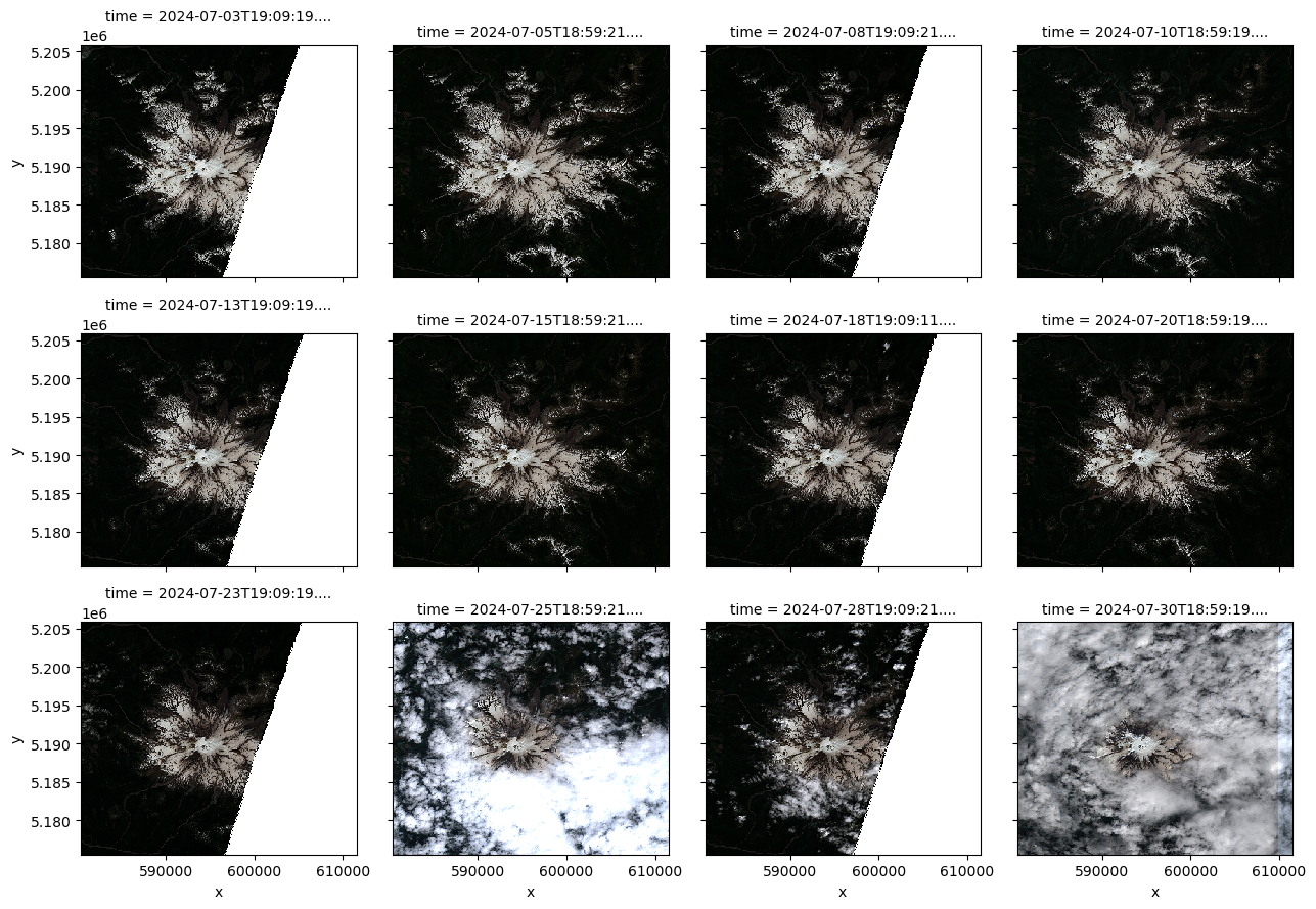
Plot a median RGB image for July 2024#
rgb_da.median(dim='time').plot.imshow(robust=True)
<matplotlib.image.AxesImage at 0x7efe4e3b46e0>
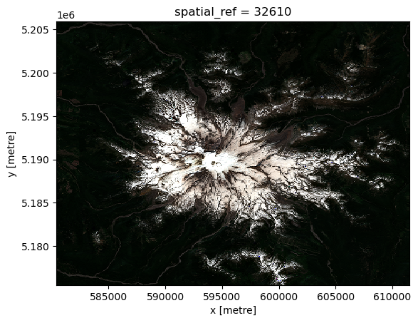
How can we tell when and where there are clouds?#
Check out the scene classification layer, SCL!
import matplotlib.colors
import matplotlib.ticker as mticker
# here's some colormap info
scl_class_info = {
0: {"name": "No Data (Missing data)", "color": "#000000"},
1: {"name": "Saturated or defective pixel", "color": "#ff0000"},
2: {
"name": "Topographic casted shadows",
"color": "#2f2f2f",
}, # (called 'Dark features/Shadows' for data before 2022-01-25)
3: {"name": "Cloud shadows", "color": "#643200"},
4: {"name": "Vegetation", "color": "#00a000"},
5: {"name": "Not-vegetated", "color": "#ffe65a"},
6: {"name": "Water", "color": "#0000ff"},
7: {"name": "Unclassified", "color": "#808080"},
8: {"name": "Cloud medium probability", "color": "#c0c0c0"},
9: {"name": "Cloud high probability", "color": "#ffffff"},
10: {"name": "Thin cirrus", "color": "#64c8ff"},
11: {"name": "Snow or ice", "color": "#ff96ff"},
}
scl_cmap = plt.cm.colors.ListedColormap([info["color"] for info in scl_class_info.values()])
class_values = sorted(list(scl_class_info.keys()))
bounds = [(class_values[i] + class_values[i + 1]) / 2 for i in range(len(class_values) - 1)]
bounds = [class_values[0] - 0.5] + bounds + [class_values[-1] + 0.5]
norm = matplotlib.colors.BoundaryNorm(bounds, scl_cmap.N)
ticklabels = [item['name'] for item in scl_class_info.values()]
s2_ds['SCL'].plot.imshow(col='time',
col_wrap=4,
cmap=scl_cmap,
cbar_kwargs={"ticks": class_values, "format":mticker.FixedFormatter(ticklabels)},
norm=norm,
robust=True)
<xarray.plot.facetgrid.FacetGrid at 0x7efe4eef5400>
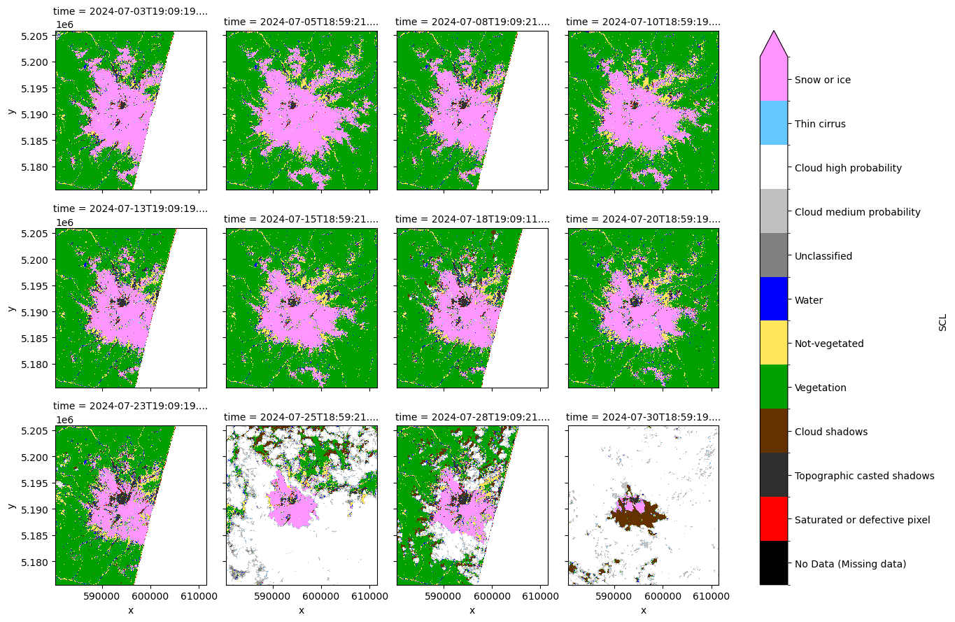
Calculate and plot an NDVI time-series#
ndvi_da = (s2_ds["B08"] - s2_ds["B04"]) / (s2_ds["B08"] + s2_ds["B04"])
ndvi_da
<xarray.DataArray (time: 12, y: 380, x: 389)> Size: 7MB
dask.array<truediv, shape=(12, 380, 389), dtype=float32, chunksize=(1, 380, 389), chunktype=numpy.ndarray>
Coordinates:
* y (y) float64 3kB 5.206e+06 5.206e+06 ... 5.176e+06 5.176e+06
* x (x) float64 3kB 5.804e+05 5.805e+05 ... 6.114e+05 6.115e+05
spatial_ref int32 4B 32610
* time (time) datetime64[ns] 96B 2024-07-03T19:09:19.024000 ... 202...ndvi_da.plot.imshow(col='time',col_wrap=4,robust=True,cmap='RdYlGn',vmin=-1,vmax=1)
<xarray.plot.facetgrid.FacetGrid at 0x7efe4ef76060>
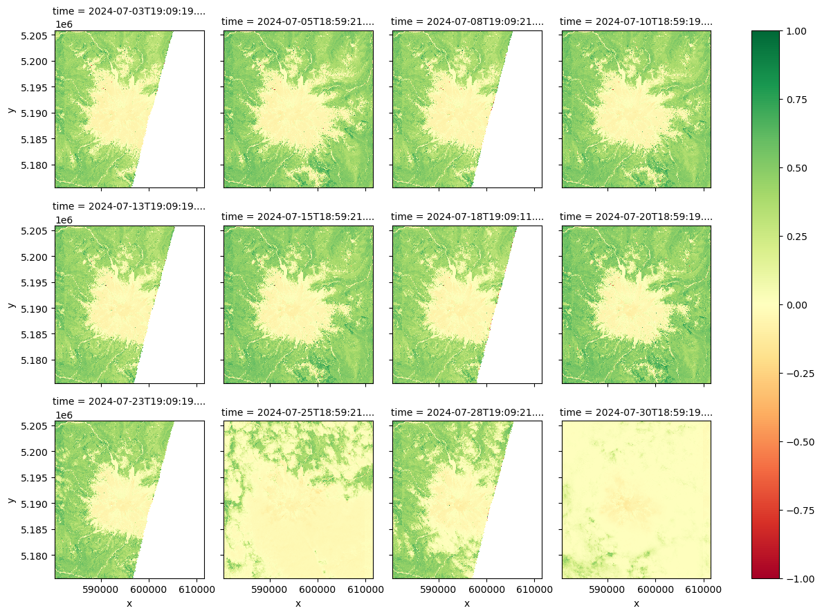
Try again, masking out bad data according to the SCL#
bad_scl = [0,1,2,3,8,9,10]
ndvi_masked_da = ndvi_da.where(~s2_ds['SCL'].isin(bad_scl)).compute() # What do you think compute does here?
ndvi_masked_da.plot.imshow(col='time',col_wrap=4,robust=True,cmap='RdYlGn',vmin=-1,vmax=1)
<xarray.plot.facetgrid.FacetGrid at 0x7efe4f292f00>
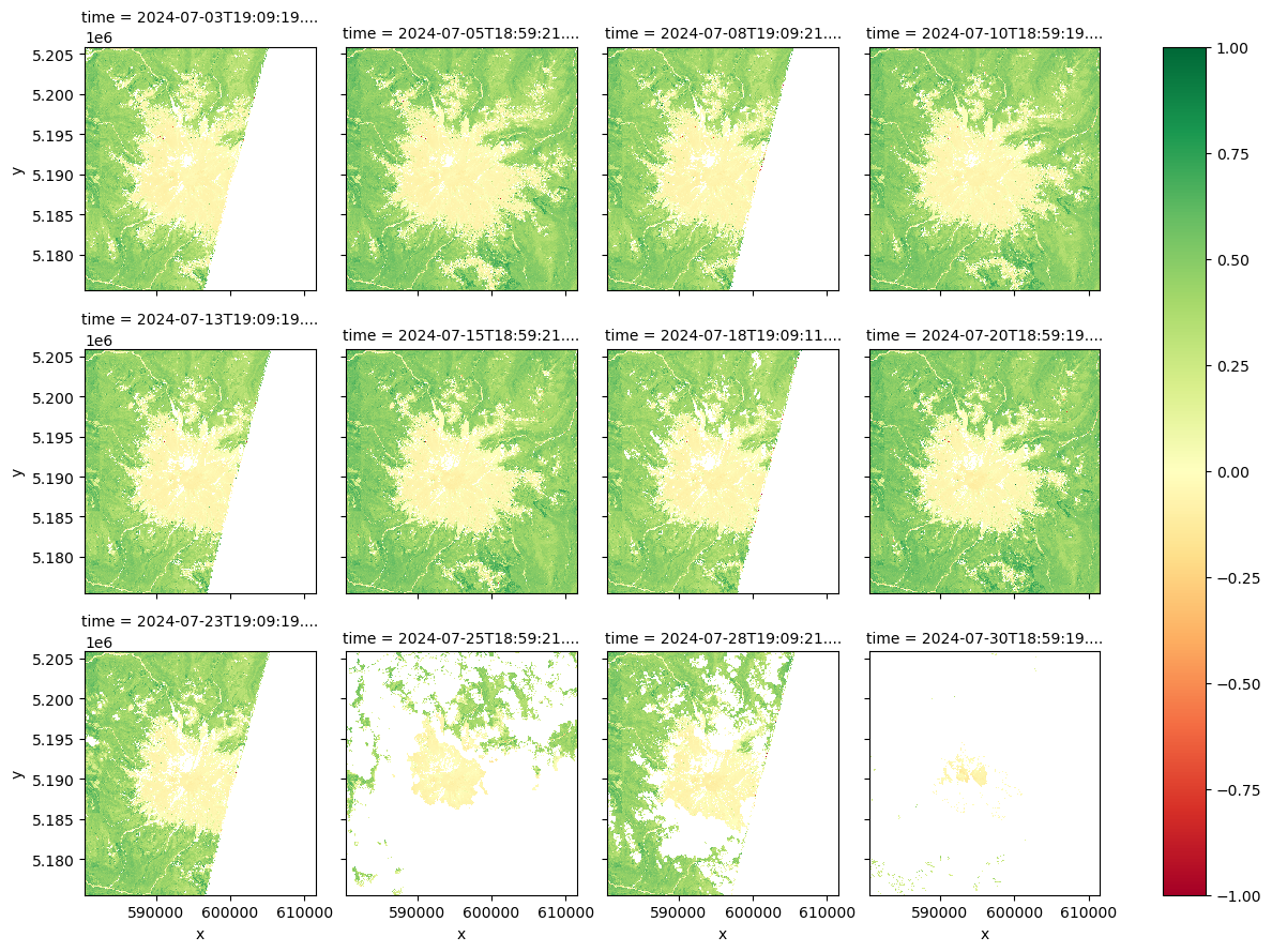
Plot a median NDVI image for July 2024#
ndvi_masked_da.median(dim='time').plot.imshow(robust=True,cmap='RdYlGn',vmin=-1,vmax=1)
<matplotlib.image.AxesImage at 0x7efe4d42c3e0>
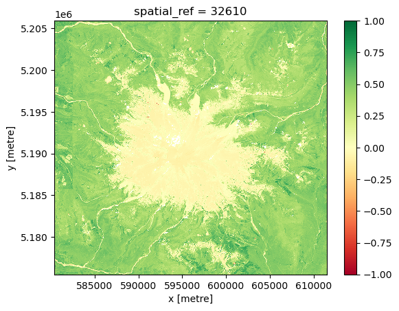
Create a median NDVI time-series#
# def not the best way to do this, but quick approximation
proportion_pixels_valid = ndvi_masked_da.count(dim=['x','y'])/ndvi_masked_da.count(dim=['x','y']).max()
proportion_pixels_valid
<xarray.DataArray (time: 12)> Size: 96B
array([0.63730512, 0.99736894, 0.65268564, 1. , 0.6497117 ,
0.99948918, 0.6696616 , 0.99463991, 0.63063649, 0.20557282,
0.48157556, 0.01757774])
Coordinates:
spatial_ref int32 4B 32610
* time (time) datetime64[ns] 96B 2024-07-03T19:09:19.024000 ... 202...f,ax=plt.subplots()
ndvi_masked_da.where(proportion_pixels_valid > 0.8).median(dim=['x','y']).plot.scatter(ax=ax,x='time',y='data')
ax.set_title('Median NDVI over time for images with >80% valid data')
ax.set_ylabel('NDVI')
ax.set_xlabel('Date')
ax.grid(True)